側向電場用於電泳顯示器之應用與特性探討

國 立 交 通 大 學

光電系統研究所

碩 士 論 文

側向電場用於電泳顯示器之應用與特性探討

Using Lateral Electric Field in Electrophoretic Displays for

Mechanism Understanding and Applications

研 究 生：許博鈞

指導教授：黃乙白 博士

鄭協昌 博士

中 華 民 國 一百零一 年 七 月

側向電場用於電泳顯示器之應用與特性探討

Using Lateral Electric Field in Electrophoretic Displays for

Mechanism Understanding and Applications

研 究 生：許博鈞 Student：Po-Chun Hsu

指導教授：黃乙白 Advisor：Yi-Pai Huang

鄭協昌 Advisor：Shie-Chang Jeng

國立交通大學

光電系統研究所

碩士論文

A Thesis

Submitted to Institute of Photonic System College of Photonics

National Chiao Tung University in partial Fulfillment of the Requirements

for the Degree of Master

in

Photonic System

July 2012

Hsinchu, Taiwan, Republic of China

側向電場用於電泳顯示器之應用與特性探討

碩士研究生： 許博鈞

1

指導教授： 黃乙白

2

副教授 與 鄭協昌

3

助理教授

國立交通大學 1 光電系統研究所 2 顯示科技研究所 以及3 影像與生醫光電研究所

摘要

利用 In-Plane 電極製造橫向電場，與使用顯微鏡以微觀的觀測方式量測電泳式顯 示器中微米粒子的運動情形，並運用 MATLAB 進行影像處理，以取出實驗所需的三種重 要參數(飄移速度、粒子排列對比以及擴散速度)用以比較各種基礎波型的特性，進而 得到粒子運動時的受力情形，並推導出運動時的受力模型，最後則可運用此特性改善 電泳式顯示器之反應速度、雙穩態以及對比度。另外在橫向的觀測中，亦可與一般縱 向的驅動作出關聯。 除此之外，亦可利用橫向電場進行電泳式顯示器的驅動，使用橫向電場進行重置， 則可於近乎無閃爍的狀態之下將正負離子中和進而得到更佳的雙穩態，並運用橫向電 場，先行布置粒子位置而得到更快的反應時間。此外，可以以單通道或雙通道的訊號 進行更高精細度的灰階調控，用以實現高灰階數以及降低殘影的成果。 當然，由於在此種基板設計下，雙穩態與殘影的問題即可大大縮小。若可將流體 更換為較低粘滯係數之材料，另可以得到更快的反應時間亦不會使得整個電泳式顯示 器的顯示品質降低太多。所以，未來可以由材料、驅動波形以及電極的形狀進行搭配 並優化，以得到高品質之電子紙。

Using Lateral Electric Field in Electrophoretic Displays for

Mechanism Understanding and Applications

Student: Po-Chun Hsu

1

Advisor: Yi-Pai Huang

2

and Shie-Chang Jeng

3

1

_{Institute of Photonic System, College of Photonics}

2

_{Display Institute, College of Electrical and Computer Engineering}

3

_{Institute of Imaging and Biomedical Photonics, College of Photonics}

National Chiao Tung University

Abstract

We proposed a lateral observation method for mechanism understanding. The lateral observation method could observe the particle position and measure the parameters of driving characteristics such as drifting speed, particle packing, and bistability lost. In lateral direction, there was no information shielding by the other particles which were closer to the light source in vertical observation. The slow response time, non-perfect bistability, and improvable extreme state were issues in electrophoretic display system. We could find out how the internal electric force affected those issues and make a solution.

On the other hand, the lateral driving method provided us another way to switch images. Using lateral reset could be a non-flicker reset for comfortable reading and enhance the transition time by separation the particles. Furthermore, dual side driving could build up a total different electric field in the same electrode for applications. Single side driving could fine tune the lightness by the curved and weak electric field. Double side driving could coarse tune the lightness in a short time. The number of gray levels and short term bistability could be increased.

Acknowledgements

首先，要誠摯的感謝實驗室兩位老師，謝漢萍教授和指導老師黃乙白副教授在碩 士兩年的求學生涯中提供豐富的實驗室資源和良好的研究環境。對於研究過程、研討 會報告與英文能力的指導鞭策，培養我進入社會後所應具備的基本條件。也由衷感謝 各位口試委員對於本論文所提供的寶貴建議，使整體內容更加趨於完備。 此外，更感謝林芳正助理研究員，在碩士生涯的指導與帶領，無論是對於論文研 究方向上的建議、在研究過程中遇到問題時的指導與幫忙、研討會報告與論文的修改， 還有精神上的鼓勵與打氣等，同時身為 FSC 與電子紙組別的支柱實在是非常辛苦。學 長除了具備超群的文書處理能力、表達能力，對於研究的熱誠與專業是讓我最佩服之 處，也成為我的學習榜樣。除此之外也謝謝同組已畢業的學姊吳思頤與同學楊上翰在 研究上的合作與幫忙，與你們一起實驗與問題討論是很振奮人心的事情。也謝謝合作 計畫公司的同仁楊柏儒、張明仁、黃若城學長，對於研究與實驗方向上面的建議、協 助與配合，使得一切能夠順利流暢的進行。 感謝實驗室台翔、精益、國振、凌堯、柏全、奕智、小皮、大頭、致維哥、與志 明等博班學長姐，提供各方面專業的指導與意見。也特別感謝上一屆學長姐小馬、小 頭、立偉、馬志堯、董哥、蓋 B、昌毅、小 fighter、博六、子寬和江濟宇等人，在我 碩一時的照顧。此外也謝謝碩二的同學張綺、拉拉、博凱、白諭、周秉彥、光電王子 王柏皓、冏務以及師父，在這兩年中無論是在研究、課業和生活上一起打拼與互相扶 持，讓實驗室增添許多趣味。另外，也要向實驗室的雅惠、穎佳、茉莉、江介堯和蓮 芳五位助理們還有學弟妹們表達最誠摯的感謝，讓我們在研究之餘無後顧之憂，並使 實驗室整體像一個大家庭一樣隨時充滿歡愉的氣氛。最後，對於我的家人及朋友們， 感謝你們這兩年來背後的關懷、鼓勵與陪伴，使我能夠無後顧之憂且順利地完成兩年 的碩士學位，這份感激與喜悅要分享給所有認識和幫助過我的人。

Table of Contents

摘要 ... iii Abstract ... iv Acknowledgements ... v Chapter 1. Introduction ... 1 1.1 Classification of E-papers ... 2

1.1.1 The Transmissive Type E-paper ... 2

1.1.2 Organic Light Emitting Diode ... 3

1.1.3 Mirasol Display ... 4

1.1.4 LC E-paper ... 5

1.1.5 Electrophoretic Display ... 6

1.2 The Types of Electrophoretic Displays ... 8

1.2.1 Microcapsule Electrophoretic Display ... 8

1.2.2 Quick Response Liquid Powder Display ... 9

1.2.3 Microcup Electrophoretic Display... 10

1.3 Motivation and Objectives... 11

1.4 Prior Arts of Lateral Electrode Design ... 12

1.5 Thesis Organization ... 13

Chapter 2. Mechanism ... 15

2.1 The Phenomena of Electrophoresis ... 15

2.1.1 The Formation of Charged Particle ... 15

2.1.2 The Electric Double Layer and Zeta Potential ... 16

2.1.3 Electrostatic and DLVO Theorem ... 19

2.1.4 The Bistability State ... 21

2.2.1 Paging Time ... 22

2.2.2 The Remnant DC ... 23

Chapter 3. Equipment & Method ... 25

3.1 Equipments ... 25

3.1.1 Photo Diode ... 25

3.1.2 Photometer ... 26

3.1.3 Function Generator ... 27

3.1.4 Laser Scanning Confocal Microscope ... 28

3.2 Observation System ... 29

3.2.1 The Macroscopic System Setup ... 29

3.2.2 The Microscopic System Setup ... 29

3.3 Evaluation Indexes ... 31

3.3.1 Particle moving velocity v(t) ... 32

3.3.2 Particle Packing Contrast ... 32

3.3.3 Lateral Bistability (Repulsing speed) ... 33

Chapter 4. Simulations ... 34

4.1 Simulation Tool ... 34

4.2 Simulation for Electric Field Distribution ... 35

4.3 Simulation for Hydromechanics ... 37

4.4 Optimization for Real Product Case ... 38

Chapter 5. Experimental Results ... 42

5.1 Mechanism Confirmation ... 42

5.1.1 Experiment of Moving Velocity v(t) ... 43

5.1.5 Correlation with Lateral and Vertical ... 49

5.2 Application Proposition ... 51

5.2.1 Lateral Reset ... 52

5.2.2 Dual Side Driving Characteristic ... 54

5.3 Summary ... 62

Chapter 6. Conclusion and Future Work ... 64

6.1 Conclusion ... 64

Figure Captions

Fig. 1-1 E-paper products (a) E-books. (b) Flexible displays. (c) Price tags.

(d)Smart cards. ... 1

Fig. 1-2 The e-paper technologies including reflectivity and contrast ratio. ... 2

Fig. 1-3 The prior arts of e-paper technologies. ... 3

Fig. 1-4 The structure of the OLED. ... 4

Fig. 1-5 Mirasol display working principle. ... 4

Fig. 1-6 The principle for BiNem with different driving pulse. ... 5

Fig. 1-7 The principle for ChLC shows the image. ... 6

Fig. 1-8 EPD can be read under sunlight and LCD will see nothing. ... 7

Fig. 1-9 When switching pages the previous image still remaining. ... 7

Fig. 1-10 After several hours the bright region became darker and vice versa. ... 7

Fig. 1-11 The display method in microcapsule EPD. ... 9

Fig. 1-12 The QR-LPD structure. ... 9

Fig. 1-13 The microcup EPD structure. ... 10

Fig. 1-14 The operation principle of mircocup EPD. ... 11

Fig. 1-15 The comb-like electrode for the lateral electric field. ... 12

Fig. 1-16 The main lateral electric field functions. ... 13

Fig. 2-1 The diagram for phenomena of electrophoresis. ... 15

Fig. 2-2 The surfactant working function. ... 16

Fig. 2-3 Scheme of the ion distribution around the charged particle. The gray circle is the charge density around TiO2, the darker the denser. ... 18

Fig. 2-4 Potential variation with distance for a charged surface: (a) potential reversal due to adsorption of surface, (b) adsorption of surface. ... 19

Fig. 2-6 Schematic showing paging time effect. ... 22

Fig. 2-7 Schematic showing remnant DC effect. ... 23

Fig. 3-1 The photoelectric effect. ... 26

Fig. 3-2 The PDA100A photo diode. ... 26

Fig. 3-3 The Photometer, I-one. ... 27

Fig. 3-4 The Agilent 33210A function generator. ... 27

Fig. 3-5 The IX71 laser scanning confocal microscope. ... 28

Fig. 3-6 The light path in macroscopic system. ... 29

Fig. 3-7 The light path of the microscope system. ... 30

Fig. 3-8 The flow chart of MATLAB programming. ... 31

Fig. 3-9 (a) The top view of the video was picked up frame by frame in transmissive mode. (b) The white track was the particle motion in different time along X direction. ... 32

Fig. 3-10 The top view of the cell. Black and white area has high concentration of black and white particles respectively. Yellow area has few particles. ... 33

Fig. 4-1. The cross section of electric distribution in the cell, working ratio is defined as A working (red dashed square)/A (yellow solid square). ... 35

Fig. 4-2 (a) The conditions with L fixed at 100 um. (b) W fixed at 50 um. Red curves are electric field along the lateral direction. Blue ones are working ratio. ... 36

Fig. 4-3 The electric field distribution in W= 50 μm L= 200 μm lateral operation. 36 Fig. 4-4 The particle flow in W = 50 μm L = 200 μm lateral operation. ... 37

Fig. 4-5 The velocity strength in W = 50 μm L = 200 μm lateral operation. ... 38

Fig. 4-6 Normalized working ratio with acceptable electric field (Ex > 0.3 V/μm) 39 Fig. 4-7 The voltage distribution in W = 5 μm L = 20 μm lateral operation. ... 39

Fig. 4-9 The velocity distribution in W = 5 μm L = 20 μm lateral operation. ... 41

Fig. 4-10 The velocity field distribution in W = 5 μm L = 20 μm lateral operation. 41 Fig. 5-1 The basic waveforms are DC, shaking, and pulsing. ... 42

Fig. 5-2 The curves including different driving time and waveforms are plotted as the particles maximum speed. ... 43

Fig. 5-3 The particle packing contrast versus voltage curves are plotted containing different driving time and waveforms. ... 45

Fig. 5-4 (a) Short term bistability (b) long term bistability including different driving time and waveforms are plotted in versus voltage. ... 46

Fig. 5-5 The forces happened when diving. ... 48

Fig. 5-6 The screening field caused the repulsive electric field. ... 48

Fig. 5-7 The stable state force evolution. ... 49

Fig. 5-8 The optical responses in different voltage at vertical direction. ... 50

Fig. 5-9 The expected model forms the gray levels with white and black particle. (a) The optical response was not dominated by the concentration of the particles. (b) Different voltage packed the different purity of particles. ... 50

Fig. 5-10 The lateral driving method setup. ... 51

Fig. 5-11 The lateral reset waveform by the opposite polarity in signal 1 and 2. .... 52

Fig. 5-12 The lateral reset could prevent collision by separating the particles. ... 52

Fig. 5-13 The comparison of reset waveform. ... 53

Fig. 5-14 The particles moving in the lateral reset. ... 53

Fig. 5-15 Comparison of improved driving and vertical driving (a) Improved image transition including reset waveform (b) Vertical driving including reset. ... 54

Fig. 5-18 The electric field distribution in single side driving. ... 56

Fig. 5-19 The double side driving (a) waveform and (b) optical response. ... 56

Fig. 5-20 The electric field distribution in double side driving. ... 57

Fig. 5-21 The 30 volt double side driving (a) waveform and (b) optical response .. 58

Fig. 5-22 The double side driving (a) waveform with 15 and 30 volt pulsing after 30 volt DC and (b) optical response. ... 59

Fig. 5-23 The mixture waveform. ... 60

Fig. 5-24 Comparison of vertical driving and improved driving (a) Flicker and response time (b) Bistability ... 61

Fig. 6-1 The proposed waveform for quick response, high contrast ratio and stable lightness. ... 65

Fig. 6-2 The particles transition direction. ... 66

Fig. 6-3 The coarse adjustment. ... 66

Fig. 6-4 The fine adjustment. ... 67

List of Tables

Table 1-1 The prior arts of EPD. ... 8

Table 2-1 Magnitudes of the characteristic force when temperature is 300K, particle diameter is 1um, surface electric potential is 5V, velocity is 1um/s, density is 103 kg/m3 and viscosity is 10-3 Pa∙s. ... 21

Table 5-1 The comparison of conventional and In-Plane EPDs. ... 62

Table 6-1 The effects of W and L in the microcup EPD. ... 64

Chapter 1. Introduction

Nowadays, green technology becomes more and more popular. Especially, green display technology is one of the most popular technologies in the world. The electrophoretic display (EPD) [1] has been regarded as one of the dominant technologies of E-paper in the green display technology. It has several advantages such as wide viewing angle, operation without backlight, readability in sunlight ambience, flexibility and unbreakability. It can be not only low power consuming but also thinner and lighter.

Some companies have invested in the e-paper technology for years, such as AUO, Bridgestone, Qualcomm, Fujitsu, and Philips. They have put a lot of people and money to win the competition of e-paper. Therefore, many e-paper technologies were developed quickly and the products were manufactured for living needs as shown in Fig. 1-1

Fig. 1-1 E-paper products (a) E-books. (b) Flexible displays. (c) Price tags. (d)Smart cards.

(a)

(b)

(c)

(d)

http://www.cio360.net/Portals/0/ipad_2up_hom etimes.jpg http://www.geeky-gadgets.com/wp-content/ upl oads/2010/08/Flexi ble-ePaper1.j pg

1.1 Classification of E-papers

There are lots of E-paper technologies in the world as shown in Fig. 1-2. Generally, the technologies are divided into two kinds: lighting (transmissive or emissive) and reflective type. The lighting ones have the better image quality, and the other ones provide the comfortable reading experiment.

Fig. 1-2 The e-paper technologies including reflectivity and contrast ratio.

1.1.1

The Transmissive Type E-paper

The transmissive and emissive types function as liquid crystal displays (LCDs) or organic light emitting diodes (OLEDs) having 8-bit gray levels, higher contrast ratio, wide color rendering and fast response time which make them possible to play videos. However, the viewing angle of LCD is limited and this technology has color shift issue. Nevertheless,

makes people comfortable just like reading a paper, and has the benefit in power consumption. These superiorities make people able to read for a long time and it can replace the book in next generation. Therefore, the most popular technologies of the E-paper are Mirasol display, LC E-paper, and EPD as shown in Fig. 1-3.

Fig. 1-3 The prior arts of e-paper technologies.

1.1.2

Organic Light Emitting Diode

Organic light emitting diode (OLED) [2] is a device without viewing angle limitation and has high brightness because of self-emissive as shown in Fig. 1-4. It can be operated without backlight and ambient light. It lights when electron and hole are combined, so the response time is fast. However, OLED still has some disadvantages, such as short life time, high cost, difficulty to manufacture and unfavorable sunlight readability.

E-Paper OLED Organic Light-Emitting Diode Mirasol LCD

Liquid Crystal Display

Bistable Twisted-Nematic Cholesteric Liquid Crystal

EPD

Electro Phoretic Display

Micro Capsules Microcup

QR-LPD

Quick-Response Liquid Powder Display

Fig. 1-4 The structure of the OLED.

1.1.3

Mirasol Display

Mirasol display [3] was invented by Mark W. Miles, a MEMS researcher and founder of Etalon, Inc., and co-founder of Iridigm Display Corporation. The principle of Mirasol is using interference of light by micro electro mechanical system (MEMS) as shown in Fig. 1-5. It has fast response time, colorful image and low power consumption with bistability. By using the MEMS fabrication process, Mirasol display is very expensive.

1.1.4

LC E-paper

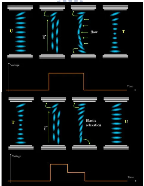
LC e-paper can be classified into two types: bistable LC and cholesterol LC (ChLC). In bistable LC type, BiNem [4] is a breakthrough technology that enhances existing LCD technologies by providing a memory effect and superior image quality. It is based on a unique principle called “surface anchoring breaking” fully patented by Nemoptic. BiNem technology has two stable states, the Uniform (U) state and the Twisted (T) state as shown in Fig. 1-6.

Fig. 1-6 The principle for BiNem with different driving pulse.

The other one is ChLC [5] which is a type of liquid crystal with a helical structure and it is therefore chiral. The operation principle is that lights are reflected in the planar texture to reveal the bright state, while lights transmit and are scattered in the focal conic texture and reveals dark state as shown in Fig. 1-7.

Fig. 1-7 The principle for ChLC shows the image.

1.1.5

Electrophoretic Display

EPDs usually show the image by manipulating the position of black and white charged particles [14]. The charged particles are prepared with the pigments mixing with the surfactants in the non-polar solvent [15]. Upon applying an external electric field, the charged particles move along the electric field and display images by mixing the different percentage of particles [16].

EPD is a thin, light, robust, and flexible display, and is readability under the sunlight ambience as shown in Fig. 1-8. According to its bistability [6] characteristic, EPD requires a voltage only when switching the images. With this phenomenon, EPD is totally different from an e-paper using conventional LCDs and OLEDs. However, EPD still has some issues such as slow response time, flicking effect when changing the pages, ghost images as shown

Fig. 1-8 EPD can be read under sunlight and LCD will see nothing.

Fig. 1-9 When switching pages the previous image still remaining.

Fig. 1-10 After several hours the bright region became darker and vice versa.

display. Moreover, EPDs’ reflectivity is the highest one in the E-paper products. On the other hand, as a reader, EPD has zero power consumption when the image was not changing because of the bistability. It only consumes the electricity when image switches.

1.2 The Types of Electrophoretic Displays

The electrophoretic display (EPD) is regarded as one of the dominant technologies of E-papers in green display technologies. There are three main EPD skills in Table 1-1.

Table 1-1 The prior arts of EPD.

1.2.1

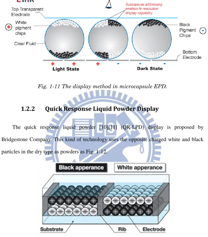
Microcapsule Electrophoretic Display

The microcapsule EPD [7]-[9] is invented in MIT and produced by E-ink Company. It has microcapsules which load the black and white opposite charged particles to form the different reflectivity as shown in Fig. 1-11. When the bottom electrode was exerting positive voltage, the negative particles would swim to the bottom, vice versa.

Microcapsule EPD Microcup EPD QR-LPD

Driving Method

Reflectivity 50％ 40％ 40%

Transition Time ~300ms ~300ms 0.2ms

Driving Voltage ±15V ±15V ~70V

Driving AM/PM AM/PM PM

Contrast Ratio 10:1 10:1 10:1

Color by color filter by color solvent by color filter

Fig. 1-11 The display method in microcapsule EPD.

1.2.2

Quick Response Liquid Powder Display

The quick response liquid powder [10][11] (QR-LPD) display is proposed by Bridgestone Company. This kind of technology uses the opposite charged white and black particles in the dry type as powders as Fig. 1-12.

Fig. 1-12 The QR-LPD structure.

When applying voltage, the corresponding particles would flow downstream or upstream just like the microcapsule EPD. But the driving condition is totally different from the microcapsule EPD by the solid state powder and using air as a solution. By doing so, the

transition time is much faster than the other EPDs, but the driving voltage is too high to build on the active matrix.

1.2.3

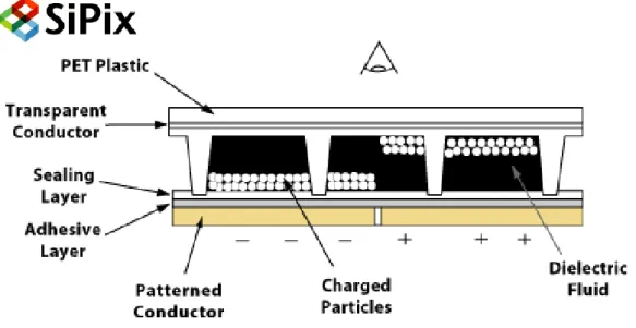
Microcup Electrophoretic Display

The microcup EPD [12] is provided by SiPix Company. It is made up of matrix of cups typically 150 μm in width. The whole display has strong strengths because of the microcup structure which is more applicable in flexible displays and which fits into roll to roll manufacture. It can be made square or hexagon as shown in Fig. 1-13.

Fig. 1-13 The microcup EPD structure.

When bottom electrode was exerting negative voltage, the positive charged particles would swim to the bottom and the other side shows the fluid in black. In other words, when bottom electrode was exerting positive voltage, the charged particle would swim along the electric field to the top of the microcup, and shows white as shown in Fig. 1-14.

Fig. 1-14 The operation principle of mircocup EPD.

Although the transition time of a microcup EPD is not fast enough compared to the QRLPD, the microcup EPD has lower manufacturing cost due to roll-to-roll process [13] and color can be realized by color solvent instead of inefficient color filters, which increases the overall whiteness. Therefore, the microcup EPD was chosen to be our research objective.

1.3 Motivation and Objectives

Since 1979, M. A. Hopper and V. Novotny proposed the EPD model by optical simulation and experiment, the model was modified several times in a half hundred years. In those models, the optical response was observed in such different ways to confirm the correctness of their model [16]-[19]. However, the electrophoresis happens in a micro meter scale, the macroscopic observation has less persuasiveness. Therefore, we want to use the microscopic observations to fully understand the mechanism in the electrophoretic display and develop the new application with lateral electric field in the microcup EPD by the comb-like electrode as shown in Fig. 1-15.

Fig. 1-15 The comb-like electrode for the lateral electric field.

On the other hands, EPD technology face difficult issues such as slow response time, ghost image, non-perfect bistability, paging time issue, and the flicking effect when switching the pages. We want to use both lateral and vertical electric field for more degree of freedom driving method to solve those issues. Flicker should be eliminated (∆L*< 1) for comfortable reading, response time should be shorter than 500 ms for human patience in nowadays and short term bistability lost should be lower than ∆L* < 1 due to the human awareness. Because the trend of the green display is irresistible, this job is important and needed. We have had to solve those issues and formed the hopeful future.

1.4 Prior Arts of Lateral Electrode Design

The lateral electrode design is developed to switch the reflectivity by the shielding percentage in Philips Company and Canon Company or the mixture percentage in SiPix Company as shown in Fig. 1-16.

Canon used the mirror-like reflective substrate to form the white state, and put the black particle to shield the substrate to form the dark state [20]-[22]. The lateral electric field was used for driving the particles in or out the reflective region and to show the image.

Philips made the shielding region to hide the reflective particles to form the dark state.

EPD Film

ITO Electrode

Signal #1

ITO Electrode

Signal #2

switch the images, so that Philips used the lateral electrodes [23][24].

Also, SiPix Company proposed the electrophoretic display with dual mode switching [25][26]. Dual mode switching comprised the vertical and lateral directional electric field to form the more freedom driving method. This method not only prevented the undesired movement of the charged particles in the cell but also provided the high image quality. Moreover, with dual mode switching, the color EPD would be developed without color filter.

Philips and Canon used lateral electric field to form the image just because their image formation method was dominant by the area in X-Y plane. SiPix used lateral electric field to form the color image. They did not eliminate the flicking effect or internal electric field for the bistability and transition time.

Fig. 1-16 The main lateral electric field functions.

1.5 Thesis Organization

The thesis is organized as follows: the fundamental properties, the charge and bistability mechanisms of a microcup EPD are introduced in Chapter 2. Besides, the

instruments used in the experiment and the measurement skills are described in Chapter 3. The simulation results of the electric field distribution for the electrode design are in Chapter 4, and experimental results and new driving method are discussed in Chapter 5. Finally, conclusion, minor issues and the future work are presented in Chapter 6.

Chapter 2. Mechanism

2.1 The Phenomena of Electrophoresis

There are four main types of electrokinetic in the fluid: electroosmosis, streaming potential, electrophoresis, and sedimentation potential [6]. Electrophoresis describes the motion of dispersed particles relative to the fluid under the influence of spatially uniform electric field. The dispersed particles with surface charge cause the Coulomb force by external electric field. This phenomenon was found in A.D. 1807 by Reuss, who do the experiments for constant electric field causing the clay particles in water to migrate as Fig. 2-1. After that, electrophoresis researches have been one of the important parts of the colloid and surface science.

Fig. 2-1 The diagram for phenomena of electrophoresis.

2.1.1

The Formation of Charged Particle

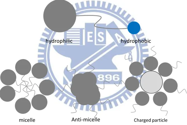
Making the charged particles was the first thing to make the electrophoretic environment. As t he total charge was zero, the surfactant which has hydrophilic and hydrophobic ends was needed for charging the particles and solvent. Surfactant dissociates

and adsorbs on the different pigment to form the charged particles [27]. And some dissociated surfactant aggregates together forming the micelles [28] or anti-micelles as shown in Fig. 2-2.

The electric field could affect the particles with charge. On the other hands, the micelles and anti-micelles would be affected by the electric field too. Only the colored particle formed the image, yet the quantities of micelles and anti-micelles would influence the image quality because the micelles, anti-micelles and dissociated surfactant moves first, which make the internal electric field to stop the charged particles.

Fig. 2-2 The surfactant working function.

2.1.2

The Electric Double Layer and Zeta Potential

Colloid science [6] usually uses the electric double layer and zeta potential for describing the attractive or repulsive force. According to the Boltzmann distribution, the

hydrophilic

hydrophobic

and T is temperature. For example, the black positive charged particle carried negative charged ion with high concentration outside formed a negative potential layer, called Stern layer. Then, the negative charged ions attached to the colloid continuously but blended some positive ions. This second layer is loosely associated with the object, because it is made of free ions which move in the fluid under the influence of electric attraction and thermal motion rather than being firmly anchored. It is thus called the diffuse layer.

B ze k T

e

 



(1)

When the spherical surface is considered, Poisson-Boltzmann equation is used to solve the problem. The formula was written as shown in Eq.(2), where r is distant, ψ is potential, z is valency, e is electron charge, n is ionic concentration, ε is permittivity, k is Boltzmann constant, and T is temperature. In this formula, there is no analytical solution, so Debye-Huckel approximation is needed.

With Debye-Huckel approximation,

1 2 2 2 2 ( ) B e z n k T





 and B ze k T



  were defined. Also,

r

a

(1

X

)

a







was substituted for thin double layer where



a

1

_{was assumed,} and κ -1 meant the covered ions distance called Debye length. The formula can be rewritten as shown in Eq.(3), and the solution of energy distribution can be solved as shown in Eq.(4).

2 2

1

2

(

)

sinh(

)

B

d

d

ezn

ze

r

r dr

dr

k T









₍₂₎ 2 2

2

sinh

(1

)

d

d

X

dX

dX

a

a

















(3) ( ) 0 r a

a

e

r

  

  

₍₄₎

Fig. 2-3 Scheme of the ion distribution around the charged particle. The gray circle is the charge density around TiO2, the darker the denser.

In real case, ions are of finite size and they can approach a surface to a distance not less than their radius. Ions form the diffuse mobile part of the electric double layer whose centers are located beyond the Stern plane. There is a surface which is located between one to two radii away from Stern plane referred to as the shear plane as shown in Fig. 2-3. The shear plane referred to the electrokinetic potential, called zeta potential. The zeta potential is

Shear plane

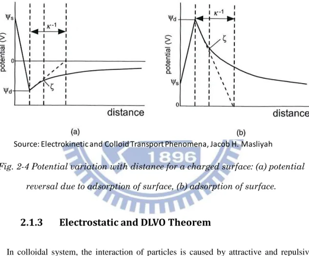
It should be noted that adsorbed ions can have marked effects on the zeta potential when compared with the surface potential. The counterions can cause reversal of charge within the Stern layer as shown in Fig. 2-4, where ζ is zeta potential and κ -1 is Debye length. Therefore, the zeta potential does not give direct information about the surface potential when adsorbed ions are presented. As the zeta potential, the interaction due to the mobility would happen no matter when external or internal electric field was induced.

Fig. 2-4 Potential variation with distance for a charged surface: (a) potential reversal due to adsorption of surface, (b) adsorption of surface.

2.1.3

Electrostatic and DLVO Theorem

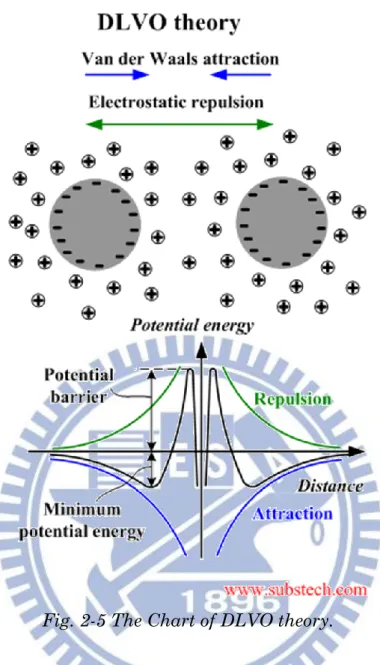
In colloidal system, the interaction of particles is caused by attractive and repulsive forces. For systems, the electrostatic and van der Waal force are dominant in the stable environment. Therefore, if the system is in a stable state, the force should be balanced with electrostatic repulsion due to the electric double layer and dispersion attractive force by London-van der Waals force. The concept was proposed by Derjaguin, Landau, Verwey, and Overbeek at A.D. 1941 to A.D. 1948. It is called DLVO theory as shown in Fig. 2-5.

Fig. 2-5 The Chart of DLVO theory.

As electromagnetic theorem, applying the external electric field would cause the electric force described as F QE_ex. And according to the Gaussian’s law, the charge was calculated as shown in Eq.(5), where ζ is zeta potential and Eex is external electric field.

Therefore, the force with external electric field was solved as shown in Eq.(6).





2 2 2

1

1

4

[

]

4

a

a

d

d

Q

r

r

dr

a

r dr

dr

a













 





_

_









(5)

4

_ex

(1

)

F



 

a

E





a

(6)

2.1.4

The Bistability State

The bistability state was a more important factor for the EPD than the LCD. With bistability, image would not change without signals. It gives the comfortable reading experience and low power consumption.

Here is the way to keep the image stable: stop the particles by force balance as Section 2.1. With the balance force, the pigments would not move heavily, so that the image could be the same. There are several forces in the electrophoretic system: external electric force, internal electric force, viscosity, surface tension, gravitational force, buoyancy, van der Waal force between each particle, and Brownian’s motion. The magnitude order of each force is shown in Table 2-1, the electrical force is the most important of all when driving and holding the image [29]. Therefore, how to adjust electric field is an essential art.

Table 2-1 Magnitudes of the characteristic force when temperature is 300K, particle diameter is 1um, surface electric potential is 5V, velocity is 1um/s,

density is 103 _kg/m3 _{and viscosity is 10}-3 _Pa∙s.

Force type

Force order

Electrical force

Brownian force

10

5

Attractive force

Brownian force

1

Viscous force

Brownian force

1

Gravitational force

Brownian force

10

-1

Internal force

Brownian force

10

-6

2.2 The Non-perfect Image Effect

There are some effects leading to the lower image quality, such as paging time and remnant direct current (RDC). These two effects cause the particles moving to the wrong place and showing the wrong reflectivity. The main reason is the different internal force and initial position. If every time EPD is driven in the dissimilar environments, the reflectivity would not be the same with typical driving waveforms.

2.2.1

Paging Time

When we read a book, the image stays constant for a long time, and the time interval of switching each pages is called paging time. Paging time could be regarded as the stage for ion recombination. When voltage offs, the particle should keep the original position. However the internal electric field would force particles and ions to the lowest potential state, so the movement happens [30]. Consequently, the next time when we switch the pages, the internal force and position of the particles are not the same as shown in Fig. 2-6, depending on the paging time. And this effect affects the image quality greatly.

Due to this effect, the driving waveform usually does a reset process for a same initial state. With the reset process, the image could be displayed the same after different paging time. However, the reset process takes a lot of time and sometimes follows the flicking effect which causes people uncomfortable. Therefore, how to eliminate the paging time effect or optimize the reset process has been an important job in this research field.

2.2.2

The Remnant DC

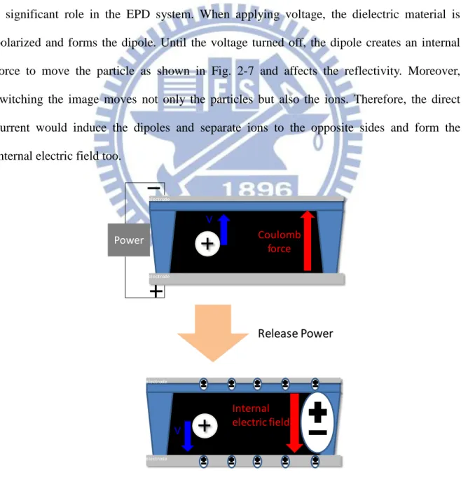
According to the importance of the internal field, the remnant direct current must play a significant role in the EPD system. When applying voltage, the dielectric material is polarized and forms the dipole. Until the voltage turned off, the dipole creates an internal force to move the particle as shown in Fig. 2-7 and affects the reflectivity. Moreover, switching the image moves not only the particles but also the ions. Therefore, the direct current would induce the dipoles and separate ions to the opposite sides and form the internal electric field too.

Fig. 2-7 Schematic showing remnant DC effect.

electrode electrode Coulomb force Power V electrode electrode V Internal electric field Release Power

Because of this effect, the driving waveform must add some alternating current pulse to combine the ions or relax the dipoles. For the better quality, the DC balance waveform must be needed to further reduce the remnant DC. Nevertheless, the driving waveform would become longer. Therefore, the lateral driving method might be the solution without remnant DC in shorter waveforms.

Chapter 3. Equipment & Method

In the EPDs measurement, the optical response is the most intuitional for the image quality. Moreover, the microscopic transportation phenomenon is also the thing that we want to understand. So, some equipment and method were needed to get that information.

Photo detection system and microscope system were needed for all optical response not only macroscopic but also microscopic observations. The microscopic lateral observation was needed to get information of particle moving speed, particle packing contrast, and stability in the cell for the transportation phenomenon.

3.1 Equipments

3.1.1

Photo Diode

The optical response was measured by photo diode which worked by photoelectric reaction. Einstein explained the photoelectric effect in A.D. 1887, which occurred because photons collided with electrons and brought up current. The formula was described as shown in Eq.(7), where h is Plunk constant, ν is frequency, ϕ is work function of the material, e is electron charge, and V is voltage of the electron.

It meant that when high energy photon stroke material, the electron in the material would be dissociated with potential eV and absorbed the photon one-on-one as shown in Fig. 3-1. Therefore, in the suitable frequency, the higher reflectivity caused the higher current. In our case, the photo diode which is manufactured by THORLABS Inc. with model number of PDA100A was used for visible light as shown in Fig. 3-2. This photo diode’s active areas has 9.8 mm diameter for enough signal in the Lambertian reflectance and also the detection wavelength is 350 to 1100 nm including visible light.

h

 

 

eV

(7)

Fig. 3-1 The photoelectric effect.

Fig. 3-2 The PDA100A photo diode.

3.1.2

Photometer

To prevent the drawback of the photo diode, only the relative signal it showed, the photometer was needed for the luminance information. I-one was chosen for the CIE-Lab measurement and purchased from HomDa Automation Co., Ltd. shown in Fig. 3-3. I-one has the 3.5 mm2 active area and 200 Hz scan rate for the experiments, and it can measure

Fig. 3-3 The Photometer, I-one.

3.1.3

Function Generator

During the experiments, the waveform which drove the film was generated by the function generator. The Agilent 33210A with option 001 as shown in Fig. 3-4 was used for the synchronized waveform to each electrodes and the common electrode. The way to synchronize two function generators was connecting them to the time base. If two function generators were connected, the master time base could be the time base output from one of the generator.

Fig. 3-4 The Agilent 33210A function generator. http://www.getop.com/upload_image/ news_news/ 59/X-Rite% 20i1%20Pro.j pg

This function generator can build up the arbitrary waveform which the experiments needed. Putting waveforms into the EPD film, the characteristics were shown and the quality of EPD would be further improved.

3.1.4

Laser Scanning Confocal Microscope

In microscopic observation, microscope was needed. The Olympus IX71 laser scanning fluorescent confocal microscope as shown in Fig. 3-5 was used for the microscopic optical and particle movement understanding.

Fig. 3-5 The IX71 laser scanning confocal microscope.

It contents transmissive mode, reflective mode, and laser scanning mode. Transmissive mode was used for the interval of the particles detection; the interval of the particles was distinguished by the light source of haloids lamp forming the higher color saturation.

scanning mode operated laser to be light source for the much higher resolution and the function of confocal showed the focal plane image only. All of the modes resolution were higher than 1 um for the electrophoretic particles.

3.2 Observation System

3.2.1

The Macroscopic System Setup

The 5mW and 632.8 nm wavelength He-Ne laser was set to be the light source and reflected by EPD film. The relative optical response was measured by photo diode as shown in Fig. 3-6, and the absolute lightness value was measured by photometer: I-one [31].

When the different waveforms were put into the EPD film, the instantaneous optical response and the stability of the reflectivity were measured. It was helpful to fine tune the waveform and find out the inadequate part.

Fig. 3-6 The light path in macroscopic system.

3.2.2

The Microscopic System Setup

Moreover, microscopic system was operated for tiny disparity which was hard to be seen. The microscopic system, including two modes of reflective and transmissive, was set

Photo-diode

He-Ne LASER

Microcup EPD film

Lambertian reflectance

up to observe the motion of particles inside an EPD, as shown in Fig. 3-7. The optical microscope was operated in the reflective mode to distinguish the luminance states of gray level 0 and gray level 15, respectively.

The optical transmissive mode was used for distinguishing the low concentration part of white and black particles which meant only few particles there. The images were captured instantaneously by a digital video camcorder. Then, three important indexes,

including particle moving speed, particle packing contrast, and lateral bistability were introduced to the efficiency of lateral electric field intensity and the stability of the particles. The driving quality was evaluated by these three parameters, and what happened to waveforms in the experiments was found out.

Hg

Lamp

Transflective

cube

Objective

Haloids

Lamp

EPD film

Digital

Camera

Image

Processing

The digital image processing used HSL (Hue, Saturation, and Lightness) color space to build the different regions which were white particles, black particles, and few particles in MATLAB programming calculations. The algorithm was shown as shown in Fig. 3-8.The region without particles was deselected by higher saturation light because the haloids lamp light would transmit directly. The gray levels were distinguished by the light intensity. Therefore, the particles distribution could be recognized and analyzed.

Fig. 3-8 The flow chart of MATLAB programming.

3.3 Evaluation Indexes

There were three parameters for analyzing the experimental results. These parameters were: moving velocity, particle packing contrast, and lateral bistability. These three parameters could be compared to obtain those basic test waveforms’ driving advantages, and then we combined those advantages by adding the basic waveform in the driving waveform at the suitable position. The objective was to design the fast response and high contrast ratio driving waveform in the normal direction by observing the phenomena in lateral direction. It might improve the performance logically and physically.

Digital Video

Digital Image _{every frame}

Image only with particles

De-high saturation

White Particles

Black Particles

Lightness Judgment

Integrate Panel Brightness X-t Image every

row

Image

3.3.1

Particle moving velocity v(t)

Particle moving speed, v(t), was proportional to the electric field in lateral direction. v(t) was utilized to estimate whether the electrode design had enough electric field along the lateral direction. Particle position of time, x(t), was acquired by analyzing from the video recorder. Deriving x(t), v(t) was got to determine the magnitude of the lateral electric field, as shown in Fig. 3-9.

(a) (b)

Fig. 3-9 (a) The top view of the video was picked up frame by frame in transmissive mode. (b) The white track was the particle motion in different time

along X direction.

3.3.2

Particle Packing Contrast

Particle packing contrast meant that particles were pushed together by a lateral electric field. The stronger the effective lateral electric field was, the more intensive the particle position was. We used image processing to get this parameter as shown in Fig. 3-10(a).

It had low concentration in area A, and high concentration in B. Summing these two area and dividing A by B meant the lateral electric field efficiency to drive those particles in Eq.(8), where AA and AB denotes the space at a point in area A and B respectively . When

Frame=1 x Frame =320 Frame=1 x Frame =320 4 5 6 7 8 9

i j A i B j

A

Particle Packing Contrast

A







(8)

3.3.3

Lateral Bistability (Repulsing speed)

The third factor was bistability in lateral direction. The image stability of EPDs without continuously applying a voltage made it suitable for E-papers. The reflectance remained when particles stopped moving, and the reflectance changed when particles moved. Therefore, the summation of the normalized luminance deviation at each point in the screen when the applied voltage was removed meant the bistability lost as shown in Fig. 3-10(b). Because bistability lost was time dependent, we divided it by time as the repulsing speed in Eq.(9), where ∆Y and ∆t denotes the deviation of the luminance at each point except the few particles area and the time between two frames respectively.

(a)

(b)

Fig. 3-10 The top view of the cell. Black and white area has high concentration of black and white particles respectively. Yellow area has few particles.

Replusing Speed

i i

Y

t









(9)

A

Material packing

(

CR

)=

ΣY

A

/

ΣY

B

Apply

voltage

Electrodes

B

Material

contrast

ΣY

A

/

ΣY

B

Diffusion

speed

Total deviation

( Σn

_i

× ΔY

_j

)

time

Release

Electrodes

Chapter 4. Simulations

4.1 Simulation Tool

Before making the electrode for the lateral operation, the simulation process must have been done for better experimental results. COMSOL Multi-physics engineering simulation software was used and its environment facilitated all steps in the modeling process such as defining geometry, meshing, specifying physics, solving, and then visualizing the results. Most of all, this software could simulate not only electrical but also mechanical properties.

The simulation needed only five processes to be completed. First, draw the geometry structures in two or three dimension in the CAD interface. Second, select the physics model. Third, set the material properties in database. Fourth, build the boundary conditions. Finally, run the program and the results would be given.

The boundary condition of electromagnetic was based on Maxwell’s equation and the initial value of electric potential was zero. The boundary condition of electrokinetic was based on laminar flow for electrophoretic system and the initial value of velocity was zero. The parameters of the material were set: all the electrodes were made in ITO; the electrophoretic system was set in a low mobility, high relative permittivity and non-polar environment; moreover, the left and right boundaries were set as open boundary to form the infinitely repeatable situation.

4.2 Simulation for Electric Field Distribution

Different widths and pitches of lateral electrodes were simulated to optimize the electric field intensity along the lateral direction before making the real electrode. In-plane electrodes contributed to not only horizontal but also vertical electric field. Therefore, a working ratio was defined as the working area divided by total area, where the working area meant the area when the electric field of X-Y plane was ten times larger than that of Z direction to represent the percentage of electric field along the lateral direction as shown in Fig. 4-1.

Fig. 4-1. The cross section of electric distribution in the cell, working ratio is defined as A working (red dashed square)/A (yellow solid square).

In the simulation results, when the pitch between two electrodes (L) was fixed at 100 um, smaller electrode width (W) would get larger lateral electric field and working ratio, as shown in Fig. 4-2(a). On the other hand, with the same W, 50 μm, the longer the L was, the smaller the electric field and the larger the working ratio was, , as shown in Fig. 4-2(b). According to the results, we knew that better electrode design should be small W with a proper L for large enough electric field intensity and working ratio in the lateral direction.

In-Plane Electrode Total area A Working area

(a)

(b)

Fig. 4-2 (a) The conditions with L fixed at 100 um. (b) W fixed at 50 um. Red curves are electric field along the lateral direction. Blue ones are working ratio.

Considering the lateral electric field intensity and working ratio, the electrode size of W = 50 μm and L = 200 μm was chosen and shown in Fig. 4-3. In this size, working ratio was larger than 50 % and the lateral electric field was larger than 0.3 V/μm in 60 V. This driving voltage of 60 V was also the largest applied voltage for the following experiments.

0 0.1 0.2 0.3 0.4 0.5 0.6 50 60 70 80 90 100 W o rk in g R at io (% ) & Ex -F ie ld (V /u m) W (um) L=100um Ex WorkingRatio 0 0.2 0.4 0.6 0.8 1 0 100 200 300 400 500 W o rki n g R at io (% ) & Ex -F ie ld (V /u m ) L (um) W=50um Ex Working Ratio

Electric Field Distribution Y (um)

x (um) electrode

4.3 Simulation for Hydromechanics

After electric field was simulated, the hydromechanics should be simulated too for electrophoretic situations. The electrophoresis was affected by both electric field and transport phenomenon, and formed hydrodynamic which was caused by electrical force. Since W = 50 μm and L = 200 μm electrode was chosen in Section 4.2, the hydrodynamical simulation must be done to predict the particles transition and make sure the flow was needed by the displayed images.

The trend of the electrophoresis flow included charged particles, micelles, anti-micelles, and ions. The simulation results were shown below. The velocity field distribution was shown as shown in Fig. 4-4, the lower layer flowed along the electric field and the upper layer flowed along the opposite direction of electric field. The velocity distribution which meant the absolute value of velocity was shown as shown in Fig. 4-5. The lower layer had the highest velocity and upper layer had less one. The speed of bottom layer was about four times higher than that of top layer. Therefore, most of the particles in the lower layer swam close to the electrodes. But few upper layers’ particles would be carried by the flow to the electrode as well. However, at this tiny speed, the upper layer could not be cleaned in enough time for driving the image. Therefore, changing the image still needed the vertical electric field and lateral one could be the assistant.

Fig. 4-4 The particle flow in W = 50 μm L = 200 μm lateral operation.

x (um) Y (um) Velocity Field Distribution

Fig. 4-5 The velocity strength in W = 50 μm L = 200 μm lateral operation.

4.4 Optimization for Real Product Case

In the real case of electrode design, both the working ratio and the electric field should be considered at the same time. The electrode size should be smaller for better experimental results because of the stronger electric field. The electric field should be higher than 0.3 V/μm at 15 V which was suitable in active matrix. Now the high driving voltage and long driving time in our prototype could not be accepted in the lateral driving.

The simulations for the future electrode design were done in Fig. 4-6, and the best result was W = 5 μm L = 20 μm. The smaller the electrode size was, the more expensive the cost was, and the harder the manufacture was. But, the smaller size electrodes could drive not only along vertical direction but also along lateral direction at the same time because of enough density of electrodes and strength of electric field respectively. Therefore, the multi-driving method could be used in the future.

In this case, the electric field got larger in the same driving voltage. The electric field could reach 0.3 V/μm in 15 volt as same as the vertical electric field. In ± 15 volt driving status, the electric potential distribution was showed in Fig. 4-7, and the gradient of potential was near the electrode at bottom. So the strong electric field formed in the lower layer as shown in Fig. 4-8. The electric field could reach 0.6 V/μm maximum and 0.3 V/μm

Fig. 4-6 Normalized working ratio with acceptable electric field (Ex > 0.3 V/μm)

Fig. 4-7 The voltage distribution in W = 5 μm L = 20 μm lateral operation.

0.43 0.67 1.00 0.06 0.41 0.61 0.98 0.06 0.02 0.00 0.00 0.00

Normalized working ratio with acceptable Ex

x (um) Y (um)

Electric Potential Distribution

Volt

Fig. 4-8 The electric field distribution in W = 5 μm L = 20 μm lateral operation.

In hydromechanics, there were two main laminar flows as the yellow and red region in Fig. 4-9. The flow direction in this two region was opposite as shown in Fig. 4-10. Both two regions had large flow; it carried not only ions but also particles. Fortuitously, the flow speed of bottom layer was twice higher than upper layer. The speed deviation could be used for lateral driving applications. Also, particles could be separated by those driving methods and formed the quality images.

According to the simulation results, the electrodes were fabricated for the experiments. The W = 50 μm, L = 200 μm electrodes had the larger size for easy observation. On the other hand, the W = 5 μm, L = 20 μm electrodes were fabricated for better applications. However, five micrometer ITO fabrication process was difficult to achieve in our equipment. So the W = 10 μm, L = 20 μm and L = 40 μm electrodes were made to replace it. If the

Electric Field Distribution

x (um) Y (um)

Fig. 4-9 The velocity distribution in W = 5 μm L = 20 μm lateral operation.

Fig. 4-10 The velocity field distribution in W = 5 μm L = 20 μm lateral operation.

x (um) Y (um) Velocity Distribution

um/s

electrode

Velocity Field Distribution

x (um) Y (um)

Chapter 5. Experimental Results

5.1 Mechanism Confirmation

To observe the motion of particles, three basic waveforms were chosen: direct current (DC), shaking, and pulsing. In these three driving waveforms, the positive driving period was the same but with different front electric behaviors. DC was just like continuous electric field to drive those particles. Shaking had the reverse bias before the main electric field to neutralize ions [32] which was dissociated when an EPD was driven. And pulsing had a rest before the electric field was applied.

The three test waveforms and the experimental setup are shown in Fig. 5-1. The videos were captured when the waveforms started. Because of the pitch of each two electrodes were larger than the cell gap (approximate 30 μm), the lateral electric field was smaller than conventional vertical one, so that the driving voltage and the driving time were larger. The driving time was chosen 1000 ms for simple driving and 4000 ms for over push driving which meant the particle was still pushed even at the end of the boundary. Moreover, 15V which was less than 0.1 V/μm was needed for the under threshold situation.

Film Electrode#A W L W Electrode#B Waveform Generator

2t

_shaking

= 2t

_pulsing

= t

_DC

V

_t

DC

DC

V

t

_shaking

Shaking :

duty cycle = 50%

(ion neutralization)

V

5.1.1

Experiment of Moving Velocity v(t)

When the applied voltage was 15 V, the maximum speed of 4000 ms DC driving (cyan curve) was 300 μm/s and the others were 200 μm/s as shown in Fig. 5-2. The voltage was gained to 30 V, both of the DC and pulsing waveforms’ maximum speed were gained to about 570 μm/s, but shaking waveform were 300 μm/s and 500 μm/s at 1000 ms (green curve) and 4000 ms (orange curve) driving, respectively. At the largest voltage of this experiment, 60 V, DC and pulsing waveforms’ maximum speed were only increased to 680 μm/s, and shaking was at 500 μm/s. Most of all, in 30 V and 60 V, the pulsing waveform (blue and purple curve) was the fastest at 600 μm/s and 700 μm/s, respectively. The possible reason of the nonlinear speed was caused by the other force instead of electrical force in the system.

Fig. 5-2 The curves including different driving time and waveforms are plotted as the particles maximum speed.

Particles were accelerated by the total force included applying electrical force, viscosity, internal electrical force which was induced by the ions and charged particles in the cell, and so on. The electrical force dominated the system, and electric field would be increased when applying a larger voltage. However, the moving speed of particles was not

150 350 550 750 0 10 20 30 40 50 60 70 Ma xim u m V elo cit y (u m /s ) Voltage (V)

Moving Speed

1000ms pulsing 1000ms DC 1000ms shaking 4000ms pulsing 4000ms DC 4000ms shaking

waveform (green curve) had the ion neutralized characteristic, with this phenomenon; the velocity was proportional to the voltage. At 15 V, under the threshold [32], the continuous electric field would accelerate particles to higher velocity 300 μm/s still slowly. When the voltage increased over the threshold might destroy the phenomena which brought the threshold. The 60 V pulsing would lead to the acceleration of the particle because the short time rest could recombine ions to reduce the resistible force. However, when the voltage became too high, the effect would be decreased due to the resistant of internal electric field. Therefore, the largest voltage pulsing waveform which was suitable for accelerate to the higher speed in the device could be added before the driving waveform to get much faster speed.

5.1.2

Experiment of Packing Contrast

The particle packing contrast was different in the test waveforms. There were two kinds of the trend, when the voltage increased the particle packing contrast continuous rose or consisted to descend as shown in Fig. 5-3. The particle packing contrast of 4000 ms DC (cyan curve) and pulsing (purple curve) was 9.7 and 7.7 in 15 V respectively; in 30 V, particle packing contrast became to 9.3 and 9.5, finally, 60 V made particle packing contrast decayed to 7.3 and 8.4 in each waveform. The particle packing contrast decreased because the effective force decreased in lateral direction. The resistant force from the internal electric field was carried out by the ions separated in the cell, so the particle packing contrast was not large as the 4000 ms driving time in DC and pulsing. However, the 1000 ms waveforms and 4000 ms shaking (orange curve) did not have this characteristic. Assume that 4000 ms waveforms were in the steady state with the balance force, shaking would neutralize the ion powerfully shown from the 60V 4000 ms shaking waveform had the 11.6

Fig. 5-3 The particle packing contrast versus voltage curves are plotted containing different driving time and waveforms.

Other conditions: without over-pushing, the particle packing contrast raised when the voltage rose in 1000 ms driving time. Under the threshold voltage, 15 V, DC (red curve) still moved the particles strongly; the particle packing contrast was 8. But, when the voltage increased over the threshold, the internal electric field affected particles motion that the particle packing contrast of shaking had to go up to 8.7. Moreover, the highest particle packing contrast was 9.2 in shaking waveform with 60 V, because the internal electric field was further reduced. Therefore, without the process of ion neutralization, the stronger the electric field was, the larger the resistant force was. The driving waveform should avoid the strong resistant force to induced the remnant DC destroyed the balance of the system.

On the other hand, the particles with different packing could display the same gray level because the gray scale generated by mixing the white and black particles and an EPD was a Lambertian system. The loose particle packing contrast could be driven faster owing to the moving distance. As a result, at the end of the driving waveform could be added “short time shaking or pulsing under the threshold voltage” which were chosen for low particle packing contrast in invariable gray level condition.

7 14 0 10 20 30 40 50 60 70 P ar ti cl e co n tr as t Voltage (V) Particle Contrast 1000ms pulsing 1000ms DC 1000ms shaking 4000ms pulsing 4000ms DC 4000ms shaking

5.1.3

Experiment of Bistability (Repulsing Speed)

The bistability divided into two kinds of state, short term and long term, was analyzed. The short term and long term bistability was measured after the end of the waveform 10 and 60 seconds, respectively. The repulsing speed was shown in Fig. 5-4, which meant the particle diffused by internal electric field when the voltage was turned off. The continuous electric field or higher voltage would cause the internal electric field strongly which was shown above, so 4000 ms DC (cyan curve) driving in 60 V made the bistability worst no matter short and long terms. For the long term bistability, all of waveforms were about 80 %/s except 4000 ms DC, it might be the particles Brownian motion in the EPD cell. Without the huge resistant force, the long term bistability would be solved from the materials.

(a)

(b)

Fig. 5-4 (a) Short term bistability (b) long term bistability including different

70 90 110 130 150 0 10 20 30 40 50 60 70 D if fu si o n S p ee d ( % /s ) Voltage (V) Short Term Bi-stability

1000 ms pulsing 1000 ms DC 1000 ms shaking 4000 ms pulsing 4000 ms DC 4000 ms shaking R e p u ls in g 60 80 100 120 140 160 0 10 20 30 40 50 60 70 D if fu si o n S p ee d ( % /s ) Voltage (V) Long Term Bi-stability

1000 ms pulsing 1000 ms DC 1000 ms shaking 4000 ms pulsing 4000 ms DC 4000 ms shaking R e p u ls in g