零售業存貨紀錄錯誤之動態模擬與實證分析

科技部補助專題研究計畫成果報告

期末報告

零售業存貨紀錄錯誤之動態模擬與實證分析

計 畫 類 別 ： 個別型計畫

計 畫 編 號 ： MOST 103-2410-H-004-117-

執 行 期 間 ： 103 年 08 月 01 日至 104 年 07 月 31 日

執 行 單 位 ： 國立政治大學資訊管理學系

計 畫 主 持 人 ： 莊皓鈞

計畫參與人員： 碩士班研究生-兼任助理人員：施佩吟

報 告 附 件 ： 出席國際會議研究心得報告及發表論文

處 理 方 式 ：

1.公開資訊：本計畫可公開查詢

2.「本研究」是否已有嚴重損及公共利益之發現：否

3.「本報告」是否建議提供政府單位施政參考：否

中 華 民 國 104 年 09 月 11 日

中 文 摘 要 ： 存貨記錄錯誤是指一個產品的系統庫存記錄不同於其實體庫

存數量，這在零售業很普遍的問題，並造成不少獲利損失。

為了瞭解造成這個問題的成因，我們首先建立一個連續時間

存貨控制系統，此系統運用一系列的非線性微分方程式，來

描述單一零售店中貨架與倉庫的存貨動態，我們並透過全因

子模擬實驗設計來分析不同的人為作業錯誤對存貨記錄錯誤

的影響。基於人為錯誤的重要性，我們進一步後設零售店員

工是降低那些錯誤的關鍵，並分析店內員工配置決策對錯誤

的影響。我們收集了零售店的追蹤資料，由於存貨更正紀錄

資料的不完整性，我們採用貝式階層模型和馬可夫鏈蒙地卡

羅方法來估計出一個堅實的「存貨記錄錯誤」指標，運用追

蹤資料模型和因果回饋模型(causal loop modeling)，進一

步分析員工配置決策和存貨資料品質的交互影響，本研究運

用多種不同分析方法，產生的洞見能幫助經理人瞭解如何防

止「存貨記錄錯誤」的產生，進而改善營運績效。

中文關鍵詞： 零售業、服務業作業、存貨記錄錯誤、系統動力學、實驗設

計、貝式統計推論、計量經濟學。

英 文 摘 要 ：

英文關鍵詞：

Inventory Record Inaccuracy: Causes and Labor Effects

Inventory record inaccuracy (IRI) is a pervasive problem in retailing and causes non-trivial profit loss. In response to retailers’ interest in identifying antecedents and consequences of IRI, we present a study that comprises multiple modeling initiatives. We first develop a dynamic simulation model to compare and contrast impacts of different operational errors in a continuous (Q, R) inventory system through a full-factorial experimental design. While backroom and shelf shrinkage are found to be predominant drivers of IRI, the other three errors related to recording and shelving have negligible impacts on IRI. Next, we empirically assess the relationships between labor availability and IRI using longitudinal data from five stores in a global retail chain. After deriving a robust measure of IRI through Bayesian computation and estimating panel data models, we find strong evidence that full-time labor reduces IRI whereas part-time labor fails to alleviate it. Further, we articulate the reinforcing relationships between labor and IRI by formally assessing the gain of the feedback loop based on our empirical findings and analyzing immediate, intermediate, and long-term impacts of IRI on labor availability. The feedback modeling effort not only integrates findings from simulation and econometric analysis but also structurally explores the impacts of current practices. We conclude by discussing implications of our findings for practitioners and researchers.

Keywords: Retail operations; store execution; inventory record inaccuracy; system dynamics; design of

experiments; Bayesian inference; econometrics.

1. Introduction

Inventory record inaccuracy (IRI) refers to the discrepancy between physical and recorded inventory levels, and is a pervasive problem in retailing. Kok and Shang (2014) conclude that IRI can be attributed to shrinkage (e.g., spoilage and theft), transaction errors, and misplacement. Because it is difficult to fully eliminate these execution errors, IRI becomes a norm rather than an anomaly in the retail sector. Kang and Gershwin (2005) report that inventory accuracy in a global retailer is on average only 51%. DeHoratius and Raman (2008) find 65% of the inventory records at a retail chain to be inaccurate, and Oliva et al. (2015) observe that more than 60% of SKUs in a European retail store have IRI. Most

surprisingly, in a retail store that had not even started operating, Raman et al. (2001) found that the system had incorrect records for 29% of the items and estimated that IRI reduces a company’s total profits by 10%. At the firm level, IRI can significantly distort aggregate book value of inventory and business decisions. At the item level, IRI can delay ordering decisions because most extant inventory models do not differentiate between physical and system inventories. IRI also interrupts shelf replenishment even

when there is plenty of inventory in the backroom. Consequently, retailers suffer severe out-of-stock (OOS) and significant economic loss.

To tackle IRI and associated OOS in retailing environments, radio-frequency identification (RFID) has been deemed as a promising solution (Heese, 2007; Lee and Ozer, 2007). However, issues such as cost, ownership, and privacy/security hinder the full implementation of RFID at the item-level (Kapoor et al., 2009). Even when RFID becomes cheap enough to be fully adopted like barcoding, the fact that retail operations is a complicated issue involving people, processes, and technology makes error-free operations extremely difficult to achieve. In order for retailers to enhance execution quality and data integrity, it is important for managers to understand the causes of IRI and identify the policy levers that they can use to reduce it.

While some empirical work has focused on product and store attributes that affect IRI (e.g.,

DeHoratius and Raman, 2008), in this work we explore the impact of store staffing levels and operational performance on IRI. Our study comprises multiple modeling initiatives. First, grounded on empirical observations and field work, we formulate a dynamic model of continuous review (Q, R) inventory system and explicitly incorporate multiple execution errors into the model. The (Q, R) policy is often used for fast moving products and widely adopted by retailers, including numerous mass merchants that carry a large number of items (Kang, 2004; Kang and Gershwin, 2005) and stores that we work with. To compare and contrast the impact of different errors and their interactions, we conducted a full-factorial

experimental design. We find that backroom shrinkage and shelf shrinkage errors are the dominant drivers of IRI and that, under-shelving, along with erroneous checkout and data capture, have negligible impact on IRI when compared to shrinkage. We also find that the interaction effects between error sources are non-substantial and mostly seem additive and linear. These primary findings hold under different distributional assumptions and parameter settings.

Next, we investigated the relationships between labor availability and IRI using longitudinal data from five stores in a global retail chain. After deriving a robust measure of IRI through Bayesian computation and estimating panel data models that control for store-section and time fixed effects, we find strong evidence that more full-time labor reduces IRI whereas part-time labor fails to alleviate it. Finally, we articulate the reinforcing relationships between labor and IRI by formally assessing the gain of the feedback loop based on our empirical results. We find that the work pressure introduced by IRI does further increase IRI, but the gain of feedback loop is not enough to compound its growth. We also analyze the intermediate and long-term effects of IRI on labor availability and use the developed structure to assess the impact of current staffing practices on performance.

Our paper contributes to practice and theory in four significant ways. First, the simulation model has a simple but realistic structure that addresses the issue that most retail inventory models ignore – the

dynamics between the retail shelf and the backroom used for extra storage (Eroglu et al., 2013) – and allows for a joint assessment of the relative impact of operational errors in IRI. Second, despite the abundance of optimization models developed to tackle IRI, empirical investigations are scant. By

econometrically estimating the effects of labor allocation on IRI, we broaden empirical knowledge of IRI and develop new research opportunities. Retail managers should be aware of labor effects on data quality, which is deemed to be an important source for competitive advantage (Redman, 1995). Third, we

articulate the reinforcing relationships between labor and IRI by formally assessing the gain of the feedback loop based on our empirical findings and analyzing immediate, intermediate, and long-term impacts of IRI on labor availability. The feedback modeling effort not only integrates findings from simulation and econometric analysis but also structurally explores the implications of current practices. Last, we illustrate the utility of a joint use of system dynamics and econometrics. Such a combination widens our ability to answer questions of what-if and what-is given unobservable factors (i.e., execution errors) and limited observations of IRI over time. Using dynamic simulation, Bayesian shrinkage estimation, panel data modeling, and causal loop modeling enhances our understanding of IRI while responding to the call for adopting multiple methods (Boyer and Swink, 2008).

The rest of our article is organized as follows. Section 2 briefly reviews relevant literature to frame our contribution. Section 3 presents a continuous-time simulation analysis that enables us to identify the main drivers of IRI. We then postulate and articulate how those drivers of IRI are associated to store labor. Section 4 shows econometrical estimation results of labor availability on IRI. Section 5 presents feedback loops and behavioral dynamics associated with the impact of IRI on labor availability. We conclude by discussing managerial and theoretical implications of our findings.

2. Literature review

A significant number of studies have attempted to analyze causes and effects of IRI in recent years (e.g., Fleisch and Tellkamp, 2005; DeHoratius and Raman, 2008). Due to the randomness of errors that cause IRI and uncertainties in the distribution of IRI, simulation has been widely adopted to assess the effect of IRI on a retail supply chain (Fleisch and Tellkamp, 2005) or a retail outlet (Nachtmann et al., 2010). Among simulation studies on IRI, the continuous review (Q,R) system has been the focus of investigation. Kang and Gershwin (2005) analyzed how stock loss (shrinkage) causes IRI and severe OOS. They found that OOS increases monotonically in stock loss. Thiel et al. (2010) simulated the impact of IRI on service level and in contrast with Kang and Gershwin (2005), they observed that OOS is not a monotonic

function of IRI when error rate is symmetric with a zero mean. Following Kang and Gershwin (2005), Agrawal and Sharda (2012) concentrated on IRI attributed to stock loss, and examined how the frequency of inventory audit affects OOS and average inventory. Similarly, in the first part of our paper we develop a dynamic simulation model of the (Q, R) inventory system. Our model differs from the aforementioned

studies in two ways. First, while most models address a single source of error (Sahin and Dallery, 2009), Lee and Ozer (2007) point out that modeling efforts are needed to articulate the joint effect of multiple errors. Our model takes into account multiple errors (both operational and information-related)

simultaneously. Although Fleisch and Tellkamp (2005) also assessed the impact of several errors using stochastic simulation, we analyze operations inside a retail store instead of flows in a three-echelon supply chain. Second, while existing simulation studies on IRI stress the consequences (e.g., inventory level, fill rate) of poor data quality (Nachtmann et al., 2010), our analysis focuses on the impacts of different antecedents of IRI.

While simulation analysis enhances our understanding about antecedents and consequences of IRI, there is still limited empirical knowledge about IRI due to the low availability of data. Few studies empirically investigate IRI through analyzing actual data on inventory discrepancies. Sheppard and Brown (1993) presented the first analysis to empirically assess how product-related factors affect IRI within a manufacturing plant. In retail stores, Raman (2000) and Oliva et al. (2015) both found that more than 60% of items had inaccurate records. Using data from a single store, Oliva et al. (2015) derived empirical estimates of an aggregate model that characterizes inventory information decay. The estimated functional form is further incorporated into inspection policy design. To our knowledge, the only cross-store econometric analysis of IRI is by DeHoratius and Raman (2008). They collected

cross-sectional data on IRI from a retail chain to empirically examine IRI. The econometric analysis performed in the second part of our paper differs from DeHoratius and Raman (2008) in three important key ways. First, expanding their efforts on examining how product- and store-related attributes affect IRI, we assess the association between labor decisions and IRI in each product sector. Second, we obtain longitudinal observations of IRI and labor decisions, which allow us to test labor effects while tackling unobserved factors. Third, our econometric estimation focuses on developing an operational functional form for the impact of labor on IRI (Richmond, 1993), as opposed to a correlational study to test hypotheses.

Finally, our work is also informed by system dynamics (Forrester, 1958; Sterman, 2000) efforts to assess the impact of labor and staffing levels on operational performance (e.g., Anderson, 2001; Oliva and Sterman, 2001; Lyneis and Ford, 2007). While we adopt from these articles the feedback perspective on staffing issues, our work differs in that we focus on data quality and its consequences on labor

availability.

3. Errors in retail operations

In this section we present a dynamic simulation model to assess the impact of multiple execution errors on IRI. The model characterizes a continuous review (Q, R) inventory system in which Q denotes the order quantity and R denotes the reorder point. We articulated different types of error and identified

primary drivers of IRI through design of experiments (DOE).

3.1. Continuous (Q,R) system

The core structure of the model was developed from the review of re-stocking and re-shelving policies of five different retailers, as well as extensive interviews with 18 managers responsible for the re-shelving activities for a group of SKUs (on average around 1,800 SKUS per manager); twelve of these managers also had final decision rights on the re-stocking orders proposed by the firms automated system. While the core structure of the model is highly stylized, and does not match perfectly any single retailer in our sample, the model does capture the main feedback mechanisms used by store and category managers to ensure continuous supply of products and accurate information about their holdings.

For clarity, we first present an error-free system and introduce random errors later. Similarly to previous work (Kang and Gershwin, 2005; Thiel et al., 2010), we assume single product/location, no backorder/fixed order cost, and reliable supply. We start with constant demand (δ) and fixed lead time (L). Setting the two elements deterministic allows us to clearly identify the impacts of random execution errors. The store physical inventory at time t, Ia(t), can be divided into shelf inventory (Sa(t)) and backroom

inventory (Ba(t)), i.e., Ia(t)=Sa(t)+Ba(t). Since inventory is held in two locations (shelf and backroom) in most

retail environments, explicitly modeling the two components enables us to assess operational complexity incurred by storing extra inventory in the backroom (Eroglu et al., 2013). In our model, the subscript a denotes actual physical flows, and we use it to differentiate from recorded information flows indexed by r. Table 1 summarizes the notation used in this section.

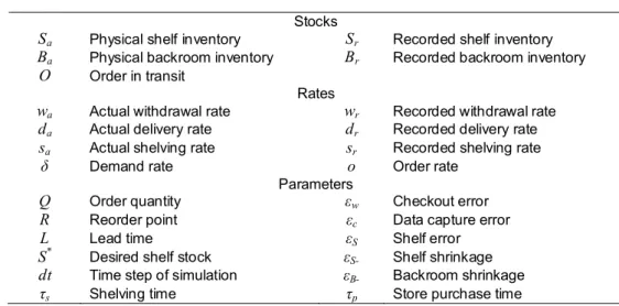
Table 1 Notation

Stocks

Sa Physical shelf inventory Sr Recorded shelf inventory

Ba Physical backroom inventory Br Recorded backroom inventory

O Order in transit

Rates

wa Actual withdrawal rate wr Recorded withdrawal rate

da Actual delivery rate dr Recorded delivery rate

sa Actual shelving rate sr Recorded shelving rate

δ Demand rate o Order rate

Parameters

Q Order quantity εw Checkout error

R Reorder point εc Data capture error

L Lead time εS Shelf error

S* Desired shelf stock εS- Shelf shrinkage

dt Time step of simulation εB- Backroom shrinkage

τs Shelving time τp Store purchase time

We present our model using the system dynamics convention, i.e., in continuous time and as a set of nonlinear differential equations, where the change rates represent information or material flows (measured in units/time) and the accumulation of these rates are represented as stocks (measured in units). We keep track of products in three distinct stocks: shelf, backroom, and orders-in-transit. For convenience we drop

the time index t. The shelf stock (Sa) is augmented by the shelving rate (sa) and depleted by the

merchandise withdrawal rate (wa).

a

a a dS

s w

dt   (1)

With enough items on the shelf, the withdrawal rate (wa) will equal the constant demand rate (δ).

Otherwise, the amount withdrawn will depend on remaining stock quantity and the store purchase time (τp), i.e., the time it takes a customer to make a purchase and walk out of the store.

(2)

The shelving rate (sa) is the flow of inventories pulled from the backroom to the shelf. For simplicity,

re-shelving is assumed to be continuous and proportional to the gap between desired shelf stock S* and recorded shelf inventory Sr, and the process is adjusted by the time it takes store associates to identify the

gap and replenish the shelf (τs). The shelving operation is also subject to a physical constraint since the

retailer cannot replenish more than the amount stored in the backroom (Ba). Thus,

(3)

The backroom stock (Ba) is depleted by the shelving rate (sa) and augmented by the delivery rate (da),

which refers to the actual goods shipped to the backroom inside a retail store.

(4)

We assume a reliable supplier, and thus the delivery rate (da) is the order rate (o) with a fixed time delay

L.

(5)

The order-in-transit stock (O) represents the orders that have been placed to the supplier but have not been delivered yet. Accordingly, it is augmented by the order rate (o) and depleted by the delivery rate (da):

(6)

The order rate (o) in a continuous review (Q,R) is activated whenever inventory position, i.e., the sum of recorded inventory on-hand (Ir=Br+Sr) and order-in-transit (O), drops to/below the reorder point

R.

(7)

where dt is the time step of simulation and a very small time interval to reflect the negligible time of placing an order from the automated ordering system. Ind( ) is an indicator function that returns one if the trigger criterion is met.

Equations (1)–(7) capture physical flows of the item from supply line to customers. Under perfect ( , / ) a a p w Min S  * ( r, a) a s s B S S s Min     a a a dB d s dt   ( ) ( ) a t t L d o _ a dO o d dt   ( / ) * ( _r ) o Q dt Ind I OR

store operations, the information flows will be identical to physical flows. Therefore, the recorded shelf stock (Sr) and recorded backroom stock (Br) change rates are just

(8)

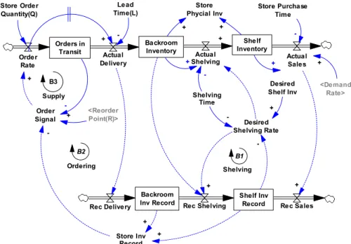
Equations (1)–(8) capture error-free inventory execution. The upper side of Figure 1 exhibits stocks and flows of physical inventories. The bottom side of Figure 1 exhibits stocks and flows of system inventories. The dashed lines in Figure 1 reflect information processing. During normal operation the retailer continuously monitors Ir (the sum of Br and Sr) to place orders to supply line. The retailer also

monitors Sr to take reshelving actions. The shelving follows a goal-seeking structure (Sterman, 2000)

captured in (3), aiming to bring the shelf stock S back to its desired target S* (see loop B1 in Figure 1). The two stocks modeled in (8), together with equations (6) and (7), comprise the ordering mechanism and two feedback loops – ordering (B2) and supply (B3) – aimed at maintaining the desired inventory level in the store.

Fig. 1. Stock and flow diagram of store inventory management

Under perfect store operations, constant demand rate, and deterministic lead time, the system in Figure 1 reaches equilibrium and no lost sales are incurred nor does the system generate IRI (differences the values of the physical stocks and the corresponding information stocks). However, management of retail backroom and shelf involves many activities, and random errors may occur at picking, shelving, labeling, and checkout. Thus, we introduce an array of commonly reported and cited errors to represent





Inv Record _{Rec Shelving Rec Sales} Rec Delivery Store Inv Record + + -+ Orders in Transit Order Rate Actual Delivery -+ <Demand Rate> Store Order Quantity(Q) + Desired Shelf Inv -+ Store Purchase Time -Store Phycial Inv + + Desired Shelving Rate -+ + Shelving Ordering B3 Supply Shelving Time

-more realistic operating conditions.

3.2. Inventory system subject to errors

We modified the equations developed earlier to capture an inventory system subject to five types of random errors, including three asymmetric errors (i.e., shelving error, shelf shrinkage, backroom shrinkage) and two symmetric errors (checkout error, data capture error). Despite being in a continuous-time setting, all errors are transaction-based and multiplicative. The multiplicative error formulation is realistic based on field interviews and technically more robust than additive error

formulation (Khader et al., 2014). The goal of our model is to formally describe the interactions between inventory policies and operational errors and allow us to simulate the effects of these interactions on IRI.

Under imperfect execution, the shelf stock (Sa), in addition of being depleted by the withdrawal rate

wa (Eq. 2), is affected by shelf error and shelf shrinkage. Shelf error (εS) arises when less than desired

quantities are put onto the shelf. Under-shelving is not uncommon since store employees could forget items in the backroom or misplace items (Eroglu et al., 2013). Since in most cases, the retail shelf space for a particular item is fixed, our model excludes the possibility of over-shelving. The exclusion of over-shelving is consistent with our conversation with retail managers and our experience of walking through aisles with retail inventory auditors. The under-shelving error in our model is captured as a fraction of the shelving rate (sa).

Shelf shrinkage (εS-) refers to shelf stock loss caused by shoplifting and unrecorded damaged

products (Lee and Ozer, 2007). In essence, this shrinkage should be a function of the number of items in the shelf (a fraction of the current shelf contents). However, to be consistent with to industry reporting practices (Hollinger, 2009) and our interviewees, we formulate this error as a fraction of the flows out of the stocks (% of sales). Both under-shelving (εs) and shelf shrinkage (εs-) are one-sided (non-negative)

random errors, as they cause direct reduction of available stock. The rate of change of the shelf stock (Sa)

(Eq. 1) in the presence of errors becomes

.

(9)

The backroom is also exposed to undetectable stock loss. Backroom shrinkage (εB-) can be attributed

to unobserved spoilage and employee theft, which is not unusual in the retail sector (Fan et al., 2014). Like shelf-shrinkage, and for the same reasons, we model backroom-shrinkage as a faction of the outgoing flow. Under the fallible shelving operations shown in (9), the backroom stock (Ba) change rate

(Eq. 4) becomes

.

(10)

Similar to shelf error (εS) and shelf shrinkage (εS-), backroom shrinkage (εB-) is a one-sided and

(1 ) ( ) a a S a a S dS s w w dt       (1 ) ( ) a a a S a B dB d s s dt      

non-negative random error.

The formulations of (9) and (10) do not capture the case that the item is taken out of the backroom but never makes it onto the shelf due to ignorance or low engagement. Nonetheless, this error is emulated by backroom shrinkage (εB-) in (10) where the outflow of the backroom stock (Ba) is different from the

inflow to the shelf stock (Sa).

We assume that the processing of inventory information is also subject to errors. The recorded shelf stock (Sr) can deviate from the shelf stock (Sa) because the recorded shelving rate (sr) is distorted by the

data capture error (εc) and the withdrawal rate (wr) is distorted by checkout error (εw). A typical cause of

checkout error is misclassification – scanning two different items as two of the same item. For instance, a customer purchases a chicken-flavored soup and a beef-flavored one. When the employee uses POS scanner to record sales, he may scan one flavor twice instead of scanning the items separately. Such time-saving behavior causes IRI (Raman, 2000). Following how Nachtmann et al. (2010) operationalize errors regarding point-of-sale data records in their simulation, we model information errors as a

symmetric fraction of the withdrawal rate with a uniform distribution around a mean of zero. Under imperfect checkout, the recorded shelf stock change rate (Sr) (Eq. 8) becomes

(11) Note that the recorded shelving rate considers the actual shelving rate (without the shelving errors included) as the base for adjustment for the data capture error. Not only is this assumption consistent with the information that would be available to data entry personnel – assuming that the shelving errors were not intentional – but it also allows for an exploration of the interaction effects of operational and information-processing errors.

The rates affecting the recorded backroom stock (Br) shown in equation (8) are also subject to

information processing errors. Specifically, the outflow – recorded shelving rate (sr) –can deviate from

actual shelving rate (sa) because of data capture error (εc), which occurs when store employees do not

correctly record re-shelving quantities, so the store fails to keep track of the true flow of products. While the recorded delivery rate could also deviate from the actual delivery rate, we left it unaffected for this analysis. In the presence of data capture error, the rate of change of Br in (8) is modified into

(12) Similar to checkout error (εw), we model data capture error (εc) as a symmetric fraction of the

corresponding rate with uniform distribution with zero mean. While our model could capture random errors with any known distribution, the uniform distribution setup is consistent with prior simulation studies that model random errors in system inventory levels (Angulo et al., 2004; Waller et al., 2006;

(1 ) (1 ) r r r a c a w dS s w s w dt       (1 ) r r r a a c dB d s d s dt     

Nachtmann et al., 2010).

Note that consistent with the goals for the model, i.e., to assess the impact of different sources of error, the model does not contain the structure to capture the traditional mechanisms to correct IRI: inventory auditing policies and discovery of shelf stockouts by walking around. While these efforts certainly have an effect on the resulting magnitude of IRI, we justify this model boundary choice by observing that any reasonable implementation of these efforts would make them proportional to the IRI level, regardless of its source. Fixing IRI through audits only sets IRI back to zero at a point of time (i.e., interrupts the growth of IRI) and does not affect the underlying execution errors that persist to make IRI re-accumulate after record reconciliation. Thus, the inventory correction efforts would not have an impact on the relative impact of different operational error sources.

The performance metric – IRI – is the average absolute difference between physical (Ia) and system

inventory levels (Ir) over the simulation horizon. Our focus on absolute deviation is consistent with prior

studies (e.g., DeHoratius and Raman, 2008), and the average is more reliable than a single snapshot of IRI at a point of time. The IRI metric is calculated as

(13)

where T is the length of simulation. We also keep track of shelf-OOS (out-of-stock) ratio – the total duration of Sa being empty relative to T. Shelf-OOS ratio is a relevant metric that helps us better explain

the impact of errors on IRI and defined as

. (14)

3.3. Experimental design

We built the model using VENSIM DSS (Ventana Systems, 2010) and simulated the model using Euler integration method for 360 days with an integration interval (dt) of 0.03125. Based on interviews with retail executives who provided data for our study, we set the model parameters as follows: δ=10 units/day,

Q=100 units, Sa(0)=S *

=50 units, τt=0.125 day, and τs=0.25 day. The reorder point R is S *

+δ*(Safety Coverage+L)= (50+10*(3+3))=110. We assume initial inventory records to be accurate (i.e., Br(0)=Ba(0)

and Sr(0)=Sa(0)) and Ia(0)=S*+R. Note that those parameter values were not set for optimal restocking

decisions (there are no cost considerations in our model), but selected to eliminate shelf-OOS under normal operations. Specifically, the desired shelf level (S*) is set to be five times the daily demand, and reorder point (R) includes safety coverage despite the fact that our model has deterministic demand and reliable suppliers. The findings and insights are qualitatively the same given different parameter values. We tested the model under extreme conditions and a variety of scenarios (Forrester and Senge, 1980;

0| ( ) ( ) | T a r I t I t dt T 





Sterman, 2000). The model behavior is not affected by changes in simulation interval, and the main results are robust to changes in the assumptions for demand – i.e., introducing a random element on the demand, or changing its relative magnitude.

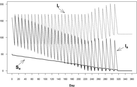
As an illustration of model behavior, we report in Figure 2 the simulation results of a store that experiences shelf and backroom shrinkage. The figure shows the behavior of actual (Ia) and recorded

inventory levels (Ir), as well as the shelf inventory position (Sa). As a result of the shrinkage, the actual

inventory position drops below the recorded inventory. Since the recorded position is used to make shelving (and purchasing) decisions, the amount of inventory in the shelf drops. Eventually the shelf empties (day ~320) and the system falls into the “freezing” scenario that has been reported in previous works (Kang, 2004; Kang and Gershwin, 2005), i.e., the ordering mechanism is not triggered (frozen) as

Ir is still greater than the reorder point R and there are no additional sales to diminish it. The rise in Ir over

time is another known attribute of “freezing” in which each time shrinkage errors occur, the gap between

Ir and Ia grows. Since the reorder quantity is a fixed Q, the accumulation of error makes Ir rise to a point

where Ir stays above R and remains unchanged (Kang and Kershwin, 2005).

Fig. 2. Effect of shrinkage on inventory and shelf stocks†

†Illustration assumptions εS ~ Uniform(0, 0.03) and εB ~ Uniform(0, 0.04)

In line with prior simulation studies related to IRI (e.g., Fleisch and Tellkamp, 2005; Waller et al., 2006; Nachtmann et al., 2010), we employ a full factorial design with three levels of experimental factors to evaluate principal and interaction effects of multiple errors on IRI. Documentation of the full model and simulations runs, according to system dynamics standards (Martinez-Moyano, 2012; Rahmandad and Sterman, 2012), are available in the electronic supplement of this paper.

Table 2 reports the levels of the errors that create variations in the system. We set the experimental values of the five random errors based on interviews with retail managers. For the shelf error, we could

not find reference values from the literature and set the values following managers’ estimates. Although Kang and Gershwin (2005) and Rekik et al. (2009) tested the impact of shrinkage in a range from 1% to 7% of inventory flows, we found these estimates to be too high for our research sites. In line with our interviewees’ responses and the National Retail Security Survey (Hollinger, 2009), we restricted the range of each shrinkage error within 0% to 2% of sales, for a combined expected shrinkage as high as 4% of sales. As for the two information-related errors, checkout and data capture, we specify symmetric and uniform distributions following prior studies that use error terms from +/– 5% to +/– 15% (Waller et al., 2006; Nachtmann et al., 2010), although we limited the worst case scenario to +/– 10% error, which was deemed more reasonable by our interviewees. This reduced error range is consistent with the checkout inaccuracy estimated by Zabriskie and Welsch (1978) and the standard deviation of the resulting

distribution is similar to the one used by Sahin and Dallery (2009). The full factorial design has a total of 35=243 cases and we replicated each scenario 50 times to ensure stable statistical results.

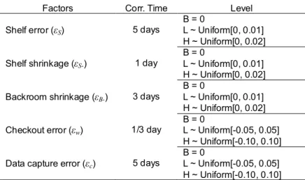
Table 2 Factors and experimental levels for simulation

Factors Corr. Time Level

B = 0

Shelf error (εS) 5 days L ~ Uniform[0, 0.01]

H ~ Uniform[0, 0.02] B = 0

Shelf shrinkage (εS-) 1 day L ~ Uniform[0, 0.01]

H ~ Uniform[0, 0.02] B = 0

Backroom shrinkage (εB-) 3 days L ~ Uniform[0, 0.01]

H ~ Uniform[0, 0.02] B = 0

Checkout error (εw) 1/3 day L ~ Uniform[-0.05, 0.05]

H ~ Uniform[-0.10, 0.10] B = 0

Data capture error (εc) 5 days L ~ Uniform[-0.05, 0.05]

H ~ Uniform[-0.10, 0.10] B: Base; L: Low; H: High

The introduction of random errors on continuous time models like ours, however, requires special treatment since the numbers generated by random functions are independently and identically distributed (white noise). However, calling these functions on every simulation time step results on an oversampling of the independent process and yields stochastic disturbances with constant power spectral density, that, while having the appropriate distribution properties (correct mean and standard deviation), might be changing too quickly relative to the underlying process generating the disturbances. In reality, the processes generating the disturbances have some inertia, as real quantities cannot change infinitely fast and the future values of the disturbance depend on its history. Realistic stochastic processes with

persistence are called “pink noise” and are characterized by a correlation time that determines the historic window that anchors the future values of the stochastic distribution (i.e., the inertia). We adopt the pink

noise structure to model random execution errors as suggested by Sterman (2000).1 We determine the correlation time τε (i.e., inertia) in the pink noise structure for the errors in our model based on each

error’s process characteristics. We set the correlation time of 5 days for the shelving (εS)and data capture

(εc) errors since these operations take place simultaneously and with this expected frequency. Given that

checkout errors are related to the operators, we assume a correlation time of one shift for the checkout errors (εw). As for the two shrinkage errors, we posit that the correlation time for shelf shrinkage (εS-) is

smaller than the correlation time for backlog shrinkage (εB) since the former is likely to be attributed to

mishaps on the shop floor with intense customer contact, while the latter is caused by staff theft or operational errors. Accordingly, we set these correlation times to one and three days respectively. We discuss the effect of these distribution and correlation time assumptions when analyzing our experimental results below.

3.4. Results and analysis

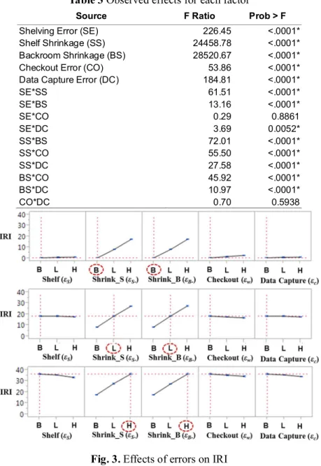
We analyze simulation results using analysis of variance (ANOVA) by least-square fit (Ye et al., 2000) and assess the significance of each experimental factor using an F-test, which is widely used in simulation studies (Nachtmann et al., 2010). Table 3 shows the F-Ratios and p-values for the main effect of the five types of errors and the second order interactions on Average |IRI|.2 All of the main effects are statistically significant and the adjusted R2 for the full model is 0.90. Figure 3 shows the response profile, with 95% confidence intervals, for the main effects of each error under the three treatment levels. To illustrate the interaction effects, we plot the response profile under the three experimental levels for the two dominant errors, i.e., shelf and backroom shrinkage.

1

To generate pink noise error that are uniformly distributed, we first generate standard normal random errors (i.e., white noise) every dt and filter the white noise to generate standard normal pink noise. By using standard normal white noise instead of uniform white noise as inputs, this structure improves Sterman (2000) and no longer relies on central limit theorem to generate normally distributed pink noise (Fiddaman, 2010). We transform the standard normal pink noise into uniform[0, 1] pink noise numerically, using the probability integral transform (Rice, 2006) and then rescale into uniform[0, a] or uniform[-a, a].

2 _{We also assessed performance using final IRI (i.e., | I}

Table 3 Observed effects for each factor

Source F Ratio Prob > F

Shelving Error (SE) 226.45 <.0001*

Shelf Shrinkage (SS) 24458.78 <.0001*

Backroom Shrinkage (BS) 28520.67 <.0001*

Checkout Error (CO) 53.86 <.0001*

Data Capture Error (DC) 184.81 <.0001*

SE*SS 61.51 <.0001* SE*BS 13.16 <.0001* SE*CO 0.29 0.8861 SE*DC 3.69 0.0052* SS*BS 72.01 <.0001* SS*CO 55.50 <.0001* SS*DC 27.58 <.0001* BS*CO 45.92 <.0001* BS*DC 10.97 <.0001* CO*DC 0.70 0.5938

Fig. 3. Effects of errors on IRI

(Top: SS=B & BS=B; Middle: SS=L & BS=L; Bottom: SS=H & BS=H)

Inspection of results reveals that the shrinkage errors (εS- and εB-) dominate the response profile as

they account for 98% of the observed variance. Both error terms are highly significant (F=24458.78,

p-value<0.0001 and F=28520.67, p-value<0.0001 for shelf and backroom shrinkage) and have the

expected direction of increasing the IRI as the shrinkage rates increases. The interaction term between these two errors is also the largest interaction term (F=72.01, p-value<0.0001) and accounts for an additional 0.27% of the explained variance. Note that this dominance of the shrinkage errors is despite the fact that our worst-case scenario for shrinkage rates – 0.02 – is much lower than those tested in previous studies (e.g., Kang and Gershwin, 2005; Rekik et al., 2009). These two errors represent outflows from the physical supply line (one from the shelf stock and one from the backroom stock) that are not reflected on

the information system thus directly affecting product availability but leaving inventory information unchanged. These two errors also account for 38% of the variance observed in shelf-OOS. Finally, it is interesting to note that the magnitude of the impact of these two errors is almost identical, indicating that there is no operational difference on where the shrinkage takes place.

The third operational error – shelving error (εS) – is statistically significant (F=226.45,

p-value<0.0001) but much less impactful than the two asymmetric shrinkage errors (it explains only

0.42% of the observed variance in IRI). The impact of the two information-processing errors is also statistically significant (F=53.86, p-value<0.0001 and F=184.81, p-value<0.0001 for checkout error and data capture error) but not substantial (0.44% of the observed variance). To our surprise, these three often-mentioned errors (Rekik et al., 2008; Sahin and Dallery, 2009) are dominated by the two shrinkage errors and reveal interesting interaction effects. As shown in the top panel of Figure 3, when shrinkage errors are absent (B), the other three errors have positive (although weak) effects on IRI. However, their impacts are in the opposite direction (i.e., average IRI is decreasing in the error rate) when shrinkage errors are present (see the middle and bottom of Figure 3). The negative interactions are explained by the fact that the simulated SKU ‘freezes’ more frequently (see Figure 2 above) under higher shrinkage rates. The shelf-OOS likelihood jumps from 0.15 when there are no shrinkage errors (B) to 0.36 when shrinkage rates are set to 0.01 (L), and to 0.63 when both shrinkage rates are set to 0.02 (H) and these differences are highly significant when assessed using the relative risk (Morris and Gardner, 1988) (p-value<0.001 for L/B and p-value<0.001 for H/L). When shrinkage errors result in freezing and there are no inventory transactions, the associated shelving, checkout, and data capture errors are inactive, thus truncating the growth of IRI. Even if the system does not reach persistent shelf-OOS, both sales and shelving flows will still be reduced by both shrinkage errors, thus weakening the overall impact of other three errors on IRI.

Note that the results reported above are robust to changes in the distribution assumptions for the random errors, and to changes in the correlation time for the asymmetric errors. While the average IRI does decrease with the increase in correlation time of the symmetric errors, the relative magnitude of the effects does not change. Please refer to this paper’s electronic supplement for detailed results and discussion of these tests.

The observed results are consistent with the claim that shrinkage is more difficult to tackle than other sources of IRI (Lee and Ozer, 2007) and suggest that retail managers aiming to improve inventory data quality should pay attention to shelf as well as backroom shrinkage. In retrospect, this result is not surprising, as operational errors represent a deviation from the desired product flow and the

disinformation related to these flows, whereas information-processing errors represent only information deviations. IRI is directly associated with information processing and as such, managers may tend to focus on fixing the symptoms by demanding information personnel to be more careful about data capture.

However, our findings suggest that errors arising from physical operations can actually be the underlying causes of IRI and should be focal improvement targets. The electronic supplement also reports results to changes in the error distribution symmetry assumptions that support conjectures about error interactions put forward by Sahin and Dallery (2009) and Nachtmann et al. (2010).

Finally, the interaction profile graphs reveal that there are no strong interaction effects among operational errors in the system. This is confirmed by the fact that the eight (out of ten) statistically significant interaction terms explain only 1% of the observed variance in IRI. By specifying a model that explicitly accounts for conservation of matter and information distortions, we uncover that the effects of all the errors’ interactions on IRI are almost linear. That said, a potential explanation for this lack of interactions is the fact that the model does not contain the reinforcing relationships between labor availability and existing IRI. We explore labor effects on data integrity in the next two sections.

4. Impact of labor availability on IRI

The prevalence of execution errors reflects the retailer’s inability to manage not only its floor but also labor (DeHoratius and Raman, 2007). Evidently, the behaviors and skills of labor affect the occurrence of those five errors that are significantly associated with IRI. For instance, Zabriskie and Welch (1978) show that checkout accuracy is significantly associated with labor experience and attitude. Also, while

transaction errors may be fixed through better scanning technologies, and misplacement/under-shelving may be tackled by shelf audits, the two most impactful shrinkage errors identified from simulation are closely related to employees’ behaviors and monitoring efforts. Shrinkage (especially in the backroom) must be fixed from inside by employees who are capable of meeting process conformance standards. In line with Ton (2009), we posit that an easy way to tackle the primary drivers of IRI is to enhance process conformance by increasing labor capacity in retail stores. Allocating enough labor and retaining a stable mix of full-timers and part-timers relieves employees’ workload and reduces poor execution of prescribed tasks that cause aforementioned errors. However, deploying sufficient labor with adequate skills is something fundamental but unfortunately ignored by retail managers who pursue payroll minimization (Fisher et al., 2009). In this section, we attempt to empirically assess the impact of labor availability on inventory data integrity. We explore this relationship by measuring labor availability in terms of staffing levels and the employees’ experience and training.

Sufficient staffing levels ensure seamless handling of customer services and in-store logistics, both of which are determinants of sales performance. Ingene (1982) finds a positive and linear association between staffing levels and sales volume per store. Three more recent studies (Fisher et al., 2006; Perdikaki et al., 2012; Chuang et al., 2015) suggest that sales volume is a non-decreasing, concave function of staffing levels. While staffing levels are found to positively affect sales performance, understaffing is a norm rather than an anomaly in the retail sector due to the common practice of wage

minimization (Fisher et al., 2009). Oliva and Sterman (2001) show that understaffing in a service context leads to fatigue, corner-cutting, and service quality erosion. Staffing levels also affect conformance quality that reflects how well store employees execute the prescribed processes. Ton (2009) finds that increasing staffing levels is positively associated with process conformance. In addition to its negative impact on service quality and conformance quality, understaffing potentially can undermine data quality. Since understaffing can cause personnel fatigue, hurried/mindless actions, and poor conformance, all the foregoing consequences of understaffing could lead to execution errors discussed in the simulation analysis. Those errors in information-processing and material handling increase the occurrence and magnitude of IRI. Finally, a fundamental approach to tackle IRI is to frequently inspect the shelves — through predefined cycle-counting or intensive random aisle walking. Frequent data audits are only possible when the organization has sufficient workforce so that employees are not overwhelmed with other tasks.

Simple head-count, however, is not enough to account for labor availability, as individuals’ capabilities have an impact on their ability to perform a task. This is particularly salient in the retail industry where, due to volatile customer demands, retailers often bring in less-expensive and more flexible part-time-employees (PTEs) to cover the short-term mismatches between required labor and the capacity available through full-time-employees (FTEs) (Kesavan et al., 2014). However, unlike FTEs, most PTEs receive limited training and do not accumulate as much experience on the job since they are the last to be hired and the first to be dismissed. As a result, PTEs are consistently assigned to supporting tasks such as re-stocking shelves. To date, there is scant evidence on how the mix of FTEs and PTEs affects store performance. A notable exception is Netessine et al. (2010) who find that allocating more FTEs as opposed to PTEs has positive effects on basket values.

The idea that more PTEs may be counterproductive or detrimental to store performance is not only because of lack of training/experience but also due to the fact that PTEs often obtain minimum benefits, have unstable schedules, and consequently, are less committed to their job (Netessine et al., 2010). Such a lack of commitment causes high turnover of PTEs. The high turnover, unfortunately, is exacerbated by the retailers’ efforts to cut wages and eventually causes low process conformance (Ton and Raman, 2010). Ton (2014) calls the practice of cutting labor budgets by myopically hiring more PTEs a “bad job” strategy that creates a vicious cycle of low quality/quantity of people, poor operational execution, and lost sales/profits.

In the following subsections we describe the research setting, data collection, and operationalization of variables we used to explore the structural functional relationship between labor availability,

considering labor mix, and IRI.

4.1.1. Inventory record inaccuracy

We obtained observations over a period of 10 months on IRI, labor, and time-variant (e.g., number of transactions) and time-invariant (e.g., store area) store characteristics from 5 stores of a global retailer of DIY supplies. A typical store has 100,000 square-feet of retail area and carries 33,000 SKUs. Each store has 13 different product sections in which section managers coordinate the stores’ internal operations. A section is a group of related SKUs that are normally placed in close proximity within the store. Section managers are responsible for maintaining the shelves, displaying the product (i.e., order, access, price labels, etc.), re-stocking the shelves from the backroom, and making adjustments to system-generated order decisions. Each section manager also has the autonomy to make labor allocations and variations on those decisions allow us to examine the effect labor availability has on data quality. Each section manager is also responsible for setting a monthly target of inventory counts to ensure data integrity, as all

restocking decisions in the store are driven by an automated replenishment system.

Each of the 13 product sections had its own inspections in which a portion of SKUs with faulty inventory records (i.e.,|Ia-Ir|>0) was detected and corrected on a nearly daily basis. The inspection

intensity varied from day-to-day and was subject to managers’ orders as well as slack in labor capacity. Understandably, these inventory counts have low priority relative to the task of restocking shelves or helping customers and it is not infrequent that the actual counts are only a fraction of the stated goals. When performing shelf inspections, store associates only recorded error corrections along with Ia and Ir

that were useful for manages to diagnose the severity of IRI.

One of the challenges of working with the data was to derive a robust measure for the dependent variable IRI for each store-section-month as category managers gave inspection different priority. Even within the same section, there was high variance in the inspection rate from month to month. For the 5 stores*13 sections*10 months=650 units (from now on a unit refers to a store-section-month), we had a total of 66,525 corrections that can be used to estimate time-variant metrics of IRI. The number of corrections at month t in section j of store i (kijt) ranges from 0 to 1242 with a mean of 102 and a standard

deviation of 152. One potential metric of IRI for each unit is mean absolute deviation (MAD), a simple and useful measure to capture the mean and spread of IRI (DeHoratius and Raman, 2008). However, the small number of correction records in many units (i.e., 200 out of 650 units have less than 30 correction records) makes MAD (i.e., raw IRI average) unreliable. Furthermore, all observed IRI are zero-truncated as only corrections, i.e., |Ia-Ir|>0, were recorded. That is, we do not have record of all the inspections that

were performed but resulted in no correction.

To tackle small-sample biases in many units and the censoring issue, we adopted Bayesian shrinkage3

estimation to make robust mean inferences given a small sample. This method has been used in marketing studies (e.g., Johnson et al., 2004; Shin et al., 2012) and aims to take advantage of information across subsamples. We defined Yijt=(Yijt,1,…, Yijt,m(t)) as a vector of IRI corrections at month t in section j of store i.

We assumed the sampling model p(Yijt |μijt, ) ~ zero-truncated Poisson-inverse Gaussian(μijt, )

following Oliva et al. (2015) who showed that the Poisson-inverse Gaussian distribution is flexible enough to characterize the distribution of IRI at store, section, or subsection levels. Based on the fact that SKUs within a section are more similar and closely related to each other across months than to SKUs randomly sampled from the entire store, we set μijt ~ Normal(θij, ) (Hoff, 2009) and developed a

Bayesian hierarchical model for each store-section (5 stores*13sections). The proposed model does not allow between-store interactions since it is unreasonable to assume that IRI of a store affects IRI of another store. Below is a visualization of the hierarchical model where θij and are hyper-parameters

that define the distribution of the means of the Poison-inverse Gaussians.

The objective of each store-section model above is to estimate a posterior mean μijt for a unit. The

posterior mean is robust in that it allows μijt with a small sample in one month to “borrow” some

information from a larger sample of corrections in the same store-section but from other months. The information sharing also accommodates unknown inspection frequency since it is reasonable to assume proportionality between the number of observed corrections and inventory counts. The model also assumes a common variability parameter for Yijt. Since all corrections are within the same year and

from stores in the sample company with standard procedures, this assumption is reasonable and avoids more complicated parameterization (Hoff, 2009). Note that it is possible to devise a more complicated model that shares information content across 13 sections within each store. However, the model becomes cumbersome as the number of parameters to be estimated in a single model increases from (T+3) to (T+3)*13+m additional hyper-parameters. Our model strikes a balance between quality of estimation and complexity of computation. described in §3. 2 ij  ij2 2 ij  2 ij  2 ij 

We derived the joint conditional distribution based on the set up – for convenience we drop the store (i) and section (j) indices:

(14)

Based on equation (15), we developed a Markov Chain Monte-Carlo (MCMC) (Jackman, 2009) sampling scheme that allowed us to approximate the Bayes IRI average (i.e., posterior means of IRI

E[μij|Yij]) using simulation and derive the full conditional distribution for all model parameters – θ, τ, σ,

and the key parameter μ (see the detailed derivation in the Appendix). The posterior mean vectors E[μij|Yij]

are robust measures of data quality for all units and serve as dependent variables of regression later. Figure 4 shows that the posterior mean differs more from the raw mean when the sample size of a unit is small (e.g., <30). This correction of small sample bias comes from incorporating information from other months and reflects the effect of Bayesian shrinkage. The Bayesian and raw means of IRI become nearly identical when the sample size increases and more information is available.

Fig. 4. Effect of Bayesian shrinkage

Descriptive statistics in Table 4 show significant variability among units. Compared to Raw IRI average, the Bayes IRI average has a higher mean but a significantly smaller variance (p-value<0.001), as would be expected from the shrinkage procedure (Hoff, 2009), which reduces variability by sharing observed information across periods within each store-section. The higher mean is also a direct

consequence of shrinkage as a large number of corrections in a unit have more influence on the resulting value than those units with low number of corrections. Note that the sample size of Raw IRI average and Bayes IRI average is only 617 because for 33 units we have no observed corrections (kijt=0).

4.1.2. Labor availability and controls

We obtained monthly data on total labor hours (LabHrs) allocated to each store-section as well as the

2 2 2 2 2 2 1 1 1 1

( ,...,



   

, ,

,

|

Y

,...,

Y

)

( ) ( ) (







)

(

  

| ,

)

(

|

 

,

)



_

_

P

P

p

P

p

p Y

number of full-time employees (FTEs) and the part-time employees (PTEs) in a store-month. We used the staffing numbers to calculate the fraction of FTEs hours in store labor (FullFr) as FTEs/(FTEs+PTEs*θ). Such a fractional operationalization based the number of persons is common in panel data econometrics and labor economics (McKee and West, 1984; Baltagi, 2006). The parameter θ (0≤θ≤1) reflects the fact that a PTE may not work for as many hours as a FTE does. Based on our interviews with the director of operations and store managers), we set θ=0.5 and estimated the labor availability as the addition of full-time labor (FullTime) as LabHrs*FullFr and part-time labor (PartTime) as LabHrs*(1-FullFr).

Finally, we identified relevant control variables from DeHoratius and Raman (2008) and secured their corresponding data. The first two controls are product variety and inventory density, both of which cause higher environmental complexity and are considered as drivers of IRI. We approximated product variety as the number of SKUs and inventory density as inventory value (€)/store area. Finally, since increased transactions may lead to more checkout errors, we also controlled for the number of

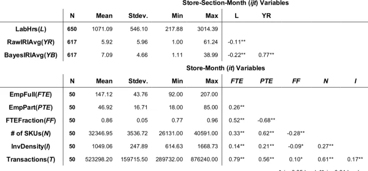
transactions. All these controls were available at the store-month unit of analysis. Table 2 presents

descriptive statistics and pairwise correlations of variables used for empirical estimation.

Table 4 Descriptive statistics and pairwise correlations

Store-Section-Month (ijt) Variables N Mean Stdev. Min Max L YR LabHrs(L) 650 1071.09 546.10 217.88 3014.39

RawIRIAvg(YR) 617 5.92 5.96 1.00 61.24 -0.11**

BayesIRIAvg(YB) 617 7.09 4.66 1.11 38.99 -0.22** 0.77**

Store-Month (it) Variables

N Mean Stdev. Min Max FTE PTE FF N I

EmpFull(FTE) 50 147.12 43.76 92.00 207.00 EmpPart(PTE) 50 46.92 16.71 18.00 85.00 0.26** FTEFraction(FF) 50 0.86 0.05 0.77 0.96 0.52** -0.68** # of SKUs(N) 50 32346.95 3536.72 26131.00 40591.00 0.33** 0.62** -0.28** InvDensity(I) 50 1049.06 247.89 614.63 1668.73 0.14** 0.21** -0.09* 0.27** Transactions(T) 50 523298.20 159715.50 289732.00 876240.00 0.79** 0.56** 0.10* 0.61** 0.17** *sig. 0.05 level; **sig. 0.01 level

4.2. Results and analysis

Considering that IRI is the consequence of deviations in the stores’ operating procedures, we assume that the improvement resulting from any efforts applied to improving the execution of those procedures would follow the well-established-empirical-finding of reducing defects at a constant fractional rate

incremental resources are applied to store’s operations. In our case, we assumed that the ability to perform the store operations correctly is a function of the staffing level, and we specified a non-linear function that characterizes the impact of full-time and par-time labor on IRI

(15)

where the coefficients β1 and β2 indicate the impact of full-time and part-time labor allocation on IRI. A

negative coefficient indicates that IRI is reduced by the availability of that type of labor. X is an array of other factors that may affect IRI.

To econometrically estimate equation (16), we took natural logarithms of (16) and specified a two-way fixed effects (FE) model that considers store-section FE (αij) as well as time effects (Dt)

(Cameron and Trivedi, 2010). FE modeling allows for the store-section-specific FE (αij) to be correlated

with other regressors. Specifying αij helps absorb store- and section-specific time-invariant factors that

may affect IRI. The model is also robust to the unbalanced panel data we have (since we did not have observations of IRI for all units).

. (16)

Table 5 shows the results of de-mean estimation of (17) (Cameron and Trivedi, 2010). The standard errors shown in parentheses are robust to heteroskedasticity and allow for intra-panel correlations. We performed the Wooldridge test (Wooldridge, 2001) and find no evidence of autocorrelation in residuals (ωijt). To test the proposed functional form, we compared our log-linear model specification to the linear

and inverse forms. The log-linear model in eq. (17) achieved a better fit than the other models, and performing the Box-Cox model specification test (Box and Cox, 1964) we failed to reject the log-linear model specification (p-value=0.425) while rejecting the other two.

In model I we included full-time labor hours (FullTime) and part-time labor hours (PartTime) as well as time dummies. The regression is significant (p-value<0.001), explains 60% of the observed variance and coefficients of both variables are significant at the .05 level. The coefficient β1 for full-time

labor is, as expected, negative, indicating that additional FTEs reduce the IRI. β2, however, is positive

indicating that more PTEs increase the IRI. In models II-IV we controlled for product variety

(ProductVar), inventory density (InvDensity), and number of transactions (Transactions). For all models only the control for Transactions is significant. For completeness we also performed random effects (RE) estimation (model V). RE modeling is more efficient but assumes αij to be a random number uncorrelated

with other regressors. We conducted the Hausman test (Wooldridge, 2001) and find no systematic differences between FE and RE estimates. Further, we performed RE estimation (model VI) with Mundlak correction (Mundlak, 1978) for heterogeneity bias by adding two terms for the unit mean of

FullTime and PartTime (Bell and Jones, 2015). The results of model VI are consistent with those from

1 2

exp( )

IRI  FullTime PartTimeπX

1 1 1

2 3

ln( )

ijt ij ijt ijt it

it it t ijt

BayesIRIAvg FullTime PartTime ProductVar

InvDensity Transactions D

   

  

    

ordinary RE modeling (model V) and Transactions is still the only significant control.

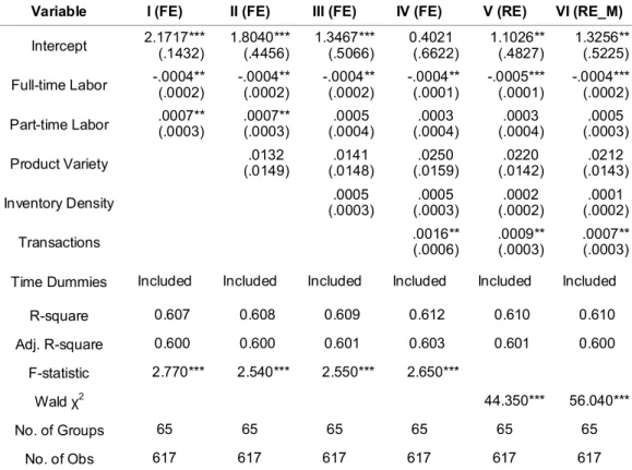
Table 5 Parameter estimates of panel data models

Variable I (FE) II (FE) III (FE) IV (FE) V (RE) VI (RE_M)

Intercept 2.1717*** _(.1432) 1.8040*** _(.4456) 1.3467*** _(.5066) 0.4021 _(.6622) 1.1026** _(.4827) 1.3256** _(.5225) Full-time Labor -.0004** _(.0002) -.0004** _(.0002) -.0004** _(.0002) -.0004** _(.0001) -.0005*** _(.0001) -.0004*** _(.0002) Part-time Labor .0007** _(.0003) .0007** _(.0003) .0005 _{(.0004) (.0004)} .0003 _(.0004) .0003 _(.0003) .0005 Product Variety _(.0149) .0132 _(.0148) .0141 _(.0159) .0250 _(.0142) .0220 _(.0143) .0212 Inventory Density _(.0003) .0005 _(.0003) .0005 _(.0002) .0002 _(.0002) .0001 Transactions .0016** _(.0006) .0009** _(.0003) .0007** _(.0003)

Time Dummies Included Included Included Included Included Included

R-square 0.607 0.608 0.609 0.612 0.610 0.610 Adj. R-square 0.600 0.600 0.601 0.603 0.601 0.600 F-statistic 2.770*** 2.540*** 2.550*** 2.650*** Wald χ2 44.350*** 56.040*** No. of Groups 65 65 65 65 65 65 No. of Obs 617 617 617 617 617 617

*sig. 0.1 level; **sig. 0.05 level; ***sig. 0.01 level

The estimates for the two labor components are stable across all models, but part-time labor becomes insignificant when inventory density and transactions are included in the model. According to our field interviews, most PTEs were brought in to assist shelf restocking operations in busy season and the number of PTEs varied month by month, which is supported by a high ratio of within variance to total variance (0.60). However, each section has a stable base level of FTEs and the variance between sections is much larger than the variance within sections, yielding a within-to-total variance ratio of 0.02. The drop in significance of PartTime is explained by the inclusion of controls with a relatively high within-to-total variance ratio, i.e., inventory density (0.63) and Transactions (0.15). Nevertheless, the remaining positive estimates of PartTime are consistent with store managers’ perceptions that PTEs are not as well trained and more likely to make mistakes that cause IRI (e.g., grab the wrong SKU from the backroom or place a particular SKU in the wrong place).

As a final check, we tested alternative values of θ for FullFr=FTEs/(FTEs+PTEs*θ) as different θs would cause slight variations in the FullTime and ParTime estimated coefficients. We re-estimate the FE and RE models for each θ in the relevant range of [0.3, 1.0] with an increment of 0.005. The results

remain unchanged and still provide significant evidence of the negative effect of full-time labor on IRI and the non-significant effect (when controls are included) of part-time labor on IRI.

5. Impact of IRI on Labor Availability

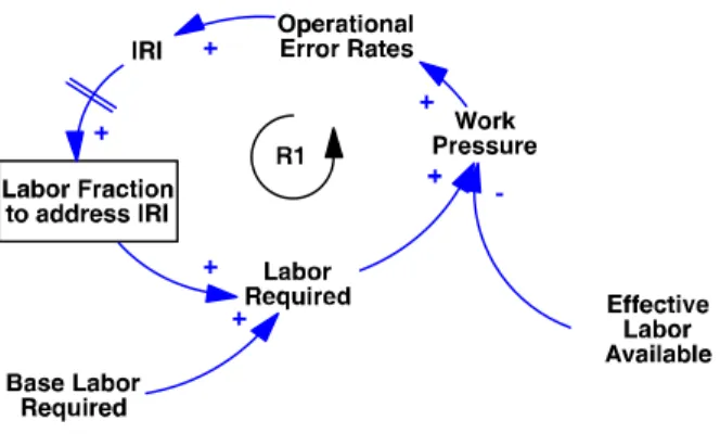
The results from the previous section provide clear evidence that labor availability has an effect of IRI. Furthermore, it is reasonably easy to identify scenarios where IRI, or its consequence, shelf-OOS, could have an impact on the workload of store employees. For example, as discussed in §3, once IRI is present, the restocking system becomes unreliable, increasing the probability of shelf-OOS. Empty shelves translate into confused or angry customers that interrupt normal operations and require special attention through help with searches (either physical or in the computer system), trips to the back room, or placing orders for the missing SKUs. Eventually, high IRI will trigger a response from management that will require employees to perform inventory counts or walk-by shelf inspection. All these activities represent distractions from ‘regular’ operations, thus reducing the labor available to perform them. As per §4, lower labor availability translates into even higher IRI, thus creating a reinforcing loop. Figure 5 operationalizes this reinforcing loop (R1) through the construct of work pressure – the ratio of labor required to effective labor available (Oliva, 2001).

Fig. 5. IRI-Induced work pressure

Nevertheless, it is hard to imagine a situation where this reinforcing loop would run out of control and all employees will be responding to IRI-created work. Customers, for one, would quickly realize that the establishment is not the best option for their purchases and would search for alternative retailers. This would reduce the amount of base labor required to handle regular traffic and would bring work pressure back to normal operating range. However, a quick inspection of the shape and strengths of the links in loop R1 reveals that the gain of this loop saturates very quickly as only a limited fraction of total labor goes into IRI activities.4 Specifically, to assess the gain of the loop around the backlog-shrinkage error,

4

The gain of a link is defined as the ratio of the output to the input, and the gain of a loop is the product of all the link gains in the loop. A reinforcing loop has a positive gain, but to create exponential growth the gain has to be greater than one.