Vehicle Speed Estimation and Forecasting Methods Based on Cellular Floating Vehicle Data

sciences

Vehicle Speed Estimation and Forecasting Methods

Based on Cellular Floating Vehicle Data

Wei-Kuang Lai1,†, Ting-Huan Kuo1,* and Chi-Hua Chen2,3,4,5,†

1 _{Department of Computer Science and Engineering, National Sun Yat-sen University, No. 70, Lienhai Road,} Gushan District, Kaohsiung 804, Taiwan; [email protected]

2 _{Telecommunication Laboratories, Chunghwa Telecom Co., Ltd., No. 99, Dianyan Road, Yangmei District,} Taoyuan 326, Taiwan; [email protected]

3 _{Department of Information Management and Finance, National Chiao Tung University,} No. 1001 University Road, East District, Hsinchu 300, Taiwan

4 _{Department of Communication and Technology, National Chiao Tung University, No. 1001 University Road,} East District, Hsinchu 300, Taiwan

5 _{Department of Electrical and Computer Engineering, National Chiao Tung University,} No. 1001 University Road, East District, Hsinchu 300, Taiwan

* Correspondence: [email protected]; Tel.: +886-7-5252-000 (ext. 4301); Fax: +886-7-5254-301 † These authors contributed equally to this work.

Academic Editor: Antonio Fernández-Caballero

Received: 9 November 2015; Accepted: 25 January 2016; Published: 5 February 2016

Abstract:Traffic information estimation and forecasting methods based on cellular floating vehicle data (CFVD) are proposed to analyze the signals (e.g., handovers (HOs), call arrivals (CAs), normal location updates (NLUs) and periodic location updates (PLUs)) from cellular networks. For traffic information estimation, analytic models are proposed to estimate the traffic flow in accordance with the amounts of HOs and NLUs and to estimate the traffic density in accordance with the amounts of CAs and PLUs. Then, the vehicle speeds can be estimated in accordance with the estimated traffic flows and estimated traffic densities. For vehicle speed forecasting, a back-propagation neural network algorithm is considered to predict the future vehicle speed in accordance with the current traffic information (i.e., the estimated vehicle speeds from CFVD). In the experimental environment, this study adopted the practical traffic information (i.e., traffic flow and vehicle speed) from Taiwan Area National Freeway Bureau as the input characteristics of the traffic simulation program and referred to the mobile station (MS) communication behaviors from Chunghwa Telecom to simulate the traffic information and communication records. The experimental results illustrated that the average accuracy of the vehicle speed forecasting method is 95.72%. Therefore, the proposed methods based on CFVD are suitable for an intelligent transportation system.

Keywords: vehicle speed estimation; vehicle speed forecasting; cellular floating vehicle data; intelligent transportation system; cellular networks

1. Introduction

In recent years, the usage and improvement of mobile techniques have been growing for a variety of real-life applications. For instance, many intelligent transportation systems (ITSs) and services have been designed and developed by several enterprises [1–4]. For the development of ITSs, studying how to collect the traffic information efficiently is a really important topic. The case studies of cooperative intelligent transportation systems (C-ITS) [2,3] and connected-vehicle technology [4] developed real-time traffic information collection methods and evaluated traffic status. Furthermore,

Gao et al. [1] considered traffic status to predict travel time for the design of a navigation system and the avoidance of traffic jams.

ITSs have three kinds of popular position collection approaches, which are the vehicle detector (VD), the reports of global positioning system (GPS)-equipped probe cars and cellular floating vehicle data (CFVD). VD is a sensor based on the techniques of active infrared/laser, magnetic, radar or video to regularly detect vehicles on a road for the analysis of time mean speed and traffic flow [5,6] GPS-equipped probe cars can periodically report their location information to a server for computing the space mean speed [7]. CFVD, which is obtained by tracking the network signals of the mobile station (MS) in the car, can be analyzed to estimate the traffic information (e.g., traffic flow, vehicle speed and traffic density) [5]. The advantages and limitations of these three methods are illustrated in the following paragraphs.

The establishment cost and maintenance fees of VDs were discussed and analyzed in some studies from different countries [8]. For instance, the Texas Transportation Institute spent 43,500 U.S. dollars to install video image vehicle detection systems (VIVD) for the detection of real-time traffic information in 2002. The Ministry of Transportation and Communications in Taiwan spent 75,873 U.S. dollars to establish one VD per each kilometer on Taiwan Highway No. 1 for the collection of real-time road information [9]. However, the maintenance fees of VD solutions are really high because the damage of VD usually result by the environmental factors.

Some studies discussed traffic collection and estimation methods based on the reports of GPS-equipped probe cars, which were compared to the traffic information from VDs for the evaluation of traffic estimation accuracies. For instance, Cheu et al. [10] showed that the lower error rate of space mean speed estimation (less than 3%) can be obtained with enough active probe vehicles. Herrera et al. [10] showed that GPS-equipped probe vehicles periodically recorded their speeds and locations in practical environments for traffic information estimation. Furthermore, their study suggested that a 2%–3% penetration of GPS-equipped probe vehicles is enough to provide accurate measurements of space mean speed. However, the cost of deployment of GPS-equipped probe cars is very expensive for reaching a penetration rate of 2%–3% [10,11].

CFVD can be obtained by tracking MS signals (call arrival (CA), handover (HO), double handover (DHO), normal location update (NLU) and period location update (PLU)), and it can be used for the analysis of traffic status [12,13]. Furthermore, the International Telecommunication Union (ITU) indicated that the handphone penetration rate is more than 100% in many countries [14], and the penetration rate is high enough to assume that everyone has a handphone. Therefore, some studies assumed one handphone in one vehicle. For instance, Lin et al. [9] analyzed two HO locations based on the location service (LCS) as CFVD to estimate the real-time travel time and real-time vehicle speed between HO locations. Their experimental results indicated that the accuracy of the proposed traffic information estimation method was high. However, due to tracing the routes of each MS, a higher computation power is required, and privacy threats may exist. Moreover, future traffic information forecasting based on CFVD has not been investigated.

Therefore, this study proposes analytic models and traffic information estimation methods based on CFVD to obtain a low-cost solution for ITS. The proposed analytic models are used to analyze the relationship between traffic information (e.g., traffic flow, traffic density and vehicle speed) and the amount of cellular network signals (e.g., HO, NLU, CA and PLU). Then, traffic information can be estimated based on the proposed analytic models and CFVD. Furthermore, a vehicle speed forecasting method based on a back-propagation neural network (BPNN) algorithm is proposed to analyze the estimated vehicle speeds from CFVD and to predict the future vehicle speed for road users.

The rest of this study is organized as follows. Section2discusses the related studies and techniques of traffic information estimation and forecasting methods. Section3purposes vehicle speed estimation and forecasting methods based on CFVD. A case study of a highway in Taiwan and experimental results are illustrated and analyzed in Section4. Finally, Section5summarizes the contributions of this study and presents future work.

2. Literature Review

In this section, the techniques of cellular networks, CFVD and traffic information forecasting methods are illustrated in the following subsections. The architecture of cellular networks and mobility management methods are described in Section2.1. Section2.2presents the advantages and limitations of each CFVD method. Finally, traffic information estimation and forecasting methods based on data mining techniques are discussed in Section2.3.

2.1. Cellular Networks

This section presents the network architecture of the Global System for Mobile Communications (GSM)/General Packet Radio Service (GPRS)/Universal Mobile Telecommunications System (UMTS). The components and mobility management (MM) in cellular networks are described as follows.

2.1.1. System Components

The GSM consists of the MS, base transceiver station (BTS), base station controller (BSC), mobile switching center (MSC), home location register (HLR) and visitor location register (VLR). MSs communicate with the network through the BTS and BSC via the A-bis interface (the interface between the BTS and the BSC). The BSC communicates with the MSC via the A (the interface between the BSC and the circuit switched core network) interface, and MSC can connect the calls from the MSs to the public switched telephone network (PSTN). Moreover, the HLR and VLR can provide mobility management and record the location information of the MS [15].

GPRS evolved from GSM and added two new components, which include the serving GPRS support node (SGSN) and the gateway GPRS support node (GGSN). GPRS can establish the data connection with the Internet. However, this study focuses on circuit-switched networks, and the signaling of packet-switched networks is not discussed and analyzed.

The UMTS consists of user equipment (UE), Node B, the radio network controller (RNC) and the components in GSM and GPRS. UEs communicate with the network through Node B and the RNC via the Iub (the interface between the Node B and the RNC) interface. The BSC communicates with the MSC via the IuCS (the interface between the RNC and the circuit switched core network) interface, and the MSC can connect the calls from the UEs to the PSTN [15].

2.1.2. Mobility Management

For MM, the functions related to the management of the common transmission resources may be performed in accordance with the MS/UE. There are two modes, which include idle mode and radio resource (RR) connected mode in RR management.

Idle Mode

In idle mode, the location updating procedures are performed for MM. The location updating procedure is a general procedure, which is used for the following purposes [16].

(1) Normal location updating: NLU is performed when a new location area is entered (European Telecommunications Standards Institute (ETSI), 1995).

(2) Periodic location updating: PLU is performed at the expiration of the timer (ETSI, 1995). (3) International Mobile Subscriber Identity (IMSI) attach: IMSI attach is performed when the MS is

turned on [16].

Radio Resource Connected Mode

In RR connected mode, the handover procedures are performed for MM. The MSC can control the call and the MM of the MS during the call. When MS enters a new cell during a call, the handover procedure is performed to provide good quality RR by the MSC [17]. This study assumes that each

MS in the car can perform the handover procedure in accordance with the specification when the MS enters a new cell during a call.

2.2. Traffic Information Estimation Methods

The techniques of traffic information estimation method based on CFVD can be classified into two groups, which include (1) location services and (2) signal statistics.

2.2.1. Location Services

Several location positioning methods, which were defined in the LCS specification of the 3rd Generation Partnership Project (3GPP), could be grouped into three classes, including: (1) assisted GPS (A-GPS) methods; (2) mobile scan report (MSR)-based location methods; and (3) database lookup methods [18,19].

For A-GPS methods, a GPS component should be equipped in each MS to determine the location of the MS. However, these methods cannot be performed for the MSs without GPS components. Therefore, A-GPS methods are not discussed and applied in this study.

For MSR-based location methods, each MS can send periodically MSR messages (e.g., received signal strength indication (RSSI), round-trip delay and relative delay) to core networks in cellular networks (e.g., Global System Mobile Communications (GSM), Universal Mobile Telecommunications System (UMTS) and Long-Term Evolution (LTE)) [9]. Some studies analyzed the MSR messages to determine the locations of MSs, and these locations can be used to estimate traffic information. For instance, Cheng et al. [9] proposed a fingerprint-positioning algorithm (FPA) based on the k-nearest neighbors (kNN) algorithm to analyze the RSSIs of MSR messages for generating the locations of MS in car, and the average vehicle speed and travel time between two locations of the same MS can be estimated by FPA. Because the interfaces of A-bis and Iub in radio networks should be monitored to retrieve RSSIs for FPA, it is required to have above 10,000 servers to deploy to proceed with recording and analysis by Taiwanese environment. However, core network signals (e.g., CA, HO, NLU and PLU) can be captured via the interfaces of A and IuCS, so only less than 100 servers are needed to be deployed by the Taiwanese environment. The experiment results of FPA showed a high accuracy of vehicle speed estimation, although this method may need higher signaling costs for sending MSR message between MSs and base stations.

For database lookup methods, the information of cellular network signals, which include cell ID, CA, HO and NLU, are considered to generate the mapping table of cell ID, handoff-pair and geographic location. For instance, the cell ID can be retrieved to query the mapping table and to get the geographic location of the queried cell when the CA signal occurs, and the handoff-pair can be retrieved to query the mapping table and to get the geographic location of the queried handoff-pair when the HO signal occurs. When two or more locations of the same MS are determined by database lookup methods, the average vehicle speed and travel time between these locations can be estimated [20]. Birle et al. [21] recorded two handover signals to measure the retention period of each cell, and the time difference between handover signals and the length of the road segment covered by the cell could be analyzed for the estimation of vehicle speed.

The locations of MSs can be precisely determined by using LCS methods, and traffic information can be obtained by the analyses of locations of MSs. However, the location of the MS should be traced, and the power consumption and time complexity of these methods are higher in runtime. Furthermore, the issue of the invasion of privacy should be considered and investigated.

2.2.2. Signal Statistics

Some studies analyzed the relationship between traffic information and the amount of cellular network signals (e.g., NLU, PLU, HO and CA) on the road segments and proposed traffic information estimation methods based on signal statistics. For instance, Caceres et al. [22] collected and counted the handover events, which were triggered when the communicating MSs entered a new cell for traffic

flow estimation. Furthermore, a virtual traffic counter at inter-cell boundaries was proposed to monitor call events in different cells and to estimate traffic flow [23]. A method was proposed to retrieve the NLU events, which were triggered when MSs entered a new location area, and to estimate traffic flow in accordance with the amount of NLU events [24]. For traffic density estimation, a method was proposed to monitor the CA events and to analyze the relationship between traffic density and the amount of CA events [25]. These studies indicated that their proposed methods can estimate traffic information precisely with anonymous MSs.

2.2.3. Summary

Although A-GPS and MRS-based location methods can obtain the precise location information of the MS, heavy computational loads are required for these methods. Database lookup methods may be used to obtain traffic information, but the frequency of vehicle speed report generation is not enough in Taiwan [12]. Moreover, due to tracking of the location of each MS, privacy challenges may arise from using location service methods.

The amount of cellular network signals (e.g., NLU, PLU, HO and CA) from anonymous MSs can be collected and analyzed by signal statistics methods for traffic information estimation. However, long road segments that are covered by a location area are about 10 km, so the traffic information of short road segments cannot be obtained by the analysis of NLU and PLU events. Although the amount of HO events can be used to estimate the traffic condition of short road segments, the variation of HO events may be large in dynamic traffic environments. Therefore, this study proposes a data fusion method based on signal statistics to estimate and forecast traffic information for ITS.

2.3. Traffic Information Forecasting Methods

For traffic information forecasting methods, several studies used data mining techniques (e.g., linear regression [26,27], logistic regression (LR) [28], Bayesian classifier [29,30], k-nearest neighbors (kNN) [31–33], artificial neural network (ANN) [34–37], etc.) to analyze the historical traffic information and obtain the forecasted traffic information.

For traffic information forecasting methods based on regression approaches, some studies used and applied linear regression and LR approaches to predict the future vehicle speed, and the experimental results in these studies showed that the average accuracy of vehicle speed forecasting was higher than 90% for highways [26,28]. However, these regression approaches are unsuitable to analyze the non-linear distribution of data, so the accuracy of the vehicle speed prediction-based regression approach was only 73.3% for an urban road network in [27]. Furthermore, the regression approaches are the special cases of ANN without hidden layers, and the accuracy of the traffic information forecasting method based on ANN may be higher than regression approaches [34–37].

For traffic information forecasting methods based on probability approaches, Bayesian classifier approaches were proposed and used to analyze traffic information and conditions [29], and these approaches could be combined with regression approaches to improve the accuracy of traffic information prediction [30]. However, the assumption and limitation of Bayesian classifier approaches were the independence between input characteristics. Therefore, Bayesian classifier approaches may not be applied to a variety of practical cases.

For traffic information forecasting methods based on the distances between data attributes, a kNN approach was proposed to analyze the previous arrival time, dwell time and delay time for bus arrival time prediction [31,32]. Moreover, some studies used a kNN approach to analyze the relationship of traffic information and weather conditions for the improvement of vehicle speed prediction [33]. Although the results showed that the mean relative errors of using the kNN method were lower, the power consumption and time complexity of the kNN method were higher with big data at runtime.

For traffic information forecasting methods based on ANN, some studies proposed and applied ANN to forecast short-term traffic information, and the experimental results showed that the accuracy of using ANN was better than using other approaches [35–37]. Although a previous study classified

road segments into several road types for reducing ANN models [35], the diverse traffic characteristics of road segments may exist in the same type of road. Moreover, using ANN to analyze CFVD for short-term traffic information prediction has not been investigated. Therefore, this study proposed a traffic information forecasting method based on ANN to analyze and predict the traffic information of each road segment from CFVD.

3. Traffic Information Estimation and Forecasting Methods

The traffic information estimation methods based on CFVD are proposed and analyzed in Section3.1, and the estimated traffic information is adopted as the input parameters for the proposed traffic forecasting method in Section3.2. The details of traffic information estimation and forecasting methods are described as follows.

3.1. Traffic Information Estimation Methods

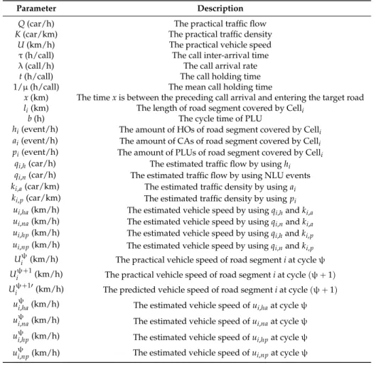
This study proposes some analytic models to estimate traffic flow based on the amount of HOs and NLUs and to estimate traffic density based on the amount of CAs and PLUs. The traffic information estimation method of CFVD is applied to estimate the traffic flow and traffic density. The estimated traffic flow and traffic density are then used for vehicle speed estimation. The notation used in this paper is summarized in Table1. The vehicle speed can be estimated in accordance with traffic flow and traffic density by Equation (1) [19].

Ui“ Qi

Ki (1)

Table 1.The definition of notation. PLU, periodic location update; HO, handover; CA, all arrival; NLU, normal location update.

Parameter Description

Q (car/h) The practical traffic flow K (car/km) The practical traffic density

U (km/h) The practical vehicle speed τ(h/call) The call inter-arrival time

λ(call/h) The call arrival rate

t (h/call) The call holding time

1/µ (h/call) The mean call holding time

x (km) The time x is between the preceding call arrival and entering the target road li(km) The length of road segment covered by Celli

b (h) The cycle time of PLU

hi(event/h) The amount of HOs of road segment covered by Celli ai(event/h) The amount of CAs of road segment covered by Celli pi(event/h) The amount of PLUs of road segment covered by Celli

qi,h(car/h) The estimated traffic flow by using hi qi,n(car/h) The estimated traffic flow by using NLU events ki,a(car/km) The estimated traffic density by using ai ki,p(car/km) The estimated traffic density by using pi

ui,ha(km/h) The estimated vehicle speed by using qi,hand ki,a ui,na(km/h) The estimated vehicle speed by using qi,nand ki,a ui,hp(km/h) The estimated vehicle speed by using qi,hand ki,p ui,np(km/h) The estimated vehicle speed by using qi,nand ki,p

U_iψ(km/h) The practical vehicle speed of road segment i at cycle ψ Uψ`1<sub>i</sub> (km/h) The practical vehicle speed of road segment i at cycle pψ ` 1q U_iψ`11(km/h) The predicted vehicle speed of road segment i at cycle pψ ` 1q

uψ_i,ha(km/h) The estimated vehicle speed of ui,haat cycle ψ uψ_i,na(km/h) The estimated vehicle speed of ui,naat cycle ψ uψ_i,hp(km/h) The estimated vehicle speed of ui,hpat cycle ψ uψ_i,np(km/h) The estimated vehicle speed of ui,npat cycle ψ

3.1.1. Traffic Flow Estimation

This study considers the amount of HOs (hi) and the amount of NLUs (qi,n) to estimate traffic flow (Qi) on the road segment covered by Celli.

Traffic Flow Estimation by Using HO Events

When a call arrives within the coverage area of a cell, the destination (or the originating) MS will be connected if a channel is available. While a communicating MS moves from the coverage area of one cell to the coverage area of another cell, the channel in the old cell is released, and the new cell will provide a channel to the MS if there is a free channel. This process is called a handover.

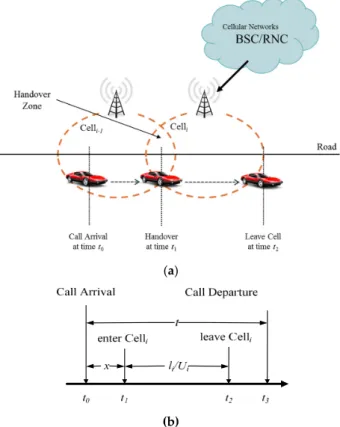
Figure1a illustrates the space diagram for vehicle movement and the handover on a road. Figure1b depicts the timing diagram for the handover on the road segment covered by Celli. The MS in a car performs the call set-up at time t0(in Figure1a,b); then, the MS goes into the handover area of the coverage of Celli´1and Celliat time t1(in Figure1a,b), and the base station controller (BSC) or radio network controller (RNC) will allocate an available channel for the communicating MS. At this moment, if Celli has a free channel, the connection between the MS and Celli will be established successfully. The process is called a handover from Celli´1to Celli.

Appl. Sci. 2016, 6, 47 7 of 20

This study considers the amount of HOs (hi) and the amount of NLUs (qi,n) to estimate traffic

flow (Qi) on the road segment covered by Celli.

Traffic Flow Estimation by Using HO Events

When a call arrives within the coverage area of a cell, the destination (or the originating) MS will be connected if a channel is available. While a communicating MS moves from the coverage area of one cell to the coverage area of another cell, the channel in the old cell is released, and the new cell will provide a channel to the MS if there is a free channel. This process is called a handover.

Figure 1a illustrates the space diagram for vehicle movement and the handover on a road. Figure 1b depicts the timing diagram for the handover on the road segment covered by Celli. The MS in a car

performs the call set-up at time t0 (in Figure 1a,b); then, the MS goes into the handover area of the coverage of Celli−1 and Celli at time t1 (in Figure 1a,b), and the base station controller (BSC) or radio

network controller (RNC) will allocate an available channel for the communicating MS. At this moment, if Celli has a free channel, the connection between the MS and Celli will be established

successfully. The process is called a handover from Celli−1 to Celli.

(a)

(b)

Figure 1. (a) The scenario diagram for vehicle movement and the handover on the road; (b) the timing diagram for the handover on the road segment covered by Celli. BSC, base station controller; RNC, radio network controller.

This study assumes that the call holding time (t) is exponentially distributed with the mean 1/ μ to generate handovers [25]. The average speed of cars is Ui, and the traffic flow is Qi. Furthermore,

the length of road segment covered by Celli is li. Let the variable x be the time difference between t0 and t1, and li/Ui denotes the time difference between t1 and t2. The handover procedure will be

performed when the call holding time (t) is larger than x. Thereby, the amount of handover (hi) on

the road segment covered by Celli can be expressed as Equation (2), and this study can estimate traffic

flow (

q

This study assumes that the call holding time (t) is exponentially distributed with the mean 1{µ to generate handovers [25]. The average speed of cars is Ui, and the traffic flow is Qi. Furthermore, the length of road segment covered by Celli is li. Let the variable x be the time difference between t0and t1, and li/Uidenotes the time difference between t1and t2. The handover procedure will be performed when the call holding time (t) is larger than x. Thereby, the amount of handover (hi) on the road segment covered by Cellican be expressed as Equation (2), and this study can estimate traffic flow (qi,h) by using Equation (3), which is the traffic flow multiplied by the number of HO events.

Appl. Sci. 2016, 6, 47 8 of 19 hi “Qiˆ ş8 x“0Pr pt ą xq dx “Qiˆ ş8 x“0 ş8 t“xµe´µtdtdx “Qiˆ ş8 x“0 ´ ´e´µtˇ ˇ 8 t“x ¯ dx “ Qiˆ ş8 x“0e´µxdx “Qiˆ ˜ ´e´µx µ ˇ ˇ ˇ ˇ 8 x“0 ¸ “ Qi µ (2) qi,h “hiˆ µ (3)

Traffic Flow Estimation by Using NLU Events

In cellular networks, the NLU event is generated when an MS moves from a location area (LA) to another LA. Therefore, traffic flow can be estimated by using the number of NLU events. This study assumes that the actual traffic flow on the road segment covered by Celliis Qiand one MS is in each car (shown in Figure2) [24]. Therefore, the estimated traffic flow qi,n(i.e., the number of NLU events) on the road segment covered by Cellican be calculated as Equation (4), which is the traffic flow multiplied by the number of NLU events.

qi,n“Qi (4)

(

)

(

)



 





Traffic Flow Estimation by Using NLU Events

In cellular networks, the NLU event is generated when an MS moves from a location area (LA) to another LA. Therefore, traffic flow can be estimated by using the number of NLU events. This

study assumes that the actual traffic flow on the road segment covered by Celli is

Q

in each car (shown in Figure 2) [24]. Therefore, the estimated traffic flow qi n, (i.e., the number of

NLU events) on the road segment covered by Celli can be calculated as Equation (4), which is the

traffic flow multiplied by the number of NLU events.

,

i n i

q =Q (4)

Figure 2. The scenario diagram of location update events. LA, location area.

3.1.2. Traffic Density Estimation

For traffic density estimation, this study considers the amount of CAs (ai) and the amount of

periodic location updates (PLUs) (pi) to estimate traffic density (Ki) on the road segment covered by Celli.

Traffic Density Estimation by Using CA events

In cellular networks, a cell is supplied with radio service by vicinal BTSs or Node Bs. The BSC in GSM and RNC in UMTS are responsible for the network control. When a call arrives within the coverage area of a cell, the BSC or the RNC provides a free channel to the MS, and the MS will be connected with the corresponding base station if there is a free channel.

Figure 3a depicts the scenario diagram for vehicle movement and call arrivals on the road. Figure 4b

shows the timing diagram for call arrivals on the road segment covered by a specific Celli. The MS in

a car moving along the road performs the first call at time t0 (in Figure 3a,b) and enters the coverage

area of Celli at time t1 (in Figure 3a,b). The MS performs another call at time t2 (in Figure 3a,b) before

leaving Celli (time t3 in Figure 3a,b), and the call performed by the MS is called a call arrival in Celli.

Figure 2.The scenario diagram of location update events. LA, location area. 3.1.2. Traffic Density Estimation

For traffic density estimation, this study considers the amount of CAs (ai) and the amount of periodic location updates (PLUs) (pi) to estimate traffic density (Ki) on the road segment covered by Celli.

Traffic Density Estimation by Using CA events

In cellular networks, a cell is supplied with radio service by vicinal BTSs or Node Bs. The BSC in GSM and RNC in UMTS are responsible for the network control. When a call arrives within the coverage area of a cell, the BSC or the RNC provides a free channel to the MS, and the MS will be connected with the corresponding base station if there is a free channel.

Figure3a depicts the scenario diagram for vehicle movement and call arrivals on the road. Figure4b shows the timing diagram for call arrivals on the road segment covered by a specific Celli. The MS in a car moving along the road performs the first call at time t0(in Figure3a,b) and enters the coverage area of Celliat time t1(in Figure3a,b). The MS performs another call at time t2(in Figure3a,b)

before leaving Celli(time t3in Figure3a,b), and the call performed by the MS is called a call arrival

in CellAppl. Sci. 2016, 6, x i. 9 of 20

(a) 1st Call Arrival

1st Call Arrival 2nd Call Arrival2nd Call Arrival t

li/Ui Entering Celli

Entering Celli Leaving CellLeaving Cellii

x

t0

t0 tt11 tt22 tt33

(b)

Figure 3. (a) The scenario diagram for vehicle movement and call arrivals on the road; (b) the timing diagram for call arrivals on the road segment covered by Celli.

This study assumes that the call inter-arrival time (τ) is exponentially distributed with the mean

1 /λ to generate call arrivals [25]. The length of road segment covered by Celli is li, and the average

speed of cars is Ui. Therefore, li/Ui denotes the time difference between t1 and t3. This study analyzes

the amount of call arrivals (ai) that occur between t1 and t3 on the road segment covered by Celli. The

amount of call arrivals can be expressed as Equation (5), and Equation (6) indicates that this study

can derive estimated traffic density (ki a, ) from the amount of call arrivals.

[

]

∫

∫ ∫

Traffic Density Estimation by Using PLU Events

1st 2nd

Figure 3.(a) The scenario diagram for vehicle movement and call arrivals on the road; (b) the timing diagram for call arrivals on the road segment covered by Celli.

This study assumes that the call inter-arrival time (τ) is exponentially distributed with the mean 1{λ to generate call arrivals [25]. The length of road segment covered by Celli is li, and the average speed of cars is Ui. Therefore, li/Uidenotes the time difference between t1and t3. This study analyzes the amount of call arrivals (ai) that occur between t1and t3on the road segment covered by Celli. The amount of call arrivals can be expressed as Equation (5), and Equation (6) indicates that this study can derive estimated traffic density (ki,a) from the amount of call arrivals.

ai “QiˆPr rt1ăt2ăt3s “Qiˆ ş8 x“0Pr „ x ă τ ă x ` li Ui  dx “Qiˆ ş8 x“0 ş x` li Ui τ“x λe´λτdτdx “Qiˆ 1 ´ e ´λli Ui λ ñ Qi » — –1 ´ ˆ 1 ´λai Qi ˙ 1 λli fi ffi fl « Qi Ui “Ki, where lim U_iÑ81 ´ e ´1 Ui _“ 1 Ui (5)

ki,a“qi » — –1-ˆ 1-λai qi ˙ 1 λli fi ffi fl « Qi Ui “Ki, where lim UiÑ8 1 ´ e ´ 1 Ui “ 1 Ui (6)

Traffic Density Estimation by Using PLU Events

For mobility management, the MS periodically performs the PLU event for the core network in cellular networks. Some MSs may perform the PLU event across the cell in Figure2. Therefore, the probability models shown in Equations (7) and (8) are proposed to provide estimated vehicle density ki,p(i.e., the number of MS) on the road segment covered by Celliaccording to the number of PLU events. This model had been proven in [24,38], and this study summarizes the assumptions in this model as follows.

‚ The actual vehicle density Ki and traffic speed Ui can be obtained from VD on the road. Furthermore, the length of a road segment covered by the cell is l.

‚ The call arrival rate to a cell is λ, and the call arrival process is assumed to be a Poisson process. ‚ The cycle time of PLU is b, and the number of PLU events is pi.

pi “QiˆPrpPLUq “Qiˆ p3 ´ e´λbq ˆ ˆ e´λb l 2Uib ˙ “Kiˆ p3 ´ e´λbq ˆ ˆ e´λb l 2Uib ˙ (7) ki,p“ pi `3 ´ e´λb˘ ˆ ˆ e´λb l 2Uib ˙ (8)

3.1.3. Vehicle Speed Estimation

In this paper, the vehicle speed is obtained by the estimated traffic flow by using HO events (qi,h), the estimated traffic flow by using NLU events (qi,n), the estimated traffic density by using CA events (ki,a) and the estimated traffic density by using PLU events (ki,p). Based on Sections3.1.1and3.1.2, the estimated vehicle speeds ui,ha, ui,na, ui,hpand ui,np can be expressed as Equations (9)–(12). For instance, the estimated vehicle speed ui,hacan be obtained by using qi,hand ki,a; the estimated vehicle speed ui,nacan be obtained by using qi,nand ki,a; the estimated vehicle speed ui,hpcan be obtained by using qi,hand ki,p; the estimated vehicle speed ui,npcan be obtained by using qi,nand ki,p.

ui,ha“ qi,h ki,a “ » — –1-ˆ 1-λai µhi ˙ 1 λli fi ffi fl ´1 (9) ui,na“ qi,n ki,a “ » — –1-ˆ 1-λai qi,n ˙ 1 λli fi ffi fl ´1 (10) ui,hp“ qi,h ki,p “ µhip3 ´ e´λbq ˆ e´λb l 2Uib ˙ pi (11) ui,np“ qi,n ki,p “ qi,np3 ´ e´λbq ˆ e´λb l 2Uib ˙ pi (12)

3.2. Vehicle Speed Forecasting Method

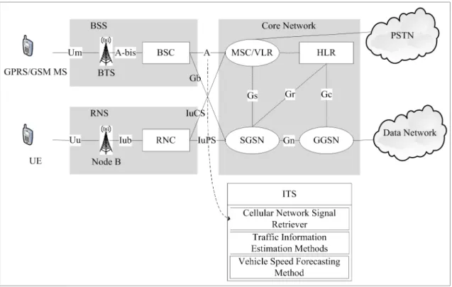
For vehicle speed prediction, a BPNN algorithm is considered to predict the future vehicle speed in accordance with the current traffic information (i.e., the estimated vehicle speeds from CFVD in Section3.1). An intelligent transportation system, which includes a cellular network signal retriever (CNSR), traffic information estimation methods and a vehicle speed forecasting method, has been designed and implemented for traffic information estimation and prediction (shown in Figure4). The ITS can retrieve cellular network signals (e.g., NLU, PLU, HO and CA) via the A interface and the IuCS interface and analyze these signals to estimate traffic information (e.g., traffic flow, traffic density and vehicle speed). Then, the estimated vehicle speed can be adopted as input characteristics into the proposed vehicle speed forecasting method to predict short-term vehicle speed for road user decision. In this subsection, the average vehicle speed of road segment i at cycle ψ is expressed as U_iψ, and the estimated vehicle speed at cycle ψ in accordance with Equations (9)–(12) can be expressed as uψ_i,ha, uψ_i,na, uψ_i,hpand uψ_i,np, respectively. This study collects the values of the current traffic information (i.e., uψ_i,ha, uψ_i,na, uψ_i,hpand uψ_i,np) as the input characteristics of the neurons in the BPNN to predict the future vehicle speed (i.e., U_iψ`1) (see Figure5). Therefore, the number of neurons in the input layer is four. There is one hidden layer, and the output value of the predicted vehicle speed U<sub>i</sub>ψ`11can be obtained by BPNN.

Appl. Sci. 2016, 6, 47 12 of 20

Figure 4. Intelligent transportation system based on the proposed methods.

Figure 5. Vehicle speed estimation based on the back-propagation neural network algorithm.

In the training stage, the historical datasets of cellular network signals from CNSR and traffic information from VDs are collected and calculated the amount of NLU, PLU, HO and CA events. Then vehicle speed can be estimated in accordance with the estimated traffic flows by using NLU and HO events and the estimated traffic densities by using PLU and CA events to obtain the values

of ui haψ, , ui naψ, , ui hpψ, and ui npψ, at

cycle

ψ 1

i

U + _{of road}

segment i at next cycle ( ψ + 1) can be collected by VD. The proposed vehicle speed forecasting

method based on BPNN adopts ui haψ, ,

ψ , i na u , ui hpψ, and ψ , i np

u as input characteristics and Uiψ 1+ as the

output characteristic to train a neural network.

In the runtime stage, the real-time estimated vehicle speeds can be obtained by the proposed traffic information estimation methods based on using CFVD. Then, the estimated vehicle speeds

(ui ha, , ui na, , ui hp, and ui np, ) of road segment i can be adopted into the trained neural network in the

training stage to forecast the short-term vehicle speed at the next cycle.

ψ ha i u_, ψ na i u_, ψ hp i u_, ψ np i u_, ' 1 + ψ i U

Appl. Sci. 2016, 6, 47 12 of 19 Figure 4. Intelligent transportation system based on the proposed methods.

Figure 5. Vehicle speed estimation based on the back-propagation neural network algorithm.

In the training stage, the historical datasets of cellular network signals from CNSR and traffic information from VDs are collected and calculated the amount of NLU, PLU, HO and CA events. Then vehicle speed can be estimated in accordance with the estimated traffic flows by using NLU and HO events and the estimated traffic densities by using PLU and CA events to obtain the values of ui haψ, , ψ , i na u , ui hpψ, and ψ , i np

u at

cycle

i

U + _{of road}

segment i at next cycle ( ψ + 1) can be collected by VD. The proposed vehicle speed forecasting

method based on BPNN adopts ui haψ, , ui naψ, , ui hpψ, and ui npψ, as input characteristics and

ψ 1

i

U + _{as the}

output characteristic to train a neural network.

In the runtime stage, the real-time estimated vehicle speeds can be obtained by the proposed traffic information estimation methods based on using CFVD. Then, the estimated vehicle speeds

(ui ha, , ui na, , ui hp, and ui np, ) of road segment i can be adopted into the trained neural network in the

training stage to forecast the short-term vehicle speed at the next cycle.

ψ ha i u, ψ na i u_, ψ hp i u_, ψ np i u, ' 1 + ψ i U

Figure 5.Vehicle speed estimation based on the back-propagation neural network algorithm.

In the training stage, the historical datasets of cellular network signals from CNSR and traffic information from VDs are collected and calculated the amount of NLU, PLU, HO and CA events. Then vehicle speed can be estimated in accordance with the estimated traffic flows by using NLU and HO events and the estimated traffic densities by using PLU and CA events to obtain the values of uψ_i,ha, uψ_i,na, uψ_i,hpand uψ_i,npat cycle ψ. Moreover, the average vehicle speed Uψ`<sub>i</sub> 1of road segment i at next cycle (ψ + 1) can be collected by VD. The proposed vehicle speed forecasting method based on BPNN adopts uψ<sub>i,ha</sub>, uψ<sub>i,na</sub>, uψ<sub>i,hp</sub>and uψ<sub>i,np</sub>as input characteristics and Uψ`1_i as the output characteristic to train a neural network.

In the runtime stage, the real-time estimated vehicle speeds can be obtained by the proposed traffic information estimation methods based on using CFVD. Then, the estimated vehicle speeds (ui,ha, ui,na, ui,hpand ui,np) of road segment i can be adopted into the trained neural network in the training stage to forecast the short-term vehicle speed at the next cycle.

4. Experimental Results and Analyses

This section adopts the practical traffic information (i.e., traffic flow and vehicle speed) from Taiwan Area National Freeway Bureau as the input characteristics of the traffic simulation program and refers to the MS communication behaviors from Chunghwa Telecom to simulate the traffic information and communication records. The details of the experimental environments are presented in Section4.1. The traffic information estimation and forecasting methods are illustrated in Sections4.2and4.3.

4.1. Experimental Environments

In this study, trace-driven experiments, which consider vehicle movement traces and MS communication traces, are designed to evaluate the traffic information estimation and forecasting methods based on CFVD (shown in Figure6). The inputs of the trace generator include the road conditions (e.g., the length of the road, the number of lanes, the locations of handover points and traffic flows), the vehicle movement behaviors (e.g., vehicles speeds, car following model and lane-changing model) and MS communication behaviors (e.g., call inter-arrival time and call holding time). The output is a trace file, which records the vehicle’s ID, vehicle speed, its CAs, its HOs, its NLUs and its PLUs. For the generation of vehicle movement traces, the practical traffic information, which included traffic flows and vehicle speeds from VDs on National Highway No. 3 in Taiwan during October in 2010, was collected and expressed as the characteristics of road conditions (i.e., traffic flows) and vehicle movement behaviors (i.e., vehicle speeds) for traffic simulation. Furthermore, call holding time is exponentially distributed with the mean 1{µ, and the call inter-arrival time is exponentially distributed with the mean 1{λ in accordance with the mobile communication records from Chunghwa Telecom for

Appl. Sci. 2016, 6, 47 13 of 19

the generation of MS communication traces [13]. Then, vehicle movement and MS communication traces can be generated by a traffic simulation program, VISSIM. Figure7shows nine handover points and nine cells distributed in three location areas on the road from 0–9 km, and the coverage of a cell is 1 km. Moreover, this study assumes that there are nine VDs, which are built in the same locations with handover points for evaluating the traffic information of each road segment covered by a cell.

4. Experimental Results and Analyses

This section adopts the practical traffic information (i.e., traffic flow and vehicle speed) from Taiwan Area National Freeway Bureau as the input characteristics of the traffic simulation program and refers to the MS communication behaviors from Chunghwa Telecom to simulate the traffic information and communication records. The details of the experimental environments are presented in Subsection 4.1. The traffic information estimation and forecasting methods are illustrated in Subsections 4.2 and 4.3.

4.1. Experimental Environments

In this study, trace-driven experiments, which consider vehicle movement traces and MS communication traces, are designed to evaluate the traffic information estimation and forecasting methods based on CFVD (shown in Figure 6). The inputs of the trace generator include the road conditions (e.g., the length of the road, the number of lanes, the locations of handover points and traffic flows), the vehicle movement behaviors (e.g., vehicles speeds, car following model and lane-changing model) and MS communication behaviors (e.g., call inter-arrival time and call holding time). The output is a trace file, which records the vehicle’s ID, vehicle speed, its CAs, its HOs, its NLUs and its PLUs. For the generation of vehicle movement traces, the practical traffic information, which included traffic flows and vehicle speeds from VDs on National Highway No. 3 in Taiwan during October in 2010, was collected and expressed as the characteristics of road conditions (i.e., traffic flows) and vehicle movement behaviors (i.e., vehicle speeds) for traffic simulation. Furthermore, call holding

time is exponentially distributed with the mean 1/ μ, and the call inter-arrival time is exponentially

distributed with the mean 1 / λ in accordance with the mobile communication records from

Chunghwa Telecom for the generation of MS communication traces [13]. Then, vehicle movement and MS communication traces can be generated by a traffic simulation program, VISSIM. Figure 7 shows nine handover points and nine cells distributed in three location areas on the road from 0–9 km, and the coverage of a cell is 1 km. Moreover, this study assumes that there are nine VDs, which are built in the same locations with handover points for evaluating the traffic information of each road segment covered by a cell.

Figure 6. Trace-driven simulation for the traffic information estimations.

Figure 7. The distribution of cells, location areas and vehicle detectors (VDs) in the simulation experiments.

Figure 6.Trace-driven simulation for the traffic information estimations.

4. Experimental Results and Analyses

This section adopts the practical traffic information (i.e., traffic flow and vehicle speed) from Taiwan Area National Freeway Bureau as the input characteristics of the traffic simulation program and refers to the MS communication behaviors from Chunghwa Telecom to simulate the traffic information and communication records. The details of the experimental environments are presented in Subsection 4.1. The traffic information estimation and forecasting methods are illustrated in Subsections 4.2 and 4.3.

4.1. Experimental Environments

In this study, trace-driven experiments, which consider vehicle movement traces and MS communication traces, are designed to evaluate the traffic information estimation and forecasting methods based on CFVD (shown in Figure 6). The inputs of the trace generator include the road conditions (e.g., the length of the road, the number of lanes, the locations of handover points and traffic flows), the vehicle movement behaviors (e.g., vehicles speeds, car following model and lane-changing model) and MS communication behaviors (e.g., call inter-arrival time and call holding time). The output is a trace file, which records the vehicle’s ID, vehicle speed, its CAs, its HOs, its NLUs and its PLUs. For the generation of vehicle movement traces, the practical traffic information, which included traffic flows and vehicle speeds from VDs on National Highway No. 3 in Taiwan during October in 2010, was collected and expressed as the characteristics of road conditions (i.e., traffic flows) and vehicle movement behaviors (i.e., vehicle speeds) for traffic simulation. Furthermore, call holding

time is exponentially distributed with the mean 1/ μ, and the call inter-arrival time is exponentially

distributed with the mean 1 / λ in accordance with the mobile communication records from

Chunghwa Telecom for the generation of MS communication traces [13]. Then, vehicle movement and MS communication traces can be generated by a traffic simulation program, VISSIM. Figure 7 shows nine handover points and nine cells distributed in three location areas on the road from 0–9 km, and the coverage of a cell is 1 km. Moreover, this study assumes that there are nine VDs, which are built in the same locations with handover points for evaluating the traffic information of each road segment covered by a cell.

Figure 6. Trace-driven simulation for the traffic information estimations.

Figure 7. The distribution of cells, location areas and vehicle detectors (VDs) in the simulation experiments.

Figure 7. The distribution of cells, location areas and vehicle detectors (VDs) in the simulation experiments.

4.2. The Evaluation of Traffic Information Estimation Methods

The proposed analytic models were evaluated for the evaluation of traffic flow estimation based on the amount of HOs and NLUs and the evaluation of traffic density estimation based on the amount of CAs and PLUs in Sections4.2.1and4.2.2. Finally, the vehicle speed estimation methods based on the estimated traffic flow and the estimated traffic density were evaluated in Section4.2.3.

4.2.1. The Evaluation of Traffic Flow Estimation

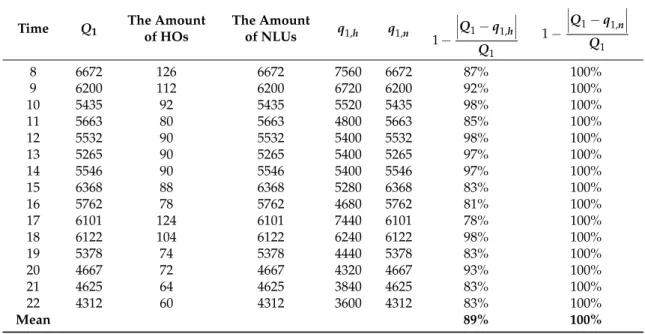
For the evaluation of traffic flow estimation, the simulated amounts of HOs and NLUs from Celli are collected as CFVD to generate qi,hand qi,n. NLU is only performed with MS entering new LA, so the estimated traffic flows are consistence in the same LA in the proposed approach. For instance, the amount of HOs in Cell1(h1) was 126 at 8 a.m. and 9 a.m., so the traffic flow of the first road segment (q1,h) could be estimated as 7560 car/h by utilizing Equation (3) and MS communication behaviors (e.g., the expected value (1{µ) of call holding time is 1 min/call). Furthermore, because 6672 NLUs in Cell1were performed at 8 a.m. and 9 a.m., the traffic flow of the first road segment (q1,n) could be estimated as 6672 car/h according to Equation (4). This study calculated the accuracies of traffic flow estimation as 1 ´ ˇ ˇQ_i´q_i,h ˇ ˇ Qi and 1 ´ ˇ ˇQ_i´q_i,n ˇ ˇ

Qi . Table2shows that the average accuracies of traffic flow estimation of the first road segment between 8 a.m. and 22 p.m. are 89% for the amount of HOs and 100% for the amount of NLUs. As shown in Table3, the comparison of the traffic flow estimation comparisons between q1,hand qi,nindicates that the amount of NLUs is more suitable for traffic flow estimation than the amount of HOs.

Table 2.The accuracies of traffic flow estimation of the road segment covered by Cell1.

Time Q1 The Amount_{of HOs} The Amount_{of NLUs} q1,h q1,n 1 ´ ˇ ˇ ˇQ1´q1,h ˇ ˇ ˇ Q₁ 1 ´ ˇ ˇ ˇQ1´q1,n ˇ ˇ ˇ Q1 8 6672 126 6672 7560 6672 87% 100% 9 6200 112 6200 6720 6200 92% 100% 10 5435 92 5435 5520 5435 98% 100% 11 5663 80 5663 4800 5663 85% 100% 12 5532 90 5532 5400 5532 98% 100% 13 5265 90 5265 5400 5265 97% 100% 14 5546 90 5546 5400 5546 97% 100% 15 6368 88 6368 5280 6368 83% 100% 16 5762 78 5762 4680 5762 81% 100% 17 6101 124 6101 7440 6101 78% 100% 18 6122 104 6122 6240 6122 98% 100% 19 5378 74 5378 4440 5378 83% 100% 20 4667 72 4667 4320 4667 93% 100% 21 4625 64 4625 3840 4625 83% 100% 22 4312 60 4312 3600 4312 83% 100% Mean 89% 100%

Table 3.The accuracies of traffic flow estimation of each road segment.

Cell _{1 ´} ˇ ˇ ˇQi´qi,h ˇ ˇ ˇ Qi 1 ´ ˇ ˇ ˇQi´qi,n ˇ ˇ ˇ Qi Cell1 89% 100% Cell2 76% 100% Cell3 77% 100% Cell4 78% 100% Cell5 70% 100% Cell6 67% 99% Cell7 68% 100% Cell8 70% 100% Cell9 72% 100% Mean 74% 100%

4.2.2. The Evaluation of Traffic Density Estimation

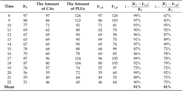
For the evaluation of traffic density estimation, the simulated amounts of CAs and PLUs from Celliare collected as CFVD to generate ki,aand ki,p. For instance, the amount of CAs in Cell1(a1) was 97 at 8 a.m., so the traffic density of the first road segment (k1,a) could be estimated as 97 car/km by Equation (6) and MS communication behaviors (e.g., the expected value (1{λ) of the call inter-arrival time is 1 h/call). Furthermore, because 126 PLUs were performed in Cell1at 8 a.m., the traffic density of the first road segment (k1,p) could be estimated as 128 car/h in accordance with Equation (8) and MS communication behaviors (e.g., call inter-arrival time). This study calculated the accuracies of traffic density estimation as 1 ´

ˇ ˇK_i´k_i,a ˇ ˇ Ki and 1 ´ ˇ ˇK_i´k_i,p ˇ ˇ Ki

. Table4shows that the average accuracies of traffic density estimation of the first road segment between 8 a.m. and 22 p.m. are 91% for the amount of CAs and 81% for the amount of PLUs. As shown in Table5, the results of the traffic density estimation between ki,aand ki,pindicate that the amount of CAs is more suitable for traffic density estimation than the amount of PLUs.

Table 4.The accuracies of traffic density estimation of the road segment covered by Cell1.

Time K1 The Amount_{of CAs} The Amount_{of PLUs} k1,a k1,p 1 ´ ˇ ˇK1´k1,a ˇ ˇ K1 1 ´ ˇ ˇK₁´k_1,p ˇ ˇ K1 8 97 97 126 97 128 99% 67% 9 88 86 112 86 103 97% 83% 10 77 71 92 71 81 93% 95% 11 69 62 80 62 74 90% 92% 12 67 69 90 69 58 96% 87% 13 63 69 90 69 70 91% 89% 14 67 69 90 69 74 97% 89% 15 78 68 88 68 99 87% 72% 16 70 60 78 60 85 86% 78% 17 87 96 124 96 105 89% 78% 18 87 80 104 80 105 92% 79% 19 76 57 74 57 97 75% 72% 20 56 55 72 55 60 99% 92% 21 55 49 64 49 70 89% 73% 22 51 46 60 46 64 90% 75% Mean 91% 81%

Table 5.The accuracies of traffic density estimation of each road segment.

Cell 1 ´ ˇ ˇK_i´k_i,a ˇ ˇ Ki 1 ´ ˇ ˇ ˇKi´ki,p ˇ ˇ ˇ Ki Cell1 91% 81% Cell2 88% 75% Cell3 90% 70% Cell4 86% 86% Cell5 84% 75% Cell6 88% 73% Cell7 86% 76% Cell8 87% 84% Cell9 84% 73% Mean 87% 77%

4.2.3. The Evaluation of Vehicle Speed Estimation

For the evaluation of vehicle speed estimation, the estimated vehicle speeds ui,ha, ui,na, ui,hpand ui,npcan be generated via the estimated traffic flow from HO events (qi,h) Equation (3), the estimated traffic flow by using NLU events (qi,n) Equation (4), the estimated traffic density by using CA events (ki,a) and the estimated traffic density by using PLU events (ki,p) by Equations (9)–(12). For instance, the average vehicle speed of the first road segment u1,hacan be estimated as 78 km/h (i.e., u1,ha“q1,h{k1,a) at 8 a.m. in accordance with the estimated traffic flow by using HO events (i.e., q1,h= 7560 car/h) and the estimated traffic density by using CA events (i.e., k1,a= 97 car/km). This study calculated

the accuracies of traffic density estimation as 1 ´ ˇ ˇU_i´u_i,ha ˇ ˇ Ui , 1 ´ ˇ ˇU_i´u_i,na ˇ ˇ Ui , 1 ´ ˇ ˇ ˇUi´ui,hp ˇ ˇ ˇ Ui and 1 ´ ˇ ˇU_i´u_i,np ˇ ˇ Ui

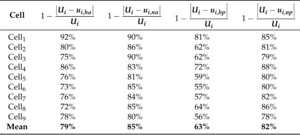
. In accordance with the results in Sections4.2.1 and4.2.2, Table 6shows that the average accuracies of vehicle speed estimation of the first road segment between 8 a.m. and 22 p.m. are 92%, 90%, 81% and 85% for the estimated vehicle speeds ui,ha, ui,na, ui,hpand ui,np, respectively. As shown in Table7, the results of the vehicle speed estimation show that the estimated traffic flow based on the amount of NLUs and estimated traffic density based on the amount of CAs can obtain the highest accuracy of vehicle speed estimation.

Table 6.The accuracies of vehicle speed estimation of the road segment covered by Cell1.

Time U1 u1,ha u1,na u1,hp u1,np 1 ´ ˇ ˇU₁´u_1,ha ˇ ˇ U1 1 ´ ˇ ˇU₁´u_1,na ˇ ˇ U1 1 ´ ˇ ˇ ˇU1´u1,hp ˇ ˇ ˇ U1 1 ´ ˇ ˇU₁´u_1,np ˇ ˇ U1 8 69 78 69 59 52 87% 99% 85% 75% 9 70 78 72 65 60 89% 97% 93% 86% 10 71 78 77 69 67 90% 92% 97% 95% 11 83 77 91 65 76 94% 89% 78% 92% 12 83 78 80 93 96 94% 96% 88% 85% 13 83 78 76 77 75 94% 92% 92% 90% 14 83 78 80 73 75 94% 97% 88% 90% 15 82 78 94 53 64 95% 86% 65% 78% 16 83 78 96 55 68 94% 84% 67% 82% 17 70 78 64 71 58 90% 90% 100% 82% 18 70 78 77 59 58 89% 91% 84% 83% 19 71 78 94 46 55 90% 67% 65% 78% 20 84 79 85 72 78 94% 99% 86% 93% 21 84 78 94 55 66 93% 87% 65% 79% 22 84 78 94 56 67 93% 89% 67% 80% Mean 92% 90% 81% 85%

Table 7.The accuracies of vehicle speed estimation of each road segment.

Cell 1 ´ ˇ ˇU_i´u_i,ha ˇ ˇ Ui 1 ´ ˇ ˇU_i´u_i,na ˇ ˇ Ui 1 ´ ˇ ˇ ˇUi´ui,hp ˇ ˇ ˇ Ui 1 ´ ˇ ˇ ˇUi´ui,np ˇ ˇ ˇ Ui Cell1 92% 90% 81% 85% Cell2 80% 86% 62% 81% Cell3 75% 90% 62% 79% Cell4 86% 83% 72% 88% Cell5 76% 81% 59% 80% Cell6 73% 85% 55% 80% Cell7 76% 84% 57% 82% Cell8 72% 85% 64% 86% Cell9 78% 80% 56% 78% Mean 79% 85% 63% 82%

4.3. The Evaluation of Vehicle Speed Forecasting Method

In this subsection, an LR algorithm and a BPNN algorithm were implemented for the evaluation and comparison of the vehicle speed forecasting method. The estimated vehicle speeds uψ_i,ha, uψ_i,na, uψ_i,hpand uψ_i,npfrom CFVD at cycle ψ were used to predict the future vehicle speed at the next cycle in experiments. For instance, the estimated vehicle speeds of the first road segment u8

1,ha, u81,na, u81,hp and u8_1,npfrom CFVD at 8 a.m., which were 78 km/h, 69 km/h, 59 km/h and 52 km/h, were adopted as input characteristics in the LR and BPNN algorithms. The predicted vehicle speed U₁91could be calculated as 69 km/h by the BPNN algorithm, and the practical vehicle speed U₁9was 70 km/h. Therefore, the accuracy of vehicle speed forecasting could be measured as 98.90% (i.e., 1 ´

ˇ

ˇU₁9´U₁91 ˇ ˇ U₁9 ). Table8shows that the average accuracies of vehicle speed forecasting based on the LR and BPNN algorithms between 8 a.m. and 22 p.m. are 94.82% and 96.01%. As shown in Table9, the results of the vehicle speed forecasting comparisons indicate that the BPNN algorithm is more suitable for predicting the future vehicle speed for ITS.

Table 8. The accuracies of vehicle speed forecasting of the road segment covered by Cell1. LR, logistic regression.

Time Uψ`1_i Forecasted Vehicle_{Speed of LR} Forecasted Vehicle_{Speed of BPNN} The Accuracy_{of LR} The Accuracy_{of BPNN}

8 70 76 69 92.32% 98.90% 9 71 78 73 90.05% 96.32% 10 83 79 77 95.95% 93.26% 11 83 83 81 99.78% 97.30% 12 83 85 86 98.40% 96.86% 13 83 80 80 96.60% 96.74% 14 82 80 80 97.89% 98.18% 15 83 81 78 97.89% 93.95% 16 70 82 79 83.16% 87.91% 17 70 72 73 97.73% 96.19% 18 71 74 75 95.30% 93.91% 19 84 79 81 94.50% 96.52% 20 84 79 80 94.54% 95.47% 21 84 80 84 94.75% 99.93% 22 85 79 86 93.47% 98.76% Mean 94.82% 96.01%

Table 9.The accuracies of vehicle speed forecasting of each road segment. Cell The Accuracy of LR The Accuracy of BPNN

Cell1 94.82% 96.01% Cell2 93.76% 96.29% Cell3 93.42% 95.24% Cell4 92.39% 94.03% Cell5 93.25% 94.72% Cell6 93.59% 97.35% Cell7 92.26% 95.74% Cell8 93.73% 95.19% Cell9 93.84% 96.88% Mean 93.45% 95.72%

5. Conclusions and Future Work

Several studies have reviewed and analyzed how to obtain the traffic information from CFVD. However, they cannot be applied directly to predict the future traffic information in dynamical environments. Therefore, this study proposes analytic models to estimate the traffic flow in accordance with the amounts of HOs and NLUs and to estimate the traffic density in accordance with the amounts of CAs and PLUs. Furthermore, the vehicle speeds can be estimated according to the estimated traffic flows and estimated traffic densities. For vehicle speed forecasting, a back-propagation neural network algorithm is considered to predict the future vehicle speed via the current traffic information. In an experimental environment, this study adopted the practical traffic information from Taiwan Area National Freeway Bureau as the input characteristics of the traffic simulation program and referred to the MS communication behaviors from Chunghwa Telecom to simulate the traffic information and communication records. The experimental results illustrated that the average accuracies of vehicle speed estimation of road segments are 79%, 85%, 63% and 82% for the estimated vehicle speeds ui,ha, ui,na, ui,hpand ui,np, respectively. Moreover, the average accuracy of the vehicle speed forecasting method based on BPNN is 95.72%. Therefore, the proposed methods can be used to estimate and predict vehicle speed from CFVD for ITS.

However, this study assumes that each MS in the car can be filtered and tracked for the collection of cellular network signals (e.g., CAs, HOs, NLUs and PLUs). In the future, filtering out non-vehicle terminals and correctly predicting the routes of vehicle terminals can be investigated in the next study. Furthermore, this study focuses on analyzing the signals from GSM and UMTS networks to estimate the traffic information of the highway for the evaluation of the proposed methods. As the demand for

real-time traffic information increases, the next goal is to estimate and analyze the traffic congestion and transportation delays of urban road segments.

Acknowledgments:The research is supported by the Ministry of Science and Technology of Taiwan under the grant No. MOST 104-2221-E-110-041.

Author Contributions: Wei-Kuang Lai and Ting-Huan Kuo proposed and designed the traffic information estimation and forecasting methods based on CFVD. Chi-Hua Chen and Ting-Huan Kuo performed the proposed methods and reported the experimental results. All of the authors have read and approved this manuscript. Conflicts of Interest:The authors declare no conflict of interest.

References

1. Gao, M.; Zhu, T.; Wan, X.; Wang, Q. Analysis of travel time pattern in urban using taxi GPS data. In Proceedings of the 2013 IEEE International Conference on Green Computing and Communications and IEEE Internet of Things and IEEE Cyber, Physical and Social Computing, Beijing, China, 20–23 August 2013; IEEE: Piscataway, NJ, USA, 2013; pp. 512–517.

2. Green, D.; Gaffney, J.; Bennett, P.; Feng, Y.; Higgins, M.; Millner, J. Vehicle Positioning for C-ITS in Australia (Background Document); Project No. AP-R431/13; ARRB Group Limited: Victoria, Australia, 2013; p. 78. 3. Ansari, K.; Feng, Y. Design of an integration platform for V2X wireless communications and positioning

supporting C-ITS safety applications. J. Glob. Position. Syst. 2013, 12, 38–52. [CrossRef]

4. Schoettle, B.; Sivak, M. A survey of Public Opinion about Connected Vehicles in the U.S., the U.K., and Australia; Report No. UMTRI-2014–10; UMTRI: Ann Arbor, MI, USA, 2014.

5. Jang, J.; Byun, S. Evaluation of traffic data accuracy using Korea detector testbed. IET Intell. Transp. Syst. 2011, 5, 286–293. [CrossRef]

6. Ramezani, A.; Moshiri, B.; Kian, A.R.; Aarabi, B.N.; Abdulhai, B. Distributed maximum likelihood estimation for flow and speed density prediction in distributed traffic detectors with Gaussian mixture model assumption. IET Intell. Transp. Syst. 2012, 6, 215–222. [CrossRef]

7. Hunter, T.; Herring, R.; Abbeel, P.; Bayen, A. Path and travel time inference from GPS probe vehicle data. In Proceedings of the Neural Information Processing Foundation Conference, Vancouver, BC, Canada, December 2009.

8. Middleton, D.; Parker, R. Vehicle Detector Evaluation; Report No. FHWA/TX-03 /2119–1; Texas Transportation Institute, Texas Department of Transportation: Austin, TX, USA, 2002.

9. Cheng, D.Y.; Chen, C.H.; Hsiang, C.H.; Lo, C.C.; Lin, H.F.; Lin, B.Y. The optimal sampling period of a fingerprint positioning algorithm for vehicle speed estimation. Math. Probl. Eng. 2013, 2013, 1–12. [CrossRef] 10. Cheu, R.L.; Xie, C.; Lee, D.H. Probe vehicle population and sample size for arterial speed estimation.

Comput. Aided Civ. Infrastruct. Eng. 2002, 17, 53–60. [CrossRef]

11. Herrera, J.C.; Work, D.B.; Herring, R.; Ban, X.J.; Jacoboson, Q.; Bayen, A.M. Evaluation of traffic data obtained via GPS-enabled mobile phones: The mobile century field experiment. Transp. Res. C Emerg. Technol. 2010, 18, 568–583. [CrossRef]

12. Chang, M.F.; Chen, C.H.; Lin, Y.B.; Chia, C.Y. The frequency of CFVD speed report for highway traffic. Wirel. Commun. Mob. Comput. 2015, 15, 879–888. [CrossRef]

13. Yang, J.Y.; Chou, L.D.; Tung, C.F.; Huang, S.M.; Wang, T.W. Average-Speed Forecast and Adjustment via VANETs. IEEE Trans. Veh. Technol. 2013, 62, 4318–4327. [CrossRef]

14. Maerivoet, S.; Logghe, S. Validation of travel times based on cellular floating vehicle data. In Proceedings of the 6th European Congress and Exhibition on Intelligent Transport Systems and Services, Aalborg, Denmark, 18–20 June 2007.

15. Lin, Y.B.; Pang, A.C. Wireless and Mobile All-IP Networks; John Wiley & Sons: Hoboken, NJ, USA, 2005. 16. ETSI. Digital Cellular Telecommunications System (Phase 2+); Mobile radio interface layer 3 specification, GSM

04.08; European Telecommunications Standards Institute: Sophia Antipolis, France, 1995.

17. ETSI. Digital Cellular Telecommunications System (Phase 2+); Handover procedures, GSM 03.09 version 5.1.0; European Telecommunications Standards Institute: Sophia Antipolis, France, 1997.

18. 3GPP Technical Specification Group (TSG) Services and System Aspects, TS 22.071, Location Services (LCS); Service description; Stage 1 (Release 9), version 9.1.0. 2010. Available online: http://www.3gpp.org/ specifications-groups (accessed on 2 February 2016).

19. Chen, C.H. Traffic Information Estimation Methods Based on Cellular Network Data. Ph.D. Thesis, Department of Information Management and Finance, National Chiao Tung University, Hsinchu, Taiwan, 2013.

20. Ernst, I.; Sujew, S.; Thiessenhusen, K.U.; Hetscher, M.; Rassmann, S.; Ruhe, M. LUMOS-airborne traffic monitoring system. In Proceedings of the 6th International IEEE Conference on Intelligent Transportation Systems, Shanghai, China, 12–15 October 2003; IEEE: Piscataway, NJ, USA, 2003; Volume 1, pp. 753–759. 21. Birle, C.; Wermuth, M. The traffic online project. In Proceedings of the 13th ITS World Congress, London,

UK, 8–12 October 2006.

22. Caceres, N.; Wideberg, J.P.; Benitez, F.G. Review of traffic data estimations extracted from cellular networks. IET Intell. Transp. Syst. 2008, 2, 179–192. [CrossRef]

23. Caceres, N.; Romero, L.M.; Benitez, F.G.; del Castillo, J.M. Traffic flow estimation models using cellular phone data. IEEE Trans. Intell. Transp. Syste. 2012, 13, 1430–1441. [CrossRef]

24. Kuo, T.H.; Lai, W.K.; Chen, C.H. A traffic speed estimation model base on using location update events. In Proceedings of the 9th International Conference on Wireless Communications, Network and Mobile Computing, Beijing, China, 22–24 September 2013.

25. Lai, W.K.; Kuo, T.H.; Chen, C.H.; Lee, D.R. A vehicle speed estimation mechanism using handovers and call arrivals of cellular networks. In Proceedings of the 12th International Conference on Advances in Mobile Computing and Multimedia, Kaohsiung, Taiwan, 8–10 December 2014; pp. 19–26.

26. Chen, W.J.; Chen, C.H.; Lin, B.Y.; Lo, C.C. A traffic information prediction system based on global position system-equipped probe car reporting. Adv. Sci. Lett. 2012, 16, 117–124. [CrossRef]

27. Shan, Z.; Zhao, D.; Xia, Y. Urban road traffic speed estimation for missing probe vehicle data based on multiple linear regression model. In Proceedings of the 16th International IEEE Conference on Intelligent Transportation Systems, Hague, The Netherlands, 6–9 Octomber 2013; IEEE: Piscataway, NJ, USA, 2013; pp. 118–123.

28. Antoniou, C.; Koutsopoulos, H.N.; Yannis, G. Dynamic data-driven local traffic state estimation and prediction. Transp. Res. C Emerg. Technol. 2013, 34, 89–107. [CrossRef]

29. Lu, C.C.; Zhou, X. Short-term highway traffic state prediction using structural state space models. J. Intell. Transp. Syst. Technol. Plan. Oper. 2014, 18, 309–322. [CrossRef]

30. Fei, X.; Lu, C.C.; Liu, K. A Bayesian dynamic linear model approach for real-time short-term freeway travel time prediction. Transp. Res. C Emerg. Technol. 2011, 19, 1306–1318. [CrossRef]

31. Liu, T.; Ma, J.; Guan, W.; Song, Y.; Niu, H. Bus arrival time prediction based on the k-nearest neighbor method. In Proceedings of the Fifth IEEE International Joint Conference on Computational Sciences and Optimization, Harbin, China, 23–26 June 2012; IEEE: Piscataway, NJ, USA, 2012; pp. 480–483.

32. Baptista, A.T.; Bouillet, E.P.; Pompey, P. Towards an uncertainty aware short-term travel time prediction using GPS bus data: Case study in Dublin. In Proceedings of the 15th International IEEE Conference on Intelligent Transportation Systems, Anchorage, AK, USA, 16–19 September 2012; IEEE: Piscataway, NJ, USA, 2012; pp. 1620–1625.

33. Kim, S.; Rim, H.; Oh, C.; Jeong, E.; Kim, Y. Multiple-step traffic speed forecasting strategy for winter freeway operations. Transp. Res. Rec. J. Transp. Res. Board 2015, 2482, 133–140. [CrossRef]

34. Chien, S.I.J.; Ding, Y.Q.; Wei, C.H. Dynamic bus arrival time prediction with artificial neural networks. J. Transp. Eng. 2002, 128, 429–438. [CrossRef]

35. Hodge, V.J.; Krishnan, R.; Austin, J.; Polak, J.; Jackson, T. Short-term prediction of traffic flow using a binary neural network. Neural Comput. Appl. 2014, 25, 1639–1655. [CrossRef]

36. Van Lint, J.W. Reliable real-time framework for short-term freeway travel time prediction. J. Transp. Eng. 2006, 132, 921–932. [CrossRef]

37. Ma, X.; Tao, Z.; Wang, Y.; Yu, H.; Wang, Y. Long short-term memory neural network for traffic speed prediction using remote microwave sensor data. Transp. Res. C Emerg. Technol. 2015, 54, 187–197. [CrossRef] 38. Chang, H.C.; Chen, C.H.; Lin, B.Y.; Kung, H.Y.; Lo, C.C. Traffic information estimation using periodic location

update events. Int. J. Innov. Comput. Inf. Control 2013, 9, 2031–2041.

© 2016 by the authors; licensee MDPI, Basel, Switzerland. This article is an open access article distributed under the terms and conditions of the Creative Commons by Attribution (CC-BY) license (http://creativecommons.org/licenses/by/4.0/).