Spin relaxation dynamics of quasiclassical electrons in ballistic quantum dots with strong spin-orbit coupling

(1)

Spin relaxation dynamics of quasiclassical electrons in ballistic quantum dots

with strong spin-orbit coupling

Cheng-Hung Chang,1,4_{A. G. Mal’shukov,}2_{and K. A. Chao}3

1_{National Center for Theoretical Sciences, Physics Division, 101, Section 2 Kuang Fu Rd., Hsinchu 300, Taiwan} 2_{Institute of Spectroscopy, Russian Academy of Science, 142190 Troitsk, Moscow oblast, Russia}

3_{Solid State Theory, Department of Physics, Lund University, S-223 62 Lund, Sweden} 4_{National Chiao Tung University, Institute of Physics, 300 Hsinchu, Taiwan}

(Received 4 May 2004; revised manuscript received 27 August 2004; published 13 December 2004)

We performed path integral simulations of spin evolution controlled by the Rashba spin-orbit interaction in the semiclassical regime for chaotic and regular quantum dots. The spin polarization dynamics have been found to be strikingly different from the D’yakonov-Perel’ (DP) spin relaxation in bulk systems. Also an

important distinction has been found between long time spin evolutions in classically chaotic and regular systems. In the former case the spin polarization relaxes to zero within relaxation time much larger than the DP relaxation, while in the latter case it evolves to a time independent residual value. The quantum mechanical analysis of the spin evolution based on the exact solution of the Schrödinger equation with Rashba SOI has confirmed the results of the classical simulations for the circular dot, which is expected to be valid in general regular systems. In contrast, the spin relaxation down to zero in chaotic dots contradicts what has to be expected from quantum mechanics. This signals on the importance of quantum effects missed in the semiclas-sical simulations for long time spin dynamics.

DOI: 10.1103/PhysRevB.70.245309 PACS number(s): 72.25.Rb, 72.25.Dc, 73.63.Kv, 03.65.Sq

I. INTRODUCTION

Spin relaxation in semiconductors is an important physi-cal phenomenon being actively studied recently in connec-tion with various spintronics applicaconnec-tions.1 _{In doped bulk} samples and quantum wells(QW) of III-V semiconductors at low temperatures spin relaxation is mostly due to the D’yakonov-Perel’(DP) mechanism.2 This mechanism does not involve any inelastic processes, so that the exponential decay of the spin polarization is determined entirely by the spin-orbit interaction(SOI) and elastic scattering of electrons on the impurities. However, in case of confined systems such as quantum dots(QD) with atomiclike eigenstates, the SOI has been incorporated into the structure of the wave func-tions of the discrete energy levels. Without inelastic interac-tions, an initial wave packet with a given spin polarization will evolve in time as a coherent superposition of these dis-crete eigenstates. Therefore, the corresponding expectation value of the spin polarization will oscillate in time without any decay. To obtain a polarization decay in the QD’s, extra effects have to be introduced into the system, e.g., the inelas-tic interactions between electrons and phonons mediated by the spin-orbit3,4 _{and nuclear hyperfine effects.}3,5,6 Accord-ingly, a spin relaxation in QD’s induced by these effects is a real dephasing process.

Unlike such an inelastic relaxation in QD’s, the DP spin relaxation in unbounded systems seems to be quite a differ-ent phenomenon, because the scattering on impurities is elas-tic and there is no dephasing of the electron wave functions in the systems. However, the spin polarization does decay in time exponentially, as if it would be a true dephasing pro-cess. To explain this phenomenon, let us consider an electron moving diffusively through an unbounded system with ran-dom elastic scatters. This electron is described by a wave

packet represented by a superposition of continuum eigen-states. During a DP relaxation process, the spin expectation value expressed as a bilinear combination of these wave am-plitudes will decay exponentially in time. This process can be easily understood from the semiclassical Boltzmann or Fokker-Planck approach.2 _{Indeed, keeping in mind that the} SOI has the form ␴· h共k兲, where ␴ is the vector, whose components are the three Pauli matrices, and h共k兲 is the effective magnetic field, whose magnitude and direction de-pend on the electron momentum k, one can envision spin relaxation as the spin random walk on the surface of the unit sphere, similar to that in Fig. 1(c). Starting at the north pole, the spin precesses around h共k₁兲 until the momentum direc-tion is changed by a scattering on an impurity. Thereafter, the magnetic field changes its direction to h共k2兲 and the spin continues its precession around this direction. If the spin ro-tation angle between successive scattering events is small, the sequence of such rotations results in a diffusive spreading of the initial polarization.

Returning to QD’s, a natural question emerges: What sort of spin evolution can be generated by the DP mechanism in a ballistic QD whose size is much larger than the electron wavelength at the Fermi surface and where the mean spacing between energy levels is much less thanប/T, where T is the mean time between electron collisions with the boundary? Similar to the example in Fig. 1, the spin evolution in this semiclassical regime can be studied by tracking the spin walk on the sphere, when particles move along the classical trajectories inside the QD’s. Intuitively, one would expect the spin evolution in this case to be similar to the spin random walk governed by the impurity scattering in unbounded samples. However, this expected analogy with the open sys-tem is wrong. Indeed, in an unbounded syssys-tem, the steps of the random walk are uncorrelated. This results in a diffusive

(2)

decay of the spin polarization down to zero for any nonzero SOI. But in case of QD’s, the steps of the random walk on the sphere are correlated due to the confinement of electron trajectories within the dots. As we will show below, such correlations not only lead to a spin relaxation much longer than the DP relaxation in unbounded systems, but also to a nonzero final polarization value at long time for certain quantum dot geometries. Here, we do not take into account the inelastic mechanisms3–6_{which always drive the spin} po-larization to zero in long time. These mechanisms are as-sumed to be absent, because they become inefficient at suf-ficiently low temperatures. By this reason we will also neglect spin relaxation associated with electron-electron col-lisions in doped QW.7

It should be noted that a tendency for slowdown of the DP relaxation in confined geometries has been also found out for disordered quantum wires,8,9_{diffusive two-dimensional}_(2D) strips,10_{near the edge of 2D gas,}11_{and in the recent study on} quantum dots.12 _{Therefore, the strong distinction of the DP} relaxation in QD from that in bulk systems confirms this tendency.

In this paper, we carry out a semiclassical analysis of the DP relaxation in two-dimensional QD’s of various geom-etries, including a circular dot, a triangular dot, a generalized Sinai billiard, and a circular dot with diffusive scattering on the boundary. Note that although such 2D systems are called QD’s, the confinement in the 2D plane does not lead to strong quantization and the electronic motion can be studied semiclassically. We focus on the case of the strong SOI, such

that the characteristic spin orbit length L_so⬅v_F/បh共k_F兲 is not much larger than the dot size L. Such a regime can be real-ized in the InAs based heterostructures for L⬃0.5−1␮m.13 We found that in the short time scale⬃T the spin relaxation dynamics in all geometries shares a common feature: After a fast initial drop during the time interval⬃T, the spin polar-ization continues to oscillate weakly around some value. For weak SOI with LsoⰇL, all residual values for different dot geometries are quite close to one up to the cutoff time of our numerical simulations 共⬃103_T_{兲. For stronger SOI with L}

so

艌L, the initial drop of the spin polarization is considerably

larger compared to the weak SOI regime. The spin evolution after that drop depends on the dot geometry. In the case of circular and triangular dots, which are examples of systems with regular classical dynamics, the corresponding spin po-larizations approach nonzero residual values. However, in the case of chaotic and random systems (e.g., Sinai billiard and circular dot with rough boundaries, respectively), the spin polarizations slowly decrease to zero after that initial drop. But this decreasing is much longer than the DP relax-ation in an unbounded system, in which the mean impurity scattering time is⬃T. For very strong SOI with Lso⬍L, the spin polarization after the initial drop reaches zero and later on oscillates with a large amplitude.

These results clearly demonstrate that the spin evolution in QD’s is qualitatively distinct from the DP spin relaxation in unbounded systems. In order to elucidate the physical ori-gin of this phenomenon, two investigations have been per-formed. First, the spin evolution along a single electron tra-jectory was studied in detail, which provided a clue for understanding the above-mentioned polarization behavior. Second, the residual polarization obtained from the classical simulations for a circular quantum dot was compared with that derived from the exact solution of the Schrödinger equa-tion. A good agreement between the results from these two approaches has been found. However, for QD’s with chaotic and random electron dynamics, the general quantum me-chanical analysis revealed a contradiction to the long time spin evolution observed in our semiclassical simulations.

The paper is organized in the following way. In Sec. II, the general expression of the polarization will be derived for the spin evolution via classical path integrals. In Sec. III, the results of the numerical simulations in different quantum dots will be demonstrated. The quantum mechanical theory for the spin polarization in the circular quantum dot will be presented in Sec. IV, with the calculation in detail shown in the Appendix. Discussion and conclusion will be given in Sec. V.

II. PATH INTEGRALS FOR THE SPIN EVOLUTION

The Hamiltonian of the system

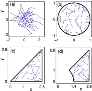
H = H0+␴· h共kˆ兲, 共1兲 consists of the spin independent part H₀, which is the elec-tron kinetic energy plus the 2D confining potential V共r兲, and the spin-orbit interaction. In III-V semiconductor hetero-structures the effective “magnetic” field h共kˆ兲 is given by the FIG. 1.(Color online) (a) Electron motion inside a quantum dot.

The trajectory consists of three straight segments␥1,␥2, and␥3.(b) The corresponding spin evolution on the sxsy plane, which is

pro-jected from(c). (c) The spin evolution induced by the Rashba

(3)

sum of the Bychkov and Rashba14 _{and the Dresselhaus}15 terms. If the z axis is chosen perpendicular to the heterostruc-ture interface, the magnetic field hR contributing to the

Rashba term has two components 关h_Rx共kˆ兲,h_Ry共kˆ兲兴=共␣Rkˆy,

−␣Rkˆx兲, where បkˆ=共បkˆx,បkˆy兲 is the momentum operator. In

the 2D confinement, the magnetic field hDcontributing to the

Dresselhaus term contains both linear and cubic parts with respect to kˆ.16In a[001] oriented QW the linear term has the components 关h_Dx共kˆ兲,h_Dy共kˆ兲兴=共␣Dkˆx, −␣Dkˆy兲. For

heterostruc-tures with a typical⬃10 nm confinement in the z direction, the linear part of hD is usually larger than the cubic part,

except the case of high doping concentration.17_{The Rashba} term is not zero only in heterostructures with asymmetry in their growth direction. This term can be much larger than the Dresselhaus term in the narrow gap InAs based systems.12_In this paper we will study the spin evolution induced by the Rashba term. But, since the SOI Hamiltonians corresponding to the Rashba and the linear Dresselhaus terms can be trans-formed from one to the other by the unitary matrix 共␴x

+␴y兲/

冑

2, our results are also valid for systems in which the

linear Dresselhaus term dominates the SOI.

Let us suppose E_n to be the nth quantized energy level with the eigenfunction␸n, which is a two component spinor.

At zero magnetic field this quantum state is at least doubly degenerate. Let

␺共r兲 = eik·r_{⌽共r − R兲}_␹ _共2兲

be the wave packet created at time t = 0, centered at the point

R, and propagating with the 2D wave-vector k. The function

⌽共r兲 is assumed to be slowly varying within the scale of the

electron wavelength 2␲/ k and normalized, so that the inte-gral兰兩⌽共r兲兩2_d2_{r over the QD volume is equal to 1. The} ini-tial spin polarization P共0兲=兺_␣␤␹_␣*␴_␣␤␹_␤is the sum over the two components␹_␣ of the spinor␹, where␣苸兵1,2其. For t

⬎0, the wave packet evolves in time as

␺共r,t兲 =

兺

n cn␸n共r兲e−i Ent/ប, 共3兲 where cn=

冕

␸n †_共r兲_␺_共r兲d2_r. _共4兲 In terms of ␺共r,t兲 the time dependent spin polarization is expressed as

P共t兲 =

兺

␣␤

冕

␺␣

*_共r,t兲

␴␣␤␺␤共r,t兲d2r, 共5兲

with three components P共t兲=关Px_{共t兲, P}y_{共t兲, P}z_共t兲兴.

For further analysis it is convenient to introduce the re-tarded and advanced Green’s functions

⬘

兲 is the Heaviside function. Using these Green’s functions, the spin-spin correlation function can be defined as

in time

Pi共t兲 =1 2

冕

dr1¯ drn

兺

␣1,␣2,¯

具r,␣兩e−iH共t−t₁兲_兩r 1,␣1典

⫻具r1,␣1兩e−iH共t1−t2兲兩r2,␣2典¯ 具rn,␣n兩e−iH共tn−t⬘兲

⫻兩r

⬘

,␤典共9兲

of the evolution operators e−iH共ti−tj兲 _{within the infinitesimally}

short time intervals共ti− tj兲. Thereafter, the Green’s function

can be expressed as the path integral of T exp

关

_បiS共t − t

⬘

, r , r

⬘

兲

兴

, where the action

S共t − t

⬘

,r,r

⬘

兲=

冕

t⬘ t

冋

m* 2 v 2_共_␶_{兲 − V共r共}_␶_{兲兲 − h} R

冉

m*v共␶兲 ប

冊

␴

册

d␶, 共10兲

is a time integral of the particle Lagrangian evaluated along a trajectory starting from r

By using the saddle point approximation, the path integral in Eq.(9) can be reduced to a sum over all classical trajec-tories␥,18

(4)

Gr共t − t

⬘

,r,r

⬘

兲= 1

⬘

, r , r

⬘

兲 along the classical trajectories. The spin de-pendence part of the Green’s function is represented by the unitary matrix

U共t − t

⬘

,r,r

⬘

兲 = Te−i/ប兰t⬘ t

h_R共m*v共␶兲/ប兲␴ d␶_. _共12兲

Such a decoupling of the spatial and spin degrees of freedom can be done under the assumption that the classical paths are only weakly perturbed by SOI, which is reasonable, when the SOI parameter ␣R is much less than the electron Fermi

, r兲

兴

rapidly oscillates as a function of r with a period given by the Fermi wavelength. However, J, U, and⌽ are slowly varying functions of r. The length scale of J’s variation is given by the dot size. The spatial changes of U are controlled by the spin orbit length Lso=ប/共m*␣R兲, which

is assumed to be much larger than the Fermi wavelength. Therefore, the influence of the SOI on the saddle-point posi-tion can be ignored. The variaposi-tion of⌽ also can be ignored, because this function was assumed to change weakly within the length scale equal to the electron wavelength. Under these approximations, we obtain the saddle-point equation in the form

⳵S0共t,r

⬙

,r兲

⳵r +បk = 0. 共14兲

This equation is the classical equation of motion. It deter-mines the trajectory r = r0关r

⬙

共t兲,p共0兲兴 which passes through the given point r

⬙

共t兲 at the instant t, on condition that at t = 0 the initial momentum was p共0兲=បk. Therefore, the saddle-point r is a particle coordinate at t = 0 belonging to this trajectory. Since the integral over r

⬘

in Eq.(8) is taken around this extremum, the value r

⬘

= r = r₀ are inserted into all slowly varying functions J, U, and⌽.

Further, to calculate the integral over r in Eq. (13), the action S0共t,r

⬙

, r兲 is expanded around r=r0 up to the second order S₀共t,r

⬙

,r兲 + បk = S₀共t,r

⬙

,r₀兲 +1 2 ⳵S₀共t,r

冊

. 共16兲

By using the identity det

冉

⳵r0

i

⳵r

⬙

j

冊

d

2_r

_⬙

_{= d}2_r

0, 共17兲

Eq.(7) can be integrated over r0, instead of r

⬙

, which leads to the expression of the semiclassical spin polarization

j_共0兲

4␲

冕

R

ij_共r,r

_⬘

_,t_兲d2_r

_⬘

_d_␪

k. 共20兲

It should be noted that after the integration over R this ex-pression does not depend on the initial wave packet envelope

⌽共r−R兲. Therefore, the same Eq. (20) holds for ⌽=const, so

that the initial state can be simply a plane wave.

III. NUMERICAL RESULTS

Equation (20) is the basic equation for our numerical simulations of the spin polarization. Below we will restrict ourselves to the case when the initial polarization P共0兲 is directed along the z axis, so that Pz_{共0兲=1, and the}

polariza-tion to be calculated at time t is also in z direcpolariza-tion. A. Spin evolution in ballistic quantum dots

Consider a free electron confined inside a quantum dot and moving along the trajectory ␥, which consists of the successive straight segments ␥j of the lengths lj with j

= 1 , 2 , . . . , n. The spin state along this trajectory can be de-scribed by the evolution operator U_␥= U共t,r,r

⬘

兲 in Eq. (12)

(5)

with t

⬘

= 0. This operator can be represented as a product U_␥= U_␥

n¯ U␥j¯ U␥2U␥1, 共21兲

of the individual operators U_␥

j= exp关− i␺jJj兴, 共22兲

with ␺_j= l_j/ L_so, J_j= N_j·␴. Thereby, N_j= n_j⫻e_z is the unit vector parallel to the effective magnetic field h共k兲=␣R共k ⫻ez兲, where nj= k /兩k兩 is the unit vector along the trajectory

segment j and ezis the unit vector in z direction. Since Jjis

a vector in the space of the Pauli matrices, the individual operator in Eq.(22) has a simple form

U_␥

j= cos共␺j兲1 − i sin共␺j兲Jj, 共23兲

with the identity matrix 1.

Let us assume the jth segment ␥j to have the angle wj

with respect to the x axis. Accordingly, the vector Njhas the

angle w_j−␲/ 2, so that we get the explicit expression J_j = sin共wj兲␴x− cos共wj兲␴y. In SU共2兲 representation, the operator

U_␥

j can be expressed as the matrix

U_␥

j=

j corresponds to a

spin rotation around the axis N_j through the angle 2␺_j. The three components of the spin expectation value are related to the spinor␹ by s =

冢

sx sy sz

冣

=

冢

2 Re共␹₁*␹2兲 2 Im共␹1 *_␹ 2兲兩␹1兩2−兩␹2兩2

冣

. 共26兲

For convenience, we will call the vector projections si 苸关−1,1兴 as spin components, although they are twice as

large as the corresponding values for the spin 1/2.

As an example of spin evolution induced by the Rashba interaction, let us consider an electron confined inside a quantum dot in Fig. 1(a), moving along the trajectory ␥ which consists of three straight segments␥1,␥2, and␥3with the respective lengths l1, l2, l3, and the angles w1=␲/ 2, w2 =␲, w3= 3␲/ 2. The initial spin state of this electron is po-larized in the z direction, which is represented by an arrow in Fig. 1(c). This arrow is projected down to the origin共0,0兲 on the sxsyplane in Fig. 1(b). When the electron starts its motion

from the initial point p along the segment␥1 [Fig. 1(a)], its spin rotates around the axis N1=共1,0,0兲 and circumscribes an arc on the three-dimensional sphere in Fig. 1(c). This curve is projected down onto a straight line on the s_xs_yplane. This line is parallel to␥1, but runs in a direction opposite to ␥1, as shown in Fig. 1(b). After the first collision with the boundary the electron further moves along the segment␥2, while its spin rotates around N2=共0,1,0兲 and circumscribes the second arc on the sphere in Fig. 1(c). The spin projection

in Fig. 1(b) now runs parallel to␥2in the direction opposite to electron motion along␥2. It is easy to see that the spin evolution on other segments follows the same rule: When an electron passes through the jth segment in a certain direction, the spin on the 3D unit sphere circumscribes an arc around the axis Nj. This arc, in its turn, is projected onto the sxsy

plane as a straight line parallel to the electron trajectory, but oppositely directed to it.

Further, let us proceed from the spin evolution on indi-vidual trajectories to the spin evolution averaged over an ensemble of trajectories. We consider an ensemble of elec-trons distributed uniformly within a bounded area of a two-dimensional heterostructure. At t = 0 these electrons have ran-dom outgoing angles but the same spins polarized in the z direction. Let s_z共i兲共t兲 be the z component of the electron spin at time t for the ith trajectory. Then, in our numerical simu-lations the integral in Eq.(20) can be replaced by the sum

P_cz共t兲 =1 n

兺

i=1

n

s_z共i兲共t兲, 共27兲 where the sum runs over n individual trajectories. The so averaged spin polarization will be calculated in the following five systems:

(1) In two-dimensional bulk [Fig. 2(a)] with the elastic

collision length l distributed according to the Poisson law Prob 共l兲=e−l/lm_{/ l}

m, where lm is the mean free path. It is a

stochastic open system. This is just the system where the conventional D’yakonov-Perel’ spin relaxation has to be ob-served.

(2) In a ballistic circular quantum dot of radius 1 with the

smooth boundary in Fig. 2(b). Since the boundary is smooth, the incident and reflection angles on the boundary are the same. Since the system is ballistic, no scattering occurs in-side the dot. It is an integrable system with a high spatial symmetry.

(3) In a ballistic triangular quantum dot with the smooth

FIG. 2. (Color online) Electrons trajectories (solid lines) for short time intervals:(a) in bulk, (b) circular quantum dot, (c) trian-gular quantum dot, and(d) Sinai quantum dot.

(6)

boundary in Fig. 2(c). It is an integrable system of lower symmetry compared to the circular dot.

(4) In a generalized Sinai billiard with the smooth

bound-ary in Fig. 2(d). It is a deterministic but strongly chaotic system. The boundary geometry generates an ergodic dy-namics in the phase space.

(5) In a ballistic circular quantum dot like Fig. 2(b), but

with random reflections from the boundary. The reflection angle takes random values between −␲/ 2 and ␲/ 2 with re-spect to the boundary normal. It is a stochastic closed system and corresponds to a quantum dot whose boundary is not perfect in the scale of the electron Fermi wavelength.

The mean free path lmin bulk in Fig. 2(a) is set to 1. The

sizes of the triangular and Sinai dots, as shown in Figs. 2(c) and 2(d), are chosen to be

冑

2␲⬇2.5066 and

冑

32␲/共16−␲兲⬇2.7961, such that these dots have the same area␲as that of the circular dot in Fig. 2(b). We will use the dimensionless time unit, such that during the time interval 1 a particle moving with the Fermi velocity travels a distance of the length 1.

B. Results of the numerical simulations

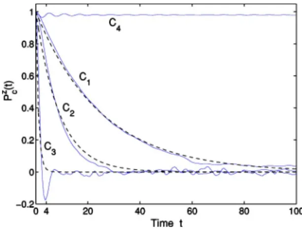
In Fig. 3 the time dependences of P_cz共t兲 for 2124 electrons in the open system [Fig. 2(a)] with Lso= 10, 6, and 2 are plotted by solid curves C1, C2, and C3. One can see that the relaxation time increases with Lso. These curves can be fitted by the well-known expression for the longitudinal DP relaxation19

PDP共t兲 = exp

冉

− 4tlm

L_so2

冊

, 共28兲 which is shown by the dashed curves in Fig. 3. This expres-sion was derived under the assumption of sufficiently large LsoⰇlm. For not so large Lsothe fitting is not good, as it can be seen for the curve C3 around its first drop at t = 4. In this

regime the spin rotates rather fast, so that most of the spins s_z共i兲共t兲 evolve to negative values before the electrons encoun-ter their first collisions with impurities. Therefore, P_cz共t兲 can evolve to a deep negative value within a short time interval. But later on P_cz共t兲 approaches to the asymptotic value P_cz= 0

(curve C3 in Fig. 3). These results from Monte Carlo simu-lations confirm the well-known DP relaxation in unbounded systems.

If electrons are confined inside the smooth circular dot

[Fig. 2(b)], the relaxation of Pc

z_{共t兲 is considerably}

sup-pressed, so that at large Lso the spin polarization remains close to 1 at large times, as the curve C4 in Fig. 3 demon-strates for the case of Lso= 10. At this regime, the suppression of relaxation takes place in all other quantum dots, like the circular dot with the rough boundary(curve C6), the triangu-lar dot(curve C7), and the Sinai billiard (curve C8) in Fig. 4. In all of these curves the P_cz共t兲 values fall into the range between 0.97 and 0.98 at large times up to t = 103_.

On the other hand, the spin polarization evolves very fast down to 0 if Lsois smaller than the dot size. The correspond-ing time dependence of P_cz共t兲 is similar to that shown in Fig.

FIG. 5. (Color online) Time dependence of P_cz共t兲 for Lso= 2 in the smooth circular dot(curve C₅), the circular dot with the rough boundary(curve C6), the triangular dot (curve C7), and the Sinai billiard(curve C₈).

FIG. 3. Solid curves C1, C2, and C3represent the time depen-dent polarization P_cz共t兲 for 2124 particles in an unbounded QW with

Lso= 10, 6, 2, and the mean free path lm= 1. The particles were

initially placed inside a circular area of the radius R = 1 and polar-ized in the z direction. The dashed curves depict the DP relaxation calculated from Eq.(28). For comparison, curve C₄shows P_cz共t兲 for 2124 particles confined inside a circular dot of the radius R = 1 and

L_so= 10.

FIG. 4.(Color online) Time dependence of Pc z_{共t兲 for L}

so= 10 in the smooth circular dot(curve C5), the circular dot with the rough boundary(curve C₆), the triangular dot (curve C₇), and the Sinai billiard(curve C8).

(7)

3(curve C₃), with a sharp drop at the beginning followed by oscillations around zero.

For an intermediate Lsothe spin relaxes according to dif-ferent scenarios, depending on the quantum dot geometry. As an example, Fig. 5 shows the function P_cz共t兲 for various dot geometries at Lso= 2. After a fast initial drop, the polarization further relaxes to 0 in the Sinai billiard(curve C8) and in the circular dot with the rough boundary(curve C6). However, in the smooth circular(curve C5) and triangular (curve C7) dots this function oscillates around a constant value at large times. It should be noted that in the former two examples the spin polarization relaxes to zero at much longer times than the DP relaxation time in the unbounded system(Fig. 3), although the mean elastic scattering length there is comparable to the dot size. The relaxation times for C₆ and C₈ in Fig. 5 in-crease rapidly with higher Lso. Thus, at Lso= 10 we could not detect any systematic decrease of the spin polarization in the Sinai billiard and rough circular dot, up to t = 103_{, which is} by an order of magnitude larger than the range plotted in Fig. 4.

An interesting feature of P_cz共t兲 in the regular systems, like the triangular and smooth circular dots, is the apparent oscil-lation of the polarization. It can be seen in Figs. 4 and 5, although the oscillations in the latter figure are more pro-found for the case of the circular dot, compared to almost vanishing ripples in the triangle. These oscillations do not disappear at large times and their amplitudes increase with the strength of SOI. We cannot say much about their nature. Probably, they are associated with the role of periodic trajec-tories in regular systems. A special study is required to un-derstand the origin and characteristics of these oscillations.

At long time the spin polarizations in both regular quan-tum dots(triangle and smooth circle) in Figs. 4 and 5 oscil-late around certain nonzero residual values. These residual polarizations P_czare Lsodependent, as plotted in Fig. 6 for the circular dot.

C. Spin evolution along individual trajectories The existence of the nonzero residual polarization in regu-lar quantum dots and long spin relaxation time in chaotic

systems are fundamentally distinct from the DP spin relax-ation in the boundless QW. Such a distinction is surprising, because at first sight the spin walks on the sphere in Fig. 1(c) should be randomized by scattering of particles from dot boundaries, similar to randomization by impurity scattering in unbounded systems. However, this simple point of view is wrong, because there is an important difference between the impurity scattering and the boundary scattering. For conve-nience, let us define the scattering with a direction change smaller than ␲/ 2 as a “forward” scattering and that larger than␲/ 2 as a “backward” scattering. If the particles are iso-tropically scattered by an impurity, half of them continue to move “forward.” However, if the particles are scattered by a smooth boundary, the particles with incident angles between −␲/ 4 to ␲/ 4 with respect to the boundary normal will be reflected “backward.” Since statistically more particles hit the boundary within this range of angles, the “backward” scattering prevails in DQ’s. This property of particle scatter-ing can also be extended to QD’s with rough boundaries. Further, according to Fig. 1, a “backward” particle motion is mapped onto a “backward” spin walk. Hence, if the spin moves away from the north pole in Fig. 1, after a boundary scattering the spin is more likely bounced back toward the north pole. Such a non-Markovian statistic of the spin walks gives a clue for understanding the numerical results in Sec. III B.

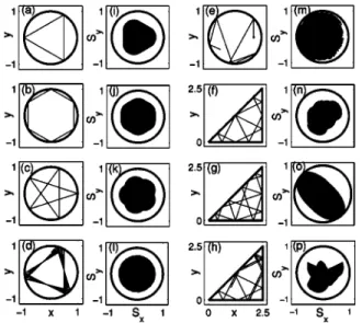
In order to make this argument more clear it is instructive to study in detail the spin evolution along a single trajectory. As described in Fig. 1, the spin motion on the unit sphere can be projected onto the sxsyplane. After a long time the spin

path on the sphere will cover a region and produce a certain pattern on the s_xs_yplane. In the circular dot this pattern looks rather ordered. If the electron moves along a triangular peri-odic trajectory[Fig. 7(a)], the pattern is a rounded triangle FIG. 7. Electron trajectories on the xy plane[(a)–(h)] and re-spective spin evolution patterns on the sxsy plane[(i)–(p)] for Lso = 5. (a), (b), and (c) periodic triangular, hexahedral, and starlike trajectories in the smooth circular dot.(d) A nonperiodic trajectory in the smooth circular dot.(e) A stochastic trajectory in the rough circular dot.(f) and (g) Two periodic trajectories in the triangular dot.(h) A nonperiodic trajectory in the triangular dot.

FIG. 6. The residual polarization P_czvs the spin rotation length

(8)

[Fig. 7(i)]. If the trajectories are hexahedral and starlike [Figs. 7(b) and 7(c)], the corresponding patterns are a

rounded hexagon and a rounded star[Figs. 7(j) and 7(k)]. If the trajectories are nonperiodic, e.g., Fig. 7(d), the pattern is a disc[Fig. 7(l)]. A common feature of these patterns is that they have the same size, which is less than 1 in the case of Lso= 5. These patterns are highly stable up to the observation time t = 104. It implies that the spin on the unit sphere cannot move far away from the north pole, so that s_z共i兲共t兲 cannot take negative values. Our analysis of various trajectories with various initial conditions has confirmed this general feature of the spin evolution in the circular dot. Hence, a nonzero P_cz in Fig. 6 at infinitely long time is obviously expected.

In the triangular dot, two periodic and one nonperiodic trajectories are shown in Figs. 7(f)–7(h). The corresponding spin patterns[Figs. 7(n)–7(p)] are less symmetric and have less predictable sizes than those in the circular dot. For the trajectory in Fig. 7(g) the pattern in Fig. 7(o) touches the circular border. Nevertheless, our investigation shows that the patterns of most other trajectories are quite stable up to the observation time 104_{and do not touch the border. On this} reason the spin polarization being averaged over trajectories is expected to relax to a positive residual value, although this value is smaller than that in the smooth circular dot.

In the circular dot with a rough boundary, the reflection angles are stochastic, as shown in Fig. 7(e). Within the ob-servation time t = 103 _{the corresponding spin pattern on the} sxsyplane has spread out to a much larger area [Fig. 7(m)]

than those in the smooth circular dot [Figs. 7(i)–7(l)]. Fur-thermore, the pattern in Fig. 7(m) is still expanding. The corresponding spin state on the 3D sphere can penetrate into the lower hemisphere after t = 103. However, it can return back to the north sphere again. Therefore, the z component of this spin state oscillates between negative and positive values. When averaged over many trajectories, such oscilla-tions sum up to a relaxation curve, similar to C₆ in Fig. 5.

In the Sinai billiard, the sxsypattern resembles that in the

rough circular dot. Consequently, the spin relaxation dynam-ics in both cases have similar characteristdynam-ics(curves C6and C8in Fig. 5).

A general trend seen from Fig. 7 is that the confinement of the particle motion in QD’s makes the spin to be also con-fined within the upper hemisphere, if Lso is larger than the size of the QD’s. For a smooth circular dot, this trend can be easily understood from the “backward” scattering effect de-scribed at the beginning of this subsection. Since all trajec-tories in this case have a simple geometry, one can easily see that particles are more frequently scattered from the bound-ary in a “backward” direction. But although this argument holds for general bounded systems, it is less evident for other QD’s besides the smooth circular dot. In a general case, the trend toward the spin confinement can be argued in a differ-ent way: As seen from Fig. 1, the projected spin path on the sxsyplane in Fig. 1(b) is more or less a rescaled curve of its

particle trajectory in Fig. 1(a). But in reality the mapping from a trajectory to the corresponding spin path is not simply a rescaling, because the spin rotations on the sphere are non-commutative. For example, a closed particle trajectory is in general mapped onto an open spin path. However, if Lso is large, the spin path is restricted to a small part of the sphere.

According to Eqs.(21) and (22), a closed particle trajectory produces an open spin path of the linear size⬃1/Lso, while the distance between the initial and the end points of the path is only ⬃1/L_so2. The mapping between the trajectories and the spin paths is then similar to a mapping between two Euclidean spaces. Therefore, with the accuracy 1 / L_so2, the spin paths are the rescaled particle trajectories and those paths are confined because the particle trajectories are con-fined. It should be noted that such a tendency for the spin confinement turns out to be strong even for not so large Lso, as one can see from the spin dynamics shown in Fig. 5 for Lso= 2.

The above argument about the spin confinement does not take into account a long time evolution. Even at large Lso, small corrections due to noncommutativity of spin walks will accumulate in time. As a result, the spin can slowly drift toward the lower hemisphere. The expanding pattern in Fig. 7(m) of the rough circular dot is an example of such a long time behavior. However, in contrast to that unstable pattern, the patterns from regular systems [Figs. 7(i)–7(p) besides 7(m)] remain stable in time. This difference between the single trajectories of random and regular systems is consis-tent with the spin relaxation curves shown in Fig. 5.

Such a distinction between regular and chaotic systems follows from fundamental properties of regular and chaotic systems. It can be understood from consideration of periodic orbits. After a particle runs along a periodic orbit␥and com-pletes a period, its initial spin state␹will evolve to U_␥␹with U_␥= exp关−i⍀R␴兴, which represents a rotation around the axis R through the angle 2⍀. Both R and ⍀ are determined entirely by the geometry of␥ and by the value of Lso. After the particle repeats w periods, all spin positions共U_␥兲w␹, cor-responding to the end points of all periods w = 1 , 2 , . . ., are located on a closed circle. This circle can be obtained by rotating the north pole around R, if the initial␹is related to the spin polarized in the north pole direction. The other points on the periodic orbit are mapped onto spin states around this circle. Taking many periodic orbits into account, one obtains a set of different axes R and consequently a set of circles passing through the north pole. Hence, when aver-aged over all periodic orbits, spin spends more time in the upper hemisphere. This means that at least the family of the periodic orbits contributes to a nonzero residual polarization. How significant is this contribution to the whole residual value depends on the amount of the periodic orbits in a sys-tem, which is quite different in regular and chaotic systems. In a regular system the family of periodic orbits has a finitely positive measure and a bundle of adjacent nearly periodic orbits. These adjacent trajectories behave like periodic orbits if the time is not too large, because their linear deviation in time from the periodic orbits is small. On the contrary, the periodic orbits in chaotic systems are of zero measure.20 Fur-thermore, their adjacent trajectories deviate from them expo-nentially fast. Therefore, with increasing time, the weight of the periodic orbits and their adjacent trajectories becomes exponentially small in chaotic systems, while it is a nonzero value in regular systems. Hence, as long as we consider only periodic orbits, the residual spin polarization has to be a positive number for regular systems and zero for chaotic sys-tems.

(9)

The individual trajectory study in a larger time scale car-ried out in this section helps us to understand some of the results in Sec. III B. However, although the indication of the nonzero residual polarization P_cz from Figs. 3–6 is strong, one might still suspect that P_cz will decay to zero within a much larger time scale, since the numerical simulations in all these figures are truncated at a finite time. This suspicion can be tested by calculating the exact spin polarization quantum mechanically, if the analytical solutions of the Schrödinger equation are available in the systems. Indeed, this exact re-sidual polarization value is nonzero in the smooth circular dot, as shown in the next section.

IV. QUANTUM MECHANICAL POLARIZATION IN THE CIRCULAR QUANTUM DOT

Due to the time reversal symmetry, the quantized energy levels En of the Hamiltonian H in Eq.(1) are, at least,

two-fold degenerate with the corresponding spinor eigenfunctions ␸na, where a苸兵±其 is the degeneracy index. In the basis of

these states a normalized wave function ␺共r,t兲 can be ex-panded as

␺共r,t兲 =

兺

na

cna␸na共r兲e−iEnt/ប, 共29兲

with the coefficient

cna=

冕

␸na

†_共r兲_␺_共r兲d2_r. _共30兲 The expression of ␺共r,t兲 in Eq. (29) differs from Eq. (3) only by the degeneracy index a, which is explicitly written here for convenience of our further analysis. Taking the no-tation

␺na共r,t兲 = cna␸na共r兲e−iEnt/ប, 共31兲

and␺na共r兲=␺na共r,0兲, the z component of the quantum

me-chanical polarization in Eq.(5) can be expressed as

Pz共t兲 = 具␺共r,t兲兩␴z兩␺共r,t兲典=

兺

nab

冕

␺na †_共r兲 ␴z_␺ nb共r兲d2r +

兺

n⫽m,ab

冕

␺na †_共r兲_␴z_␺

mb共r兲ei共En−Em兲t/បd2r. 共32兲

The first sum in this equation is time independent, while the second sum oscillates in time, so that its average over a sufficiently long time interval turns to zero. It is interesting to find out whether the former term coincides with the re-sidual polarization in Fig. 6. Such a coincidence is not evi-dent because the time depenevi-dent sum can give rise to large variations of Pz共t兲 after long time t. Moreover, the semiclas-sical theory employed in the previous section cannot be valid for times larger than the mean distance between energy lev-els near the Fermi energy. We can check such a coincidence at least for the simple case of a circular dot with the smooth boundary, by calculating the residual polarization

Pz=

兺

naa⬘

冕

␺na

† _共r兲_␴z_␺

na⬘共r兲d2r, 共33兲

because the analytic solution of the Schrödinger equation with the arbitrarily strong Rashba interaction is available.21 In this section only the key steps of the calculation are pre-sented, while the calculation in detail is shown in the Appen-dix.

Let us consider a circular quantum dot of radius R with the confining potential

V共␳兲 =

再

0 for 0艋␳艋 R

1

0

冊

e

ikr _共42兲

as the initial state. After inserting␸n+共r兲 from Eq. (35) and

␸n−共r兲 from Eq. (36) together with Eq. (31) into Eq. (33) and

averaging over directions of the vector k we obtain Pz= 2␲

兺

n

共兩cn+兩2−兩cn−兩2兲共Fn− Gn兲, 共43兲

(10)

Fn= d2关a␯ 2 I_␯共1兲− 2a_␯I_␯共2兲+ I_␯共3兲兴 Gn= d2关a␯ 2 I_␯+1共1兲 + 2a_␯I_␯+1共2兲 + I_␯+1共3兲兴, 共44兲 where the coefficients I_␯共1兲, I_␯共2兲, and I_␯共3兲are presented in Eq.

(A18). The coefficients兩cn±兩2in Eq.(43) can be written as 兩cn+兩2= 4␲2d2共− a␯I_␯共4兲+ I_␯共5兲兲2

兩cn−兩2= 4␲2d2共a␯I_␯+1共4兲 + I_␯+1共5兲兲2, 共45兲

with the coefficients I_␯共4兲and I_␯共5兲given by Eq.(A21). Using the dimensionless units, one has the radius R = 1, the cou-pling constant b = 2 / Lso, and the wave-number k = 2␲R /␭, where␭ is the electron wavelength. Hence the semiclassical range of parameters corresponds to kⰇ1.

The residual polarization calculated from Eq. (43) is shown in Fig. 8. The Pzcurves for k = 20, 30, and 40 are very close to each other and merge into the dashed curve. This curve coincides with the residual polarization obtained from the semiclassical simulations in the previous section(Fig. 6). For k = 5, 1, and 0.1, the curves are plotted in the dotted, solid, and dash-dotted curves, respectively. All the curves, as expected, have the common asymptotic value 1 in the case of the weak spin-orbit coupling Lso→⬁. In the opposite limit, L_so→0, the behavior of Pz _{is nonanalytic and not much}

re-vealing. The strong oscillations in this limit increase with smaller wave numbers and signal about the appearance of large quantum beats in Pz_{共t兲. This regime of L}

sois not inter-esting from the practical point of view because it implies unphysically large values of␣_R for the typical dot radius R = 500 nm. In the practically important regime of Lso艌1 we note an apparent dependence of Pz on k at k艋5. This is a quantum effect which is not observed in our semiclassical simulations. In semiclassics the particle velocity determines the speed with which Pz_{共t兲 approaches to the residual value}

Pz, but not this value itself.

V. DISCUSSION

Summarizing the above results of the semiclassical Monte Carlo simulations and quantum mechanical calculations we can draw the following picture of the spin evolution in semi-classical quantum dots. In the dots with regular semi-classical dy-namics the spin polarization does not decay to zero at long time and its residual value coincides with the quantum me-chanical spin polarization averaged over an infinitely long time interval. At least, we were able to check such a coinci-dence for the circular dot. On the other hand, in dots with chaotic or random dynamics the spin polarization relaxes to zero with the relaxation time much larger than the DP relax-ation time in unbounded quantum wells. Such a decay down to zero cannot be understood from the general quantum me-chanical expression in Eq.(32) , because it implies that the average of Pz_{共t兲 over an asymptotically long time interval is}

zero. However, Eq.(32) predicts that this average is given by the first term in Eq.(32), which is nonzero in general. Obvi-ously, this contradiction is associated with quantum mechani-cal effects, which indicates that the semiclassimechani-cal approxima-tion is insufficient for analysis of the long time polarizaapproxima-tion evolution. Indeed, studies of electron transport in chaotic and disordered QD’s have shown that the quasiclassical method is valid only at sufficiently short times.22–25 _{An important} crossover time is the Ehrenfest time TE. This time is

con-trolled by the Lyapunov exponent describing the divergence of close trajectories in chaotic systems. Within T_E two tra-jectories initially located at a distance of the order of the de Broglie wavelength will diverge up to a distance comparable to the size of the QD. The importance of quantum effects at times larger than T_E has been demonstrated for Andreev bil-liards in Refs. 22–24. Another characteristic time is given by T_⌬=ប/⌬, where ⌬ is the mean distance between energy lev-els in the QD. In disordered mesoscopic systems the statis-tics of their energy spectrum together with the weak local-ization effects give rise to the so-called quantum dynamical echo at t⬎T_⌬. This phenomenon was investigated for the time evolution of the electron density in a noninteracting electron system.25_{It was found that due to the quantum} ef-fects the density profile at large time is inhomogeneous throughout the QD and preserves the memory about the ini-tial density distribution up to the dephasing time. One can expect a similar memory effect for the spin polarization. At least for an unbounded 2D gas the weak localization correc-tion to the DP relaxacorrec-tion was shown to produce a nonexpo-nential 1 / t tail in the spin polarization evolution at large times.26 _{This problem is outside the method of the present} work and needs further study.

The predicted spin evolution can be measured experimen-tally. For an InAs dot doped up to 1011_cm−2_{, the time unit in} Figs. 3–5 is about 1 ps if the dot size is L = 0.5␮m. Hence, the spin polarization saturates to its residual value during first 20 ps and for Lso= 1␮m the difference in the long time evolution between chaotic and regular dots can be observed in the nanosecond range. In order to suppress all inelastic spin relaxation mechanisms,3–6 the measurement must be done at sufficiently low temperatures. The Rashba spin-orbit interaction can be strong in InAs based heterostructures, with Lsodown to several hundreds nm. Moreover, it can be tuned FIG. 8. (Color online) The residual spin polarization Pzvs Lso

with k = 20, 30, 40, (dashed), k=5 (dotted), k=1 (solid), and k = 0.1(dash-dotted). The dashed curve coincides with the curve from

(11)

in a wide interval by varying the gate voltage.12

In conclusion, we performed path integral semiclassical simulations of spin evolution controlled by the Rashba spin-orbit interaction in quantum dots of various shapes. Our cal-culations revealed that the spin polarization dynamics in QD’s is quite different from the D’yakonov-Perel’ spin relax-ation in bulk 2D systems. Such a distinction is not expected from the simple picture of the spin random walk, in particu-lar when the rate of electron elastic scattering on impurities in bulk is equal to the mean frequency of electron scattering from the dot boundaries. We have also found an important distinction between long time spin evolutions in classically chaotic and regular systems. In the former case the spin po-larization relaxes to zero within relaxation time much larger than the DP relaxation, while in the latter case it evolves to a time independent residual value. This value decreases with the stronger spin orbit interaction. We also analyzed the gen-eral quantum mechanical expression for the time dependent spin polarization. Using the exact solutions of the Schrödinger equation with Rashba SOI for a circular dot, we calculated the average of the spin polarization over an infi-nitely long time interval and compared the result with the residual polarization from the Monte Carlo simulations. We found that the residual values from these two approaches coincide, which confirms the results from the semiclassical simulations. On this basis, we conjecture that the nonzero residual value is a general property of regular systems. On the other hand, the spin relaxation down to zero in the Sinai billiard and circular dot with the rough boundary contradicts what has to be expected from quantum mechanics. The long time memory due to the mesoscopic spin echo is assumed to be responsible for this contradiction.

ACKNOWLEDGMENTS

This work was supported by RFBR No. 03-02-17452 and the Swedish Royal Academy of Science; A.G.M. edges the hospitality of NCTS in Taiwan. C.-H.C. acknowl-edges the hospitality of Lund University in Sweden and the Science Institute in the University of Iceland.

APPENDIX

This Appendix demonstrates a quantum mechanical cal-culation of the residual polarization Pz, as it is defined in Eq.

(33). The calculation of the exact eigenfunctions of the

Hamiltonian in Eq.(1) for the circular quantum dot can be found in Ref. 21, which is summarized in the following Eqs.

(A1)–(A5).

In order to calculate the residual polarization (33), the wave-function␺na共r兲 is expanded in the basis of the

eigen-functions given by Eqs. (35) and (36). We note that for a symmetric presentation, the functions f_␯and g_␯ have differ-ent definitions from those in Ref. 21. Inserting Eqs.(35) and

(36) into the corresponding Schrödinger equation we obtain

the equation for f_␯ and g_␯ in terms of the dimensionless parameters␰,␧, and b defined in the previous section

关䉭_␯+␧兴f_␯共␰兲 − b ⵜ₋_共␯+1兲g_␯+1共␰兲 = 0,

关䉭_␯+1+␧兴g_␯+1共␰兲 − b ⵜ₊_␯ f_␯共␰兲 = 0, 共A1兲 with the Laplacian

䉭␯= 1 ␰ d d␰

冉

␰ d d␰

冊

− ␯2 ␰2 共A2兲

and the nabla operator

ⵜ±␯= ±

冉

d d␰

冊

−

␯

␰. 共A3兲

The solutions关f_␯共␰兲,g_␯共␰兲兴 of these equations are

冉

f_␯共␰兲 g_␯共␰兲

冊

= d

冉

− a_␯J_␯共k+␰兲 + J␯共k−␰兲 a_␯−1J_␯共k+␰兲 + J␯共k−␰兲

冊

, 共A4兲

with the normalization constant d, the factors a_␯given by Eq.

(38), and the wave-vectors k± from Eq. (39). These wave vectors obey the relations

k+k−=␧, k+− k−= − b,

and k++ k−=

冑

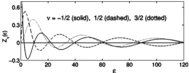
b2+ 4␧. 共A5兲 The quantized dimensionless energies ␧ are determined by the zeros of the function in Eq.(41) . This function stems from the determinant of the equation system in Eq.(A1) with the boundary conditions f_␯共␰兲=g_␯共␰兲=0 at␰= 1. Given a cou-pling constant b, the nth quantized value ␧n with n

= n共␭,␮兲 is determined by the␮th zero of Z_␯共␧兲, where␯and

␭ are related by Eq. (40). The allowed wave-numbers k±are given by Eq. (39) with ␧=␧_n. They correspond to the two degenerate eigenstates of the nth energy level. The first root of the function Z_␯共␧兲 is zero for ␯= 1 / 2 , 3 / 2 , . . ., and is a positive value for␯= −1 / 2 (see Fig. 9). The larger the value of b, the larger the second root of Z_␯共␧兲.

Substituting the wave functions in Eqs.(35) and (36) into Eq.(33) we obtain the residual polarization in the form

Pz=

兺

n

冕

0 1

冕

0 2␲ 关共兩cn+兩2−兩cn−兩2兲关f_␯ 2_共 ␰兲 − g_␯+12 _共 ␰兲兴 + 2c_n+* cn−f␯共␰兲g␯+1共␰兲e−i共2␯+1兲␾ + 2c_n−* c_n+f_␯共␰兲g_␯+1共␰兲ei共2␯+1兲␾兴 d␾ ␰d␰. 共A6兲 For the initial wave function given by Eq.(42) , the con-stants cn+can be expressed as

FIG. 9. The function Z_␯共␧兲 for ␯=−1/2, 1/2, and 3/2. This function is singular at␧=0 for␯=−1/2.

(12)

cn+=

冕

冕

0 1 ei关k␰ cos共␾兲−␯␾兴f_␯共␰兲␰d␰d␾. 共A8兲 Substituting t =␾+␲/ 2 and m =␯ into the integral represen-tation of the Bessel function,27

Jm共z兲 = 1 2␲

冕

₋_␲ ␲ ei关z sin共t兲−mt兴dt, 共A9兲 we obtain 2␲ei␯␲/2J_␯共z兲 =

冕

0 2␲ ei关z cos共␾兲−␯␾兴d␾. 共A10兲 By using this identity, Eq.(A8) can be written as

cn+= 2␲ei␯共␲/2−␪兲

冕

0 1

J_␯共k␰兲f_␯共␰兲␰d␰. 共A11兲 By analogy, one has

cn−= 2␲ei共␯+1兲共␲/2−␪兲

冕

0 1

J_␯+1共k␰兲g_␯+1共␰兲␰d␰. 共A12兲 After integrating Eq.(A6) over␾and the direction␪of k

[integration over␪is similar to that over␪kin Eq.(20) ], the

0 l ␰J_␯共␭␰兲J_␯共␬ ␰兲d␰ =l关␬J␯共␭ l兲J␯+1共␬l兲 − ␭J␯共␬l兲J␯+1共␭ l兲兴 ␬2₋_␭2 . 共A15兲

Consequently, the integrals in Eq.(A13) can be written in the closed form Fn= d2关 a␯ 2 I_␯共1兲− 2a_␯I_␯共2兲+ I_␯共3兲兴, 共A16兲 Gn= d2关a_␯ 2 I_␯+1共1兲 + 2a_␯I_␯+1共2兲 + I_␯+1共3兲兴, 共A17兲 with I_␯共1兲=J␯共k+兲 2_{+ J} ␯+1共k+兲 2 2 − ␯J_␯共k₊兲J_␯+1共k₊兲 k+ , I_␯共2兲=k−J␯共k+兲J␯+1共k−兲 − k+J␯共k−兲J␯+1共k+兲 k₋2− k₊2 , I_␯共3兲=J␯共k−兲 2_{+ J} ␯+1共k−兲2 2 − ␯J_␯共k−兲J␯+1共k−兲 k− . 共A18兲

By analogy, calculating the integrals in Eqs. (A11) and

(A12) we obtain 兩cn+兩2= 4␲2d2共− a␯I_␯共4兲+ I_␯共5兲兲2, 共A19兲 兩cn−兩2= 4␲2d2共a␯ I_␯+1共4兲 + I_␯+1共5兲兲2, 共A20兲 with I_␯共4兲=k+J␯共k兲J␯+1共k+兲 − kJ␯共k+兲J␯+1共k兲 k+ 2 − k2 , I_␯共5兲=k−J␯共k兲J␯+1共k−兲 − kJ␯共k−兲J␯+1共k兲 k₋2− k2 . 共A21兲

For small b the spin polarization approaches to Pz_{= 1, as it}

must be in the absence of the spin-orbit interaction. It fol-lows from the relation k−− k+= b⬇0 in Eq. (A5), which re-sults in f_␯共␰兲⬇0, according to the definition in Eq. (A4). Hence, the two quantities兩cn+兩 and Fn, which contain f␯共␰兲,

vanish in Pz_{. Therefore, the sums in the numerator and}

de-nominator of Pz _{become the same, which gives rise to P}z

= 1.

For large b, we have Pz→0, which is due to the large difference between k+and k−, namely, k−− k+= bⰇ1. Accord-ing to the asymptotic behavior28

J_␯共x兲 =