Belle II 實驗第一級觸發器中二維軌跡探測器之實現

(1)

..

國立臺灣大學理學院物理學系碩士論文

Department of Physics College of Science

National Taiwan University Master Thesis

Belle II 實驗第一級觸發器中二維軌跡探測器之實現 Implementing the 2D track reconstruction for the

Level 1 trigger of the Belle II experiment

盛子安 Tzu-An Sheng

指導教授：張寶棣博士 Advisor: Paoti Chang, Ph.D.

中華民國 107 年 7 月

July, 2018

(2)

..

(3)

..

誌謝

碩士班的光陰，三分積澱在這卷論文的算式圖表中，剩下的七分化作煙塵，隨風搖落在經途草木之下。這些無緣成為論文題目的研究歷練，縱然有欠完整，也依舊滋養了百木；儘管遠僻，也絕不失蔥鬱。但願有朝一日，我會慶幸曾在這片森林裡踟躕過。

在這裡特別向這幾條研究的「歧途」上，提攜我的貴人們致謝。感謝張寶棣、徐靜戈、王名儒三位老師對我物理分析技巧的琢磨與指導，

也感謝李彥頡老師在我們合作的研究中，給予我熱情與鼓勵。感謝賴昀樅悉心的教學與敦促，更感謝曾衍銘對我傾囊相授研究經驗與心法。

感謝黃坤賢活絡了學生之間的交流討論，也感謝張祐豪、張硯詠帶給實驗室無盡的精神食糧。感謝柯尹拉 (Suman Koirala) 數度肯定我另闢蹊徑的分析程式架構，也感謝裴思達 (Stathes Paganis) 老師向我分享高能物理實驗的樂趣。感謝稻見武夫老師提供我在研究之外，能站在講台上與學生們切磋習題的經驗，也感謝陳昱潭屢次在我困於研究生活的水火中時遞出的關懷。感謝劉建宏與趙元對我在管理組內伺服器與在台大架設測試站時大力相助，也感謝黃子娟、周建宏對我實驗上的的諸多幫助與指導。限於篇幅，感謝所有和我一起在碩士班修課、談天與苦惱的好友。

最後深深感謝父母在我稍長的求學期間，對我的支持與縱容。

(4)

..

(5)

..

Acknowledgements

I would like to thank my advisor, Prof. Paoti Chang, who taught me about particle physics and strives for funding. I am also grateful to Dr. Jing-Ge Shiu for his great mentoring.

I am indebted to Dr. Sara Pohl, who raised the theoretical performance of the 2D tracker, helped me with the code, and never ceases to amaze me with her thoughtfulness in this research. I also appre- ciate Dr. Yun-Tsung Lai’s perseverance to smooth the data transmission. Thank Dr. Yoshihito Iwasaki for his good leadership. Thank Dr. Hideyuki Nakazawa for the help with the data taking and his kind support during my stay at KEK. Thank Dr. Jae-Bak Kim for all his in- spiring ideas. Thank Prof. Jeri M.C. Chang for bringing the research topic to me.

Thank Shiu-san, Nakazawa-san and Jeﬀery Chiang for their pa- tience as editors and readers of the draft.

(6)

..

(7)

..

摘要

位處日本筑波的 B 介子工廠：KEKB 正負電子加速器與 Belle 實驗，

透過研究 B 介子衰變中，弱作用之電荷對稱宇稱破壞的現象，奠定了小林──益川理論的實驗基礎，並且促成 2008 年的諾貝爾物理獎。為了從稀有衰變中探究粒子物理標準模型以外的新物理，此工廠正升級為 SuperKEKB 加速器與 Belle II 實驗，將加速器瞬時亮度提升至 8 × 10³⁵cm⁻²s⁻¹（原先的 40 倍）。然而在 Belle II 偵測器中，資料擷取的速率上限僅為每秒 3 萬次，並不能紀錄新亮度之下所有的對撞事例。實際上，具研究價值的Υ 介子、B 介子及τ 子等事例僅佔所有對撞事件的數個百分比。另外還有許多偵測器反應並非對撞事件，而是源自加速器中帶電粒子簇的散射、同步輻射、或是粒子與真空管線中殘餘空氣分子碰撞等背景雜訊。為了在資料擷取的速限之下盡可能紀錄所有珍貴的事例，Belle II 實驗勢必得仰賴一套基於硬體的即時觸發系統，提供高效率、低延遲、無死區時間的事例判別，使資料擷取系統得以忽略背景事例，不至受到掣肘。

由於多數背景事例不會在碰撞點附近產生具高橫向動量的帶電粒子，這樣的粒子便成為判別背景事例的關鍵。因此，Belle II 實驗將帶電粒子軌跡觸發器重新改造，以因應加速器亮度提升。在高能加速器實驗中，透過辨認帶電粒子通過偵測器時，在數十處感應線留下的電流訊號，我們得以重建帶電粒子的空間軌跡。由於偵測器內通有縱向磁場，我們亦可藉螺旋軌跡推知粒子的動量。掌握帶電粒子的數量、動量等資訊，並輔以量能器能量團與帶電粒子軌跡的空間對應關係，便能輕易地區分目標事例與背景事例的差別。

(8)

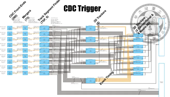
.. 帶電粒子留下的電流訊號經過數位化後成為擊打訊號，輸入至軌跡觸發器。軌跡觸發器首先將偵測器中相鄰的擊打訊號組成區段擊打訊號。每個帶電粒子軌跡由最多 9 層的區段擊打訊號所組成，其中 5 層包含了三維的粒子螺旋軌跡在偵測器橫段面上所投影出的二維圓弧軌跡訊號。這 5 層訊號的幾合位置透過共形變換以及霍夫變換後，在軌跡參數空間中形成許多三角函數曲線。藉由尋找參數空間中 4 條以上來自不同層的曲線交點，可知幾何空間中四層以上共圓弧的區段擊打訊號，與該圓弧所對應的粒子橫向動量之大小及方向。將橫向動量與剩餘四層包含粒子螺旋軌跡縱向資訊的區段擊打訊號結合後，即可推知完整的三維軌跡。

前述尋找區段擊打訊號、尋找二維軌跡及尋找三維軌跡的步驟皆由各別的硬體模組所實現。另外，軌跡觸發器還包含了整合最前端感應線擊打訊號的模組。各模組之間由光纖傳輸連接。本論文著重於將上述由二維區段擊打訊號尋找二維軌跡的演算法，以現場可程式化邏輯閘陣列實現。實現後的邏輯延遲為 11 個時脈周期（相當於 350 奈秒，

不包含傳輸所需的延遲）。透過測量宇宙射線事例，並與更精密的軟體軌跡重建方法比較後，我們推估對於所有橫向動量在0.5 GeV以上、與碰撞點徑向距離小於 1 公分、含有 4 個以上區段擊打訊號、並且不受前端模組錯誤影響的所有軌跡，二維軌跡尋找效率在一個標準差之下的信心區間完全落在 98% 以上。

本論文同時紀錄了二維軌跡擬合的實現方法。這個方法利用軌跡偵測器中由高能帶電粒子碰撞氣體分子游離出的電子，以及由該電子游離出的次級電子在電場中的的飄移速度，通過測量飄移時間，推算出更精確的軌跡區段擊打位置，並且以最小平方法擬合得出更精密的二維軌跡。由於這個步驟將會併至更後端的三維軌跡擬合模組中實現，

並且包含大量需藉由查表實現的運算步驟，因此在不喪失計算精確度的前提下降低記憶體用量便成為最大的挑戰。我們發展了複和式的查表方法，並利用三角函數的對稱性減低記憶體用量。另外，本論文也包含數項對建立光纖傳輸資料流穩定性的改善。尤其透過以特定時間

(9)

.. 間隔重置位於晶片同一側的光纖收發器，我們得以在更高的傳輸速率下提升建立傳輸資料流的穩定性。

關鍵字： Belle II 實驗；模式辨認；粒子軌跡；CP 破壞；觸發器；現場可程式化邏輯閘陣列

(10)

..

(11)

..

Abstract

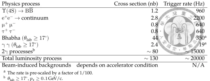
The Belle experiment at the KEKB collider in Tsukuba, Japan is a B meson factory designed to operate at a center-of-mass energy of 10.58 GeV, the mass value of Υ(4S). It is undergoing an upgrade that will boost its instantaneous luminosity to 8 × 10³⁵cm⁻²s⁻¹ (40 times higher than before), whereas the maximum acceptable event rate for the data acquisition system is only 30 kHz. Most of the detector re- sponses arise from the scattered particles with other particles in the accelerated bunch, or with the residual gas molecules in the vacuum beam pipe. Furthermore, only a few percent of the total number of e⁺-e⁻ collisions correspond to Υ, B or τ events. The rest are consid- ered backgrounds and must be either suppressed or prescaled in real time without losing too many signal events. To achieve this goal, a hardware-based online trigger system with good background suppression, high eﬃciency, low latency and no dead time is indispensable.

In experimental particle physics, tracking refers to the pattern recog- nition process that searches for the trajectories of charged particles by analyzing the traces they leave on the detector. Once the trajectory, or the track, is reconstructed, the momentum and the charge is also determined. High-precision tracking provides crucial information for telling signals from backgrounds, since most background events don’t produce charged particles with enough transverse momenta near the collision point. As a result, the track trigger in Belle II is redesigned

(12)

.. to accommodate the dramatic increase of luminosity and background rate.

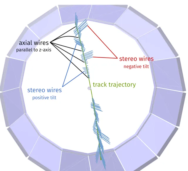
The track trigger starts from relating adjacent wire hits in space and in time from a drift chamber, grouping them into maximally 9 segments of a track. Out of the 9 segment hits, 5 are groups of sense wires parallel to the beam axis, and thus their positions contain information of the track projected onto the 2-dimensional plane perpendicular to the beam axis. The track trigger then detects the coincidence of several axial track segments by transforming their radial and angular positions to a parameter space with a conformal map followed by a Hough map, and looking for their intersections there. Each segment in one layer of the detector cylinder contributing to the track is extracted. Af- terwards, it ﬁts these positions with the drift length, and reconstructs the track’s projection in the plane perpendicular to the beam axis. Fi- nally, by combining the 2D track information with the remaining track segments which contains the information of longitudinal position, the vertex position along the beam axis is reconstructed. Each of these steps is a separate module in the track trigger system. This thesis fo- cuses on implementing the steps of ﬁnding and reconstructing the 2D track using an algorithm developed by our collaborator.

The 2D tracker module is implemented on 4 printed circuit boards with field programmable gate array (FPGA) and 10 Gbps optical I/O connection to both upstream and downstream modules. It has a latency of 11 data clocks (352 ns) excluding the transmission time. The lower bound of the 1-𝜎 confidence interval of its tracking efficiency is measured to be more than 98% for cosmic ray tracks with radial im- pact parameters smaller than 1 cm, 𝑝_t > 0.5 GeV, with at least 4 track segment hits, and coming from regions with expected track segment finding efficiency.

(13)

.. This thesis also outlines the implementation of the 2D fitter, which involves fitting an arc to the positions of the axial track segment hits corrected by their drift lengths. As the fitting contains many fixed- point arithmetic operations implemented as look-up tables, it is crucial to reduce the usage of the block RAM while maintaining similar arithmetic precision. Composite look-up tables, which increase the precision in the worst-performing part of the arithmetic function’s range by sacrificing the unnecessary precision in other parts, are developed to meet the requirement. Lastly, several improvements are made to stabilize the buildup process of the optical transmission data flow. In particular, an automatic way to reset different optical transceivers on the same side of the die, separated with an adjustable time interval, is tested to make the buildup more stable at the full 10 Gbps lane rate.

Keywords: Belle II; tracking; CP violation; trigger; FPGA

(14)

..

(15)

..

List of Figures

1.1 He/He ﬂux ratio. . . 3

1.2 The global CKM ﬁt in the ̄𝜌- ̄𝜂 plane . . . 19

1.3 Box diagrams of the B⁰self interaction . . . 20

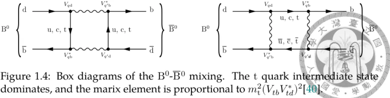
1.4 Box diagrams of the B⁰-B⁰mixing . . . 21

1.5 Feynman diagrams for B → Kπ, ππ . . . 27

1.6 Penguin contribution to B → ϕK . . . 31

1.7 The sin(2𝛽) values for decay modes related to b → s penguins . . . 32

1.8 Cross section of e⁺e⁻→ hadrons . . . 33

1.9 Background-subtracted Δt distributions and asymmetries . . . 33

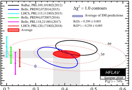
1.10 Current status of 𝑅_Dand 𝑅_D^∗ measurements . . . 35

1.11 The 𝑃₅^′ angular observable in bins of 𝑞² from LHCb Run 1 data . . . 37

1.12 Belle II detector . . . 39

2.1 Phase space plots of the beam particle . . . 47

2.2 Lattice design of the arc cell . . . 48

2.3 The SuperKEKB accelerator . . . 49

2.4 Schematic drawing around the positron target . . . 50

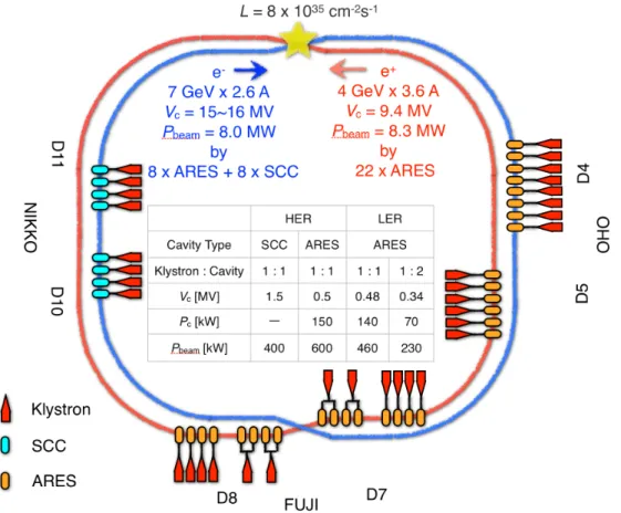
2.5 RF system in the main ring required to produce the ultimate luminosity . . . 51

2.6 Beam size near the collision point . . . 53

2.7 Crossing angle at SuperKEKB . . . 53

2.8 Horizontal and vertical collimators at SuperKEKB . . . 54

2.9 Scaler rates as a function of time after injection . . . 55

(22)

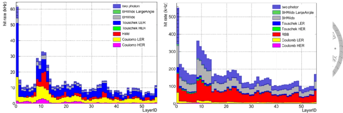
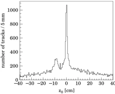
.. 2.10 Simulated background CDC wire hit rate . . . 57 2.11 Bunches in the storage rings of SuperKEKB . . . 57 2.12 Overview of the Belle II data acquisition system . . . 58 2.13 The Level 1 trigger system . . . 63 2.14 𝑧-vertex distribution of the tracks in Belle random trigger events . . 63 2.15 CDC in the Belle II and the Belle detector . . . 65 2.16 Wire configuration in the CDC . . . 66 2.17 Measured drift time v.s. drift length in the CDC . . . 66 2.18 3D view of the CDC wires related to a track . . . 67 2.19 CDC sub-trigger system . . . 68 2.20 A simulated event with background hits in the Central Drift Chamber 71 3.1 Transformation from the geometrical space to the parameter space 75 3.2 Conformal map . . . 75 3.3 The curves in the parameter space . . . 77 3.4 Voting in the accumulator space. . . 77 3.5 Tracking efficiency depending on 𝑝_tand number of TS hits . . . 78 3.6 Connected and disconnected cells. . . 79 3.7 Disconnected squares . . . 80 3.8 Clustering with the seed square . . . 80 3.9 The relation used in the 2D fitter . . . 83 4.1 The main boad of UT3 . . . 90 4.2 Acceptance range of the first 2D tracker . . . 93 4.3 Bit map of the 2D tracker input from Track Segment Finder . . . . 95 4.4 Bit map of the 2D tracker output . . . 97 4.5 Timing clones due to persistence and a trigger threshold of 4 TS hit 100 4.6 Logic diagram of the voting process . . . 102 4.7 Clustering of the squares in a block . . . 103 4.8 Logic diagram of finding the upper-right corner cell . . . 105

(23)

.. 4.9 Priority of choosing the corner square. Smaller numbers take prece- dence. . . 105 4.10 Decomposition of the cluster center . . . 106 4.11 Technology schematic diagram of the TS linking process using 2

clock cycles. . . 109 4.12 Technology schematic diagram of the TS linking process using only

1 clock cycle . . . 109 4.13 Persistence suppression . . . 110 4.14 Rules regarding whether to send new output . . . 110 4.15 Pipeline stages of the 2D tracker . . . 112 4.16 Schematic of the 2D fitter . . . 116 4.17 (Continued from Fig. 4.16) Schematic of the 2D fitter. . . 117 4.18 LUT function for tan⁻¹𝑥 . . . 118 4.19 Composite LUT for tan⁻¹𝑥. . . 119 4.20 Composite LUT made of 2 single LUTs . . . 119 4.21 Numerical error of tan⁻¹𝑥 with single and composite LUT . . . 120 4.22 The LUT function for cos 𝑥 . . . 121 4.23 The LUT function for tan⁻¹𝑥 . . . 121 4.24 Numerical error of the azimuthal angle to the Hough circle center 122 4.25 Numerical error of the transverse momentum . . . 123 4.26 RTL schematic of the logic in Fig. 4.8. . . 126 4.27 Technology schematic diagram of the logic in Fig. 4.8. . . 127 5.1 Track finding efficiency measured on single track events . . . 131 5.2 Track parameter resolution for two-track events . . . 132 5.3 Waveform of HDL simulation with SL-shifted hits as input . . . 133 5.4 Waveform of HDL simulation with TS-shifted hits as input . . . 133 5.5 TS acceptance of the 2D tracker with partial hit map input . . . 135 5.6 A single-track cosmic ray event . . . 136 5.7 Another single-track cosmic ray event . . . 137

(24)

.. 5.8 A multi-track cosmic ray event from a single source . . . 138 5.9 Waveform diagram of the event in Figure 5.8. . . 139 5.10 Another multi-track cosmic ray event from a single source . . . 139 5.11 Yet another multi-track cosmic ray event from a single source . . . 140 5.12 Track finding efficiency depending on 𝑑₀in GCR1 . . . 142 5.13 Efficiency of the 2D Tracker in GCR2 . . . 145 5.14 Efficiency of the axial Track Segment Finders in run 1103 . . . 146 5.15 A track with small slope . . . 147 5.16 The poorly reconstructed track by the offline tracking software . . . 148 5.17 The track with incorrect low transverse momentum in the offline

reconstruction . . . 148 5.18 Eﬃciency of the 2D Tracker with |𝑧₀| < 40 cm in GCR2 . . . 149 5.19 Number of matched 2D trigger tracks per reconstructed track . . . 149 5.20 𝜙₀ resolution in GCR2 . . . 150 5.21 𝑝_tresolution of the 2D tracker in GCR2 . . . 151 5.22 Crosstalk eﬀect in the CDC . . . 153 5.23 Instances of fake track segment hits . . . 154

6.1 GTH Transceiver Reset Following the Assertion of GTHRESET when in Full Line Rate Mode . . . 158 6.2 Init sequence in Fig. 6.1. . . 159 6.3 The die view of the Virtex-6 FPGA . . . 160 6.4 States of the v4 (new) reset_logic.vhd. . . 161 6.5 States of the v3 (original) reset_logic.vhd . . . 162 7.1 Belle II at the start of data taking . . . 166

A.1 Deﬁnition of the track parameters . . . 168 B.1 𝜙₀and 𝑝_tdistribution of the 2D tracker in GCR2 ﬁtted with double-

Gaussian. . . 172

(25)

.. D.1 Sensitivity of the acoustic peaks in the temperature spectrum to the baryon density Ω_𝑏ℎ² . . . 179 D.2 Planck 2015 temperature power spectrum . . . 180 D.3 The primordial abundances of⁴He, D,³He and⁷Li as predicted by

the standard model of Big-Bang nucleosynthesis . . . 183

(26)

..

(27)

..

List of Tables

2.1 Total cross section and trigger rates at ℒ = 8 × 10³⁵cm⁻²s⁻¹ . . . . 56 2.2 Requirements of the L1 trigger system . . . 61 2.3 Main parameters of the Belle and Belle II Central Dirft Chamber . . 64 4.1 Virtex-6 FPGA Feature Summary . . . 89 4.2 TS acceptance range for each 2D module (UT3) . . . 94 4.3 Content of the 2D tracker output to the 3D tracker and the Neuro-

Trigger . . . 96 4.4 Block RAM usage of the 2D ﬁtter . . . 122 4.5 Summary of Non-default Compiling Options . . . 128 5.1 Summary of the 2D tracker performance in the fast simulation . . . 132 5.2 Conditions of data applied for the 2D tracker performance study . 140 5.3 CDC oﬄine tracking resolution in GCR1 . . . 141 5.4 Track parameters of the 2D tracker measured in GCR2 . . . 151 6.1 Footprint comparison of the two reset modules . . . 162 C.1 Comparison between the old and the new 2D Tracker . . . 173

(28)

..

(29)

..

Chapter 1 Introduction

In another moment Alice was through the glass, and had jumped lightly down into the Looking-glass room.

Lewis Carroll, Through the Looking-Glass

Despite the advance of experimental high energy physics and cosmology all these years, several fundamental questions still perplex even the brightest minds among physicists:

• Why is there more matter than antimatter in the observed Universe?

• What is the underlying mechanism that produces the quark lepton mass hierarchy?

• What is the presumed dark matter that hold stars in galaxies together?

Many exotic theories have tried to solve the aforementioned questions, but none of them are supported by empirical observation so far. In contrast, the Stan- dard Model of particle physics cannot addresses these mysteries, but has success- fully described almost every phenomenon in the laboratory. The Belle II experiment attempts to break this tie and shed light on these questions.

Several hints of discrepancy of the Standard Model detected in the preced- ing Belle experiment, and also in BaBar and LHCb, will be carefully examined

(30)

.. with increased luminosity. These include, but are not limited to, the ratios of the branching fractions 𝑅_D^∗ = ℬ(B → D^∗τ⁻ν_τ)/ℬ(B → D^∗ℓ𝜈_ℓ) and 𝑅_D = ℬ(B → Dτ⁻ν_τ)/ℬ(B → Dℓ𝜈_ℓ) [1], the ratios of the branching fractions 𝑅_K = ℬ(B⁺ → K⁺μ⁺μ⁻)/ℬ(B⁺ → K⁺e⁺e⁻) [2] and 𝑅_K^∗ = ℬ(B⁰ → K^∗0μ⁺μ⁻)/ℬ(B⁰ → K^∗0e⁺e⁻) [3], and the 𝑃₅^′angular observable [4] of the decay B⁰ → K^∗0μ⁺μ⁻.

If any of these hints turns out to be an anomaly of the Standard Model, it will certainly knock on the gate of new physics, hopefully bridging the knowledge gap from the particle world to the cosmos.

1.1 A matter-antimatter asymmetric universe

The existence of antimatter arises naturally when special relativity and quantum mechanics are combined [5]. Since the ﬁrst discovery of positron (the antiparticle of electron) [6], generations of experiments at ever more powerful ac- celerators have established that all particles are created and destroyed together with their antiparticles. As the laws of physics treats matter and antimatter almost equally, it becomes peculiar that everything tangible to us is only made of matter—from the Earth, the moon, all the way to the planets and asteroids in the solar system¹. The puzzle has led to an endeavor lasting over half a century to seek the direct evidence of antimatter ﬂuxes in cosmic rays. In this section, we mainly follow Ref. [7] (but with updated data) to review the observational evidence of a matter-antimatter asymmetric universe.

1.1.1 Current situation

Although positrons and antiprotons have been observed in cosmic rays outside the atmosphere, they can be easily produced as secondary particles following the collisions of energetic cosmic-ray particles with nuclei in the interstellar gas [8]. If the e⁺and p ﬂuxes are higher than expected, they are more likely to be produced

1If the planets and asteroids were composed of antimatter, the spaceships would have disap- peared upon landing.

(31)

.. in some matter reactions rather than indicating the existence of cosmological antimatter. On the other hand, the expected ratio of secondary antiheliums²(³He and

4He) produced in cosmic ray interactions to the number of heliums is no more than 10⁻⁹-10⁻¹² [11, 9, 10], so an observation of antihelium in the cosmic rays would provide unmistakable evidence to the existence of primordial antimatter³.

Recent measurements with balloon ﬂights (The BESS collaboration [13]) and satellites (The precursor ﬂight of the Alpha Magnetic Spectrometer, AMS-01 [14]

and the PAMELA collaboration [15]) found no evidence of antihelium in cosmic rays, and concluded that the ﬂux ratio of antihelium to helium is less than 10⁻⁶ over a wide range of energy. The sensitivity is expected to reach 10⁻⁹ following the release of AMS-02 data [16] (also shown in Fig. 1.1b).

(a) Upper limits at 95% conﬁdence level for PAMELA, AMS-01, BESS and earlier results [15]. The 𝑥–axis is the rigidity 𝑅 =

𝑝𝑐

𝑍𝑒. For example, the rigidity of a proton with a momentum of 1 GeV is 1 V.

(b) Calculated ﬂux Ratios [17]. The two upper curves correspond to the case of the maximal possible mass of antimatter glob- ular cluster 𝑀_max = 10⁵𝑀_⊙, and the two lower curves to the case of the minimal possible mass of such cluster 𝑀_min = 10³𝑀_⊙. The real line is the expected sensitivity of AMS-02 [18].

Figure 1.1: He/He ﬂux ratio

2The annihilation of dark matter might also produce excess of³He over³He [9,10].

3The presence of heavier antinuclei with atomic number 𝑍 < −2 indicates their ultimate source must be stellar objects (stars, supernovae, pulsars, etc.), since they could not be synthesized in the big bang, nor could they be produced in the collision of high-energy proton with the interstellar gas [12,7].

(32)

.. Lacking further direct evidence of antimatter, people turn to the observation of radiation from distant objects. Since the antiparticle of photon is just itself, a stellar object made of matter or antimatter produces identical signal. However, interacting matter and antimatter produces annihilation signals. By constraining these products (and thus the annihilation rate), upper limits to the amount of antimatter can be obtained.

The primary products of a nucleon-antinucleon annihilation are charged and neutral pions. A typical decay scheme is [7]

𝑁 + 𝑁 →

⎧{

⎨{

⎩

π⁰→ γ + γ π^±→ μ^±+ ν_µ(νµ)

↰ e^±+ ν_e(νe) + ν_µ(νµ)

The γ-ray from π⁰decay provides the most prominent signature of annihilation.

The γ-ray energy spectrum depends on the decay topology and ranges from 50- 600 MeV [19, 20], and there are typically 3-4 γ with average energy of 200 MeV.

Thus, the annihilation rate per unit volume corresponds to a γ-ray emissivity 𝑆_γ = 𝑔_γ𝑆, where 𝑔_γ = 3-4. The observation of the cosmic diﬀuse gamma-ray background (CDG) implies [7]

𝑆 ≲ 10⁻³²cm⁻³s⁻¹.

On the other hand, 𝑆 is related to the mean squared intergalactic gas density ⟨𝑛²⟩, the antimatter fraction 𝑓, the annihilation cross section 𝜎, and the gas velocity 𝑣 by

𝑆 = 𝑓 ⟨𝑛²⟩ 𝜎𝑣.

The number density of hydrogen atom 𝑛_H can be obtained independently from the measurement of 21-cm spectrum, while (𝜎𝑣) depends on the temperature of the interstellar gas. In Ref. [7], the lifetime of an antiparticle in the interstellar gas

(33)

.. 𝑡_a = (𝑛_H𝜎𝑣)⁻¹ is estimated to be 300 yr-30 Myr, corresponding to upper limits of 𝑓 ∼ 10⁻¹⁰-10⁻¹⁵.

If antimatter exists in some region of the Universe, what scale of those region describes the observational data? Due to the short lifetime (~300 yr), they cannot coexist with matter in the Galaxy before the gravitational collapse leads to the formation of stars. If antimatter objects somehow condensed prior to annihilation, they still collide with interstellar medium as the stars rotate along the center of the Galaxy. Using the accretion cross section and the observed total γ-ray luminosity of the Galaxy at ℒ ≃ 2 × 10⁴²s⁻¹[21], Ref. [7] concludes that there must be fewer than 10⁷antistars in the Galaxy (or 𝑓 ≲ 10⁻⁴). On the scale of clusters of galaxies, the two-body collisions of baryons in the intracluster gas, responsible for creating the x-rays via thermal bremsstrahlung emission, would ensure the production of annihilation γ-ray proportional to the x-ray flux. Assuming that cosmic rays exist in other galaxies with characteristics (mean path length, etc.) similar to those in our own Galaxy [12], the ratio of the x-ray flux 𝐹_Xto the γ-ray flux 𝐹_γprovides an upper bound to 𝑓 [22]

𝑓 ≤ 2.6 × 10⁻¹⁸𝑇𝐹_γ 𝐹_X.

Using data from 55 x-ray emitting clusters of galaxies [23], together with the EGRET upper bound to the γ-ray ﬂux [24], it was found that 𝑓 < 10⁻⁶in these sam- ples. In addition, the analysis of the Bullet Cluster (colliding clusters) gives an upper limit of 𝑓_Bullet < 3×10⁻⁶[22], implying that these cluster are entirely composed of either matter or antimatter. Therefore, if there exist antimatter-dominated regions, they must be separated from matter-dominated regions on scales greater than the scales of clusters of galaxies (~Mpc⁴) or the Bullet Cluster (tens of Mpc).

Can these regions be separated with large voids between them, such that no annihilation signals may be observed? According to the Big Bang cosmological

41 parsec(pc) = 1 AU/ tan 1^″≈ 3.26 lightyear is the length of the longer leg of a right triangle with a shorter leg of 1 AU and a smaller angle of 1 arcsecond. This deﬁnition is related to one of the earliest methods to measure the distance from Earth to a star, which records the diﬀerence in angle between two measurements of the same star separated by 6 months.

(34)

.. model, the cosmic microwave background (CMB) is caused by photons decou- pled from matters (last scattering) at the same time as electrons and protons in the cooled down plasma combined into neutral atoms (recombination). The thickness (half width) of the last scattering surface implies that decoupling took place during a ﬁnite period of ≈ 10⁵years, which would dilute anisotropy at scales smaller than 15 Mpc. This corresponds to the smallest resolvable structure in the CMB.

[25] points out that the observed uniformity of the CMB (to parts of 10⁻⁵) requires that such voids of matter must be smaller than 15 Mpc. Following this line of thoughts, [25] calculated the relic CDG ﬂux produce by the inevitable encounter of matter and antimatter at the boundaries of these patches. The resultant scale of antimatter-dominated regions in accordance with CDG data [26] is larger than 10³Mpc (comparable to the observable universe), and thus a matter-antimatter symmetric universe is ruled out.

To sum up, many observational data suggest the lack of antimatter in the observable Universe, while no evidence of antimatter have been found.

1.1.2 Degree of the asymmetry

The baryon–antibaryon asymmetry of the universe can be described by the ratio of baryon number density 𝑛_𝐵 to the average photon number density 𝑛_γ (or the total entropy density 𝑠⁵) as

𝜂 = 𝑛_𝐵

𝑛_γ = 𝑛_𝐵− 𝑛𝐵̄

𝑛_γ . (1.1)

Its value is related to the baryon mass density parameter Ω_𝐵by⁶ [28]

𝜂 = 2.74 × 10⁻⁸Ω_𝐵ℎ²,

5As the baryons and antibaryons annihilate, 𝑛γwill evolve, but the entropy 𝑠 remains a constant. Thus, the baryon asymmetry is also expressed in terms of 𝜂/𝑠.

6The baryon number density is 𝑛𝐵=_𝑚^𝜌^𝐵_𝐵, where 𝜌𝐵is the baryon mass-energy density, and 𝑚_𝐵the average mass per baryon. The matter density is often expressed as the ratio to the critical density 𝜌_crit = _8𝜋𝐺^3𝐻² by Ω𝐵 = 𝜌_𝐵/𝜌_crit. The Universe after big bang nucleosynthesis contains roughly 75% of protons and 25% of heliums (see Eq. (D.11)), yielding an average baryon mass of 𝑚_𝐵≈ 0.938 MeV.

(35)

.. where the Hubble parameter 𝐻₀ = 100ℎ km s⁻¹Mpc⁻¹stands for the present rate of expansion.

According to the standard cosmological model (also ΛCDM, or the concor- dance cosmology) [29], 𝜂 can be determined from either the acoustic peaks in the angular power spectrum of CMB or the abundance of light elements after the Big Bang nucleosynthesis (BBN). Appendix Dgives an introduction to these two methods.

The ΛCDM best ﬁt of the Planck temperature power spectrum combined with low-ℓ likelihood in temperature and polarization data (Fig. D.2) [30] determined

𝜂 = (6.09 ± 0.06) × 10⁻¹⁰.

On the other hand, BBN constrains 𝜂 to [28,31]

5.8 ≤ 𝜂 × 10¹⁰ ≤ 6.6 (95% CL).

1.1.3 Against a symmetric Universe

In the early stages (𝑡 ⪅ 10⁻⁵s) of the Universe, the high temperature and high density hold nuclei, antinuclei and photons in equilibrium [7]

𝑁 + 𝑁 ⇌ γ + γ, (1.3)

The cosmic photons are mainly contributed by the CMB [27], which agrees well with the black body radiation. Therefore, the photon number density is given by the Bose-Einstein statistics

𝑛_γ ≈ 20.3𝑇₀³= 413 cm⁻³, (1.2)

where 𝑇0= 2.73 K is the present photon temperature. The present baryon to photon ratio is thus

𝜂 = 𝑛_𝐵

𝑛_γ = Ω_𝐵𝜌_crit/𝑚_𝐵

20.3𝑇₀³ = 2.74 × 10⁻⁸Ω_𝐵ℎ² .

(36)

.. so that the baryon to photon ratio 𝜂 in Eq. (1.1) is directly related to the baryon- antibaryon asymmetry in the early Universe [32]

𝜂 = 𝑛_𝐵− 𝑛_𝐵 𝑛_γ ∣

𝑇 =3 K

≈ 𝑛_𝐵− 𝑛_𝐵 𝑛_𝐵+ 𝑛_𝐵∣

𝑇 ⪆1 GeV

.

Can the observed 𝜂 ≈ 6 × 10⁻¹⁰arises from a Universe started out with equal number of matter and antimatter (Δ𝐵 = 0)? As long as the equilibrium in Eq. (1.3) can be maintained, the ratio of (anti)nuclei to photons is given by Eq. (D.7) and Eq. (1.2) [7]

𝑛_𝑁

𝑛_γ ≈ 2 (𝑚

𝑇 )^3/2exp (−𝑚 𝑇 ) .

Similar to the BBN. the nucleon number density decreases as the Universe cools down, until the number density is so small that 𝑁 –𝑁 annihilation eﬀec- tively ceased. After such a critical time 𝑡_c, the baryon number density freezes out and remains constant in a comoving volume, turning into the η as observed today⁷. The critical time and baryon to photon ratio can be estimated reasonably well by equating the age of the Universe to the annihilation lifetime [7]

𝑡_c≈ 0.002 s, 𝑇_c≈ 20 MeV, 𝜂_𝑐 ≈ 2 × 10⁻¹⁸ (1.4)

A more careful treatment regarding some nuclei going out of equilibrium under expansion gives 𝑛_𝑁/𝑛_γ ≈ 4.6 × 10⁻¹⁹ [33]. Either way, such a simple model fails miserably to explain 𝜂 by 9-10 orders of magnitude. Therefore, 𝜂 is often taken as the relic abundance of baryons over antibaryons. Namely, there are ~10⁹times more baryons to antibaryons before the freeze-out. Almost all the antibaryons annihilated with baryons, and the remaining baryons form the structures we see today⁸.

How does the baryon number asymmetry arise? It can be an initial condition

7While additional photons can be created when e^±pairs annihilate, η can only become smaller (𝜂0< 𝜂_c).

8Even if η can really arise from a symmetric Universe, baryons and antibaryons still need to be separated before they annihilate down to the concentration in Eq. (1.4). This indicates that symmetry must be broken at some scale.

(37)

.. at the big bang, but this is a widely unfavored assumption for aesthetic reasons.

Furthermore, any baryon to photon ratio preserved in fermions will be diluted by

~60 e-folds when the Universe undergoes inﬂation and is reheated afterwards [34]

9. It would be difficult to explain the observed flatness and homogeneity without inflation. In light of this, theories of baryogenesis investigate ways to dynamically generate the baryon asymmetry in the presence of inflation. They are all based on 3 sufficient conditions to generate baryon asymmetry in a Δ𝐵 = 0 Universe, discovered by Sakharov [35].

1. The baryon number is not conserved

2. The 𝒞 and 𝒞𝒫 symmetries are violated

3. Departure from thermal equilibrium

The ﬁrst condition is self-evident. If the second condition does not hold, then any process that generates more matter than antimatter will be balanced by a symmetric process that generate antimatter at a equal rate. Intuitively, since the mass of a particle and its antiparticle is equal under 𝒞𝒫𝒯 asymmetry, the thermal equilibrium of 𝐵, which only depends on its mass as the chemical potential is 0 by the ﬁrst condition, must be equal to ̄𝐵 [36]. Thus, the third condition must hold after an excess of baryon is generated by an 𝐵-violating process; otherwise, the asymmetry will be washed out.

The Standard Model of particle physics satisﬁes (at least qualitatively) all three conditions [37]. There are the sphaleron process for baryon number violation, the Kobayashi-Maskawa mechanism for 𝒞𝒫 violation, and a spontaneous electroweak symmetry breaking. Sec. 1.2 introduces the mechanism of 𝒞𝒫 violation in Stan- dard Model.

9It is pointed out that asymmetry preserved in a bosonic field can in principle survive inflation, but it requires super-Plankian field values and significant tuning to prevent the asymmetry from being washed out [34].

(38)

..

1.2 𝒞𝒫 violation in the Standard Model

If, in some cataclysm, all of scientiﬁc knowledge were to be destroyed, and only one sentence passed on to the next generations of creatures, what statement would contain the most information in the fewest words? I believe it is the atomic hypothesis (or the atomic fact, or whatever you wish to call it) that all things are made of atoms —little particles that move around in perpetual motion, attracting each other when they are a little distance apart, but repelling upon being squeezed into one another. In that one sentence, you will see, there is an enormous amount of information about the world, if just a little imagination and thinking are applied.

Richard P. Feynman [38, section 1-2]

So our problem is to explain where symmetry comes from. Why is nature so nearly symmetrical? No one has any idea why. The only thing we might suggest is something like this: There is a gate in Japan, a gate in Neiko¹⁰, which is sometimes called by the Japanese the most beautiful gate in all Japan; it was built in a time when there was great inﬂuence from Chinese art.

This gate is very elaborate, with lots of gables and beautiful carving and lots of columns and dragon heads and princes carved into the pillars, and so on.

But when one looks closely he sees that in the elaborate and complex design along one of the pillars, one of the small design elements is carved upside down; otherwise the thing is completely symmetrical. If one asks why this is, the story is that it was carved upside down so that the gods will not be jealous of the perfection of man. So they purposely put an error in there, so that the gods would not be jealous and get angry with human beings.

We might like to turn the idea around and think that the true explanation of the near symmetry of nature is this: that God made the laws only nearly symmetrical so that we should not be jealous of His perfection!

Richard P. Feynman [38, section 52-9]

10Probably Nikko (日光) in Japan’s Tochigi Prefecture.

(39)

.. The Standard Model¹¹ is the most successful model of particle physics that explains and predicts phenomena at energies below 1 TeV, almost free of anoma- lies. It provides an effective mathematical description of the elementary particles which make up atoms, and of the interaction between these particles. Atoms are bound states of positively charged nucleus and negatively charged electrons or- biting around them. The electromagnetic force accounts for the attraction and repulsion between electric charges. The atomic nucleus consists of protons and neutrons, which are the bond states of up-quarks and down-quarks by strong force. At energy below about 1 GeV, the strong interaction grow stronger as the distance increases such that all the quarks end up being “confined” in mesons (the bound state of a quark and an anti-quark) or baryons (the bound state of 3 quarks). The weak force are involved in the decay of isotopes and nuclear reaction, often producing neutrinos along the way. Both electrons and neutrinos fall into the category of leptons, which don’t feel strong force. Carrying no electric charge, neutrinos are also not affected by electromagnetic force. Gravitational force is ne- glected since it is negligible at the scale of particle physics, besides it is difficult to be quantized. Most common matters and nuclear reactions only involve electrons, electron neutrino, up-quarks, and down-quarks. Together, they are known as the first generation of elementary particles.

High-energy colliders and cosmic rays revealed that there are 2 copies of each quark or lepton in the ﬁrst generation. Except for the diﬀerence in mass, they are identical in every other way. Each generation has a mass about 1 to 2 orders of magnitude larger than the previous generation. Whether there is a fundamental reason behind this mass hierarchy is not well understood.

Each kind of interaction between elementary particles is governed by a quantum ﬁeld theory. The theory that describes the strong, weak and electromagnetic

force is the Yang-Mills gauge theory of (spontaneously broken) SU(3)_C⊗ SU(2)_L⊗ U(1)_Y

11This brief introduction is tended heavily toward ﬂavor physics, and only the bare minimum to explain the 𝒞𝒫 violation is given here. For a complete overview of the Standard Model, see, for instance, Ref. [39,40]. See also Ref. [41, Appendix B]

(40)

.. symmetry¹². The SU(3)_C part corresponds to the strong, or color, interaction, and is known as quantum chromodynamics (QCD). The SU(2)_L⊗ U(1)_Ypart describes the electroweak interaction, and it is spontaneously broken to U(1)_EMbe- low its critical energy. U(1)_EMdescribes the electromagnetic force, and is know as the quantum electrodynamics (QED). When there is a local gauge transformation invariance, it requires a new gauge field, which leads to an interaction force, medi- ated by a spin-1 gauge boson (a quantum of the gauge field). The force-mediating gauge boson of the SU(3)_C strong interaction is called gluon. For SU(2)_L, it is the W^±boson. Photons are the gauge bosons of U(1)_EM, and it is a linear combination of the original gauge bosons of SU(2)_L and U(1)_Y. Another such mixture is Z⁰, the neutral gauge boson of the weak interaction. Finally, the Higgs boson corresponds to a scalar field that is responsible for the aforementioned spontaneous symmetry breaking, which give mass to all the fermions, the W^±and the Z⁰.

Just like scalars, vectors and tensors in 3-dimensional space form different representations under the SO(3) ordinary spatial rotational group, fermions are grouped into multiplets (representations) of the gauge group. Scalars don’t transform under rotation; likewise, particles without color charges (the leptons) form color singlets and don’t feel the color (strong) force. Vectors exchange components under rotation; similarly, particles with color charges (the quarks) form color triplets and change to particles with different colors under the color gauge transformation. However, other quantum numbers like the flavors or the weak hy- percharges are not affected by the strong interaction. Particles with certain charges are coupled to each other by the corresponding interaction, and the strength is determined by the coupling constant of that interaction.

Any Dirac fermion (spinor) may be expressed as the combination of a right- handed and a left-handed component

𝜓 = 1 + 𝛾⁵

2 𝜓 + 1 − 𝛾⁵

2 𝜓 ≡ P_R𝜓 + P_L𝜓 ≡ 𝜓_R+ 𝜓_L,

12Here C refers to color, L to left, and Y to (weak) hypercharge.

(41)

.. where the matrix 𝛾⁵ = 𝑖𝛾⁰𝛾¹𝛾²𝛾³is the chirality operator and 𝛾^𝜇are the γ-matrices.

Since the weak interaction is determined from experiment to be of the form of 𝑉 (vector) − 𝐴(axialvector)

𝑗^𝜇 ∝ ̄𝑢₁(𝛾^𝜇− 𝛾^𝜇𝛾⁵)𝑢₂ = 2 ̄𝑢₁𝛾^𝜇1 − 𝛾⁵

2 𝑢₂ = 2 ̄𝑢₁𝛾^𝜇P_L𝑢₂,

and that QED conserves chirality, only 𝑢_L doesn’t vanish in the matrix element.

Thus, only the left-handed chiral components of particles participate in charged current weak interactions. Similarly, only the right-handed chiral components of antiparticles participate in charged current weak interactions. In other words, while the right-handed particles form singlets under SU(2)_L

uR, d

R, c

R, s

R, t

R, b

R and e

R, μ

R, τ

R, (ν_e)_R, (ν_µ)_R, (ν_τ)_R,

the left-handed particles form doublets (hence the subscript L in SU(2)_L)

⎛⎜

⎜

⎝ uL

d_L

⎞⎟

⎟

⎠

⎛⎜

⎜

⎝ cL

s_L

⎞⎟

⎟

⎠

⎛⎜

⎜

⎝ tL

b_L

⎞⎟

⎟

⎠

and ⎛⎜⎜

⎝ eL

(ν_e)_L

⎞⎟

⎟

⎠

⎛⎜

⎜

⎝ νL

(ν_µ)_L

⎞⎟

⎟

⎠

⎛⎜

⎜

⎝ τL

(ν_τ)_L

⎞⎟

⎟

⎠ .

1.2.1 Quark ﬂavor mixing

Mixing between diﬀerent generations arises from the explicit breaking of cus- todial SU(2) symmetry through the Yukawa couplings of the quarks. To illustrate, the Standard Model Lagrangian can be divided into 3 parts, ℒ_SM = ℒ_kinetic + ℒ_Higgs+ ℒ_Yukawa, and the quark Yukawa interaction is given by

−ℒ^quarks_Yukawa= 𝑌_𝑖𝑗^d𝑄Î_L𝑖𝜑𝐷Î_R𝑗+ 𝑌_𝑖𝑗û𝑄Î_L𝑖𝜀𝜑^∗𝑈_R𝑗Î + h.c.,

where 𝑖, 𝑗 = 1, 2, 3 are generation labels, 𝑌ûand 𝑌^dare 3×3 complex matrices, φ is the Higgs field, and ε is the rank-2 antisymmetric tensor. 𝑄Î_Lare left-handed quark doublets, and 𝐷Î_R(𝑈_RÎ) are right-handed down(up)-type quark singlets, all in the weak eigenstates. When φ acquires a vacuum expectation value, 𝜑 = (0, 𝑣/√

2),

(42)

.. the Yukawa interactions give rise to quark mass terms

−ℒ^𝑞_M = (𝑀_𝑑)_𝑖𝑗𝐷Î_L𝑖𝐷Î_R𝑗+ (𝑀_𝑢)_𝑖𝑗𝑈_L𝑖Î 𝑈_R𝑗Î + h.c.,

with the 3 × 3 mass matrices

𝑀_𝑑 = 𝑣

√2𝑌^𝑑, 𝑀_𝑢 = 𝑣

√2𝑌^𝑢

and 𝑈_L𝑖Î , 𝐷Î_L𝑖being parts of the same SU(2)_Ldoublet, 𝑄Î_L𝑖. One can use unitary matrices 𝑉_L^𝑢(𝑑)and 𝑉_R^𝑢(𝑑)to change the mass matrices from the basis of flavor eigenstates to that of mass eigenstates

𝑉_L^𝑢(𝑑)𝑀^𝑢(𝑑)𝑉_L^{𝑢(𝑑)†} = diag (𝑚_u(d), 𝑚_c(s), 𝑚_t(b)) ,

where the mass 𝑚_𝑞 are real. Then, the doublet in the interaction basis (with superscript I) are expressed in terms of the mass basis (no superscript) as

𝑄^I_L=⎛⎜⎜

⎝ 𝑈_L𝑖^I 𝐷_L𝑖^I

⎞⎟

⎟

⎠

= (𝑉_L^𝑢†)_𝑖𝑗⎛⎜⎜

⎝

𝑈_L𝑗 (𝑉_L^𝑢𝑉_L^𝑑†)_𝑗𝑘𝐷_L𝑘

⎞⎟

⎟

⎠ .

By convention, (𝑈_L^𝑢†)_𝑖𝑗 is pulled out, so that the transformation only acts on the down-type quarks. Hence, the charged-current weak interaction in ℒ_kineticis mod- iﬁed by the product of the diagonalizing matrices, or the Cabbibo-Kobayashi- Maskawa (CKM) matrix [42]

𝑉 = 𝑉_L^𝑢𝑉_L^𝑑† =

⎛⎜

⎜⎜

⎜

⎝

𝑉_ud 𝑉_us 𝑉_ub 𝑉_cd 𝑉_cs 𝑉_cb 𝑉_td 𝑉_ts 𝑉_tb

⎞⎟

⎟⎟

⎟

⎠ .

It is the misalignment between these two bases that leads to the quark mixing.

Being the product of unitary matrices, the CKM matrix is itself unitary (𝑉 𝑉^†= 𝐼). Out of the free parameters of 3 real numbers and 6 complex phases, 5 phases

(43)

.. can be rotated away without making any observable eﬀect¹³, leaving 3 real Eu- ler angles 𝜃₁₂, 𝜃₁₃, 𝜃₂₃ and 1 irreducible complex phase δ. This corresponds to 3 rotations in real, 3-dimensional space [45]

𝑈₁₂ =

⎛⎜

⎜⎜

⎜

⎝

𝑐₁₂ 𝑠₁₂ 0

−𝑠₁₂ 𝑐₁₂ 0

0 0 1

⎞⎟

⎟⎟

⎟

⎠

, 𝑈₁₃ =

⎛⎜

⎜⎜

⎜

⎝

𝑐₁₃ 0 𝑠₁₃

0 1 0

−𝑠₁₃ 0 𝑐₁₃

⎞⎟

⎟⎟

⎟

⎠

, 𝑈₂₃ =

⎛⎜

⎜⎜

⎜

⎝

1 0 0

0 𝑐₂₃ 𝑠₂₃ 0 −𝑠₂₃ 𝑐₂₃

⎞⎟

⎟⎟

⎟

⎠ ,

and another unitary matrix with the 𝒞𝒫-violating phase

𝑈_𝛿=

⎛⎜

⎜⎜

⎜

⎝

1 0 0 0 1 0 0 0 𝑒^𝑖𝛿

⎞⎟

⎟⎟

⎟

⎠ .

Here, 𝑐_𝑖𝑗 = cos 𝜃_𝑖𝑗and 𝑠_𝑖𝑗= sin 𝜃_𝑖𝑗are the cosines and sines of the rotation angles.

This complex phase is the only source of 𝒞𝒫 violation in the Standard Model (ne- glecting the θ-term of the strong interaction). The canonical way to parametrize the CKM matrix is [46]

𝑉_CKM = 𝑈₂₃𝑈_𝛿^†𝑈₁₃𝑈_𝛿𝑈₁₂

=

⎛⎜

⎜⎜

⎜

⎝

𝑐₁₂𝑐₂₃ 𝑠₁₂𝑐₁₃ 𝑠₁₃𝑒^−𝑖𝛿

−𝑠₁₂𝑐₁₃− 𝑐₁₂𝑠₂₃𝑠₁₃𝑒^𝑖𝛿 𝑐₁₂𝑐₂₃− 𝑠₁₂𝑠₂₃𝑠₁₃𝑒^𝑖𝛿 𝑠₂₃𝑐₁₃ 𝑠₁₂𝑠₂₃− 𝑐₁₂𝑐₂₃𝑠₁₃𝑒^𝑖𝛿 −𝑐₁₂𝑠₂₃− 𝑠₁₂𝑐₂₃𝑠₁₃𝑒^𝑖𝛿 𝑐₂₃𝑐₁₃

⎞⎟

⎟⎟

⎟

⎠ .

These 4 parameters are not predicted by the Standard Model, and thus have to be

13We are free to transform the quark fields as 𝑑𝑗→ 𝑒^𝑖𝜑^𝑑^𝑗𝑑_𝑗, 𝑢_𝑗 → 𝑒^𝑖𝜑^𝑢^𝑗𝑢_𝑗. This has no observable effect (up to redefining the Yukawa coupling constants), except that the CKM matrix elements are now

𝑉_𝑗𝑘𝑒^𝑖(𝜑^𝑗^𝑑^−𝜑^𝑘^𝑢⁾. (1.5)

There are 5 independent phase diﬀerences in these expressions. Thus, up to 5 complex phases in the CKM matrix elements 𝑉𝑗𝑘can be eliminated by choosing the appropriate phases 𝜑^𝑑𝑗 and 𝜑^𝑢𝑘

[43,44].

(44)

.. determined by various experimental measurements. A recent ﬁtting result is [31]

𝑉_CKM =

⎛⎜

⎜⎜

⎜

⎝

0.97434^+0.00011_−0.00012 0.22506 ± 0.00050 0.00357 ± 0.00015 0.22492 ± 0.00050 0.97351 ± 0.00013 0.00411 ± 0.0013

0.00875^+0.00032_−0.00033 0.0403 ± 0.0013 0.99915 ± 0.00005

⎞⎟

⎟⎟

⎟

⎠ .

From these numbers, it follows that 1 ≫ 𝜃₁₂ ≫ 𝜃₂₃ ≫ 𝜃₁₃. That is, the quarks are only slightly mixed. This leads to an alternative parametrization using the expansion of a small parameter 𝜆 = |𝑉_us| ≈ 0.23 [47], so that the hierarchy becomes more visible

𝑉_CKM =

⎛⎜

⎜⎜

⎜

⎝

1 − 𝜆²/2 𝜆 𝜆³Α[𝜌 − 𝑖𝜂(1 − 𝜆²/2)]

−𝜆 1 − 𝜆²/2 − 𝑖𝜂Α²𝜆⁴ 𝜆²Α(1 + 𝑖𝜂𝜆²)

𝜆³Α(1 − 𝜌 − 𝑖𝜂) −𝜆²𝐴 1

⎞⎟

⎟⎟

⎟

⎠

+ 𝒪(𝜆⁴) + 𝑖𝒪(𝜆⁵),

where all the rest parameters 𝐴, 𝜌 and η are of order 1. All the calculation in section 1.3adopts this parametrization, in which case all eﬀects of 𝒞𝒫 violation in the Standard Model is proportional to 𝜂. Of course, the physics prediction would be the same in any other convention.

As physical quantities are independent of phase convention, the magnitude of 𝒞𝒫 violation can be deﬁned as the Jarlskog parameter [48]

ℐ𝑚 (𝑉_𝑖𝑗𝑉_𝑘𝑙𝑉_𝑖𝑙^∗𝑉_𝑘𝑗^∗) = 𝐽

3

∑

𝑚,𝑛=1

𝜀_𝑖𝑘𝑚𝜀_𝑗𝑙𝑛,

which is invariant under the phase transformation in Eq. (1.5). In terms of the above parametrization,

𝐽 = 𝑐₁₂𝑐₂₃𝑐²₁₃𝑠₁₂𝑠₂₃𝑠²₁₃sin 𝛿 ≃ 𝜆⁶𝐴²𝜂 = (3.04^+0.21_−0.20× 10⁻⁵) .

In addition, if the d, s, b quarks were degenerate in mass, we could redeﬁne the states so that each quark only couples to the same generation. Therefore, a basis-