設計六個標準差於供應網之研究(II)

行政院國家科學委員會專題研究計畫 成果報告

設計六個標準差於供應網之研究(2/2)

計畫類別： 個別型計畫

計畫編號： NSC93-2213-E-011-091-

執行期間： 93 年 08 月 01 日至 94 年 07 月 31 日 執行單位： 國立臺灣科技大學工業管理系

計畫主持人： 王福琨

計畫參與人員： 簡子偉、翁世昕

報告類型： 完整報告

報告附件： 出席國際會議研究心得報告及發表論文

處理方式： 本計畫涉及專利或其他智慧財產權，2 年後可公開查詢

中 華 民 國 94 年 8 月 1 日

行政院國家科學委員會補助專題研究計畫成果報告

設計六個標準差於供應網之研究 (2/2) Design for Six Sigma to the Supply Network

計畫類別：個別型計畫

計畫編號：NSC 93-2213-E011-091

執行期限：93 年 8 月 1 日至 94 年 7 月 31 日

主持人：王福琨 參與人員：簡子偉、翁世昕

台灣科技大學工業管理系

Abstract

Supply chain management (SCM) adopts a systematic and integrative approach to managing the operations and relationships of various parties in a supply chain. The objective of the SCM is to reduce inventory costs and increase customer satisfaction levels. Supply chains span from raw materials to manufacturing, distribution, transportation, warehousing, and retailers for product sales. The ultimate goal of supply chain coordination is to maximize the benefits of the whole supply chain. One way of doing that is to synchronize delivery performance. To evaluate the delivery performance of a supply chain network, the supply chain process can be decomposed into detailed business processes. This paper investigates supply chain performance based on the capability index,

S

_pk , which establishes the relationship between customer specification and actual process performance, providing an exact measure of process yield.

A case from the thin-film transistor liquid crystal display (TFT-LCD) industry is used to demonstrate the proposed methodology.

Keywords: supply chain management, delivery performance, capability index

1. Introduction

A supply chain network (SCN) can be viewed as a network of facilities in which customer orders flow through various business processes such as procurement,

production, inventory management, and logistics. Ultimately, it achieves the target of delivering the right products to the right customers at the right quality on time. In other words, supply chain management (SCM) adopts a systematic and integrative approach to managing the operations and relationships of the various parties in a supply chain. One of the objectives of the SCM is to reduce inventory costs and increase the customer satisfaction levels.

Note that supply chains span from raw materials to manufacturing, distribution, transportation, warehousing, and retailer for product sales. Hence, SCNs interconnect companies such as suppliers, manufacturers, distributors, and retailers to produce and sell desired products to customers. One of the important goals of supply chain coordination is to synchronize all process to improve delivery performance. Thus, appropriate modeling and analysis techniques are important aspects of improving supply chains.

For example, accurate supply chain lead time and order-to-delivery time are important. To evaluate the delivery performance of a supply chain, we can decompose the supply chain process into detailed business processes.

Furthermore, an important design objective in SCNs is to achieve a high success rate for delivering finished products to customers in a pre-specified delivery time window. Some research studies have investigated how quality management techniques can be employed in SCM to improve the performance of the whole supply network.

For example, Forker et al. (1997) demonstrated that total quality management (TQM) could influence the quality performance in the supply chain by combining nonlinear (data envelopment analysis) and linear regression analyses.

Their results suggest that manufacturers should continue to promote TQM practices throughout the supply chain. Wang et al.

(2004) developed an application guideline for the assessment, improvement, and control of quality in SCM using the Six-Sigma improvement methodology. When applying Six-Sigma to supplier development, the continuous improvement itself is a dynamic process of the supply chain network. When multiple dimensions are simultaneously considered in evaluating the overall competence of a supplier, the performance score of each supplier can be obtained by the principal component analysis (PCA) method.

Suppliers with high performance scores are likely to sustain high levels of capabilities, and are better candidates for inclusion in an optimized supplier base. Thus, improvement in the quality of all supply chain processes reduces costs and improves the level of customer service.

From an operational perspective, when dealing with a supply chain, both the SCN and the nature of the relationship between each stage in the network are of interest. That is, the performance analysis of the SCN is crucial. Erenguc et al. (1999) suggested directions for future research. First, multiple stage inventory problems are still rich with opportunities for future research. Issues such as capacity, commonality, scheduling, and lead-time uncertainty can be studied in the broader context of supply chains. Second, integrated approaches to managing inventory decisions at all stages of the supply chain need should be developed. Third, the use of information sharing in a multi-partner supply chain is an important research issue. For example, some studies have been conducted on the application of collaboration planning, forecasting and replenishment (CPFR).

Finally, analytical and simulation models that

integrate the three major stages of supply chains are important directions of future research.

The performance analysis of SCNs can be used to determine lead time, variation, cost, reliability, and flexibility. SCNs are discrete, dynamical systems that depend on the complex interaction and timing of various discrete events, such as the arrival of components at suppliers, the departure of trucks from suppliers, the manufacturing time at manufacturers, the arrival of the finished goods at retailers, and payment approval by sellers. The most general SCN can be modeled as a queuing network model with iteration or re-entrancy. A simulation approach can be used to obtain the performance analysis. Series parallel graphs can model an SCN by assigning probability distribution to the lead time of the activities in the graphs (Sahner and Trivedi, 1987).

These graphs are presented to show the precedence and concurrency of the activities of the materials and information flow.

Assuming that all activities are statistically independent, one can easily determine the mean and variance of lead times. The result of the greatest of the finite sets of random variables from Clarke (1961) can be used to evaluate the lead-time of an SCN. Sculli (1983) proposed an approximation for the completion time mean and variance of PERT networks in which the durations of individual activities are normally and independently distributed.

Suppose that numerous service providers are available for each business process in the supply chain. These candidate service providers typically have different mean delivery times and different variabilities in delivery times. Depending on the mean delivery time and variability of delivery time promised, freight charges can also be different. If we know the pairs of cost and variance for each candidate service providers, then they can be used to fit a polynomial cost function. Hence, the minimum of total cost of the supply chain can have an optimal value of variance for

each business process. For each process of the chain these values can be used to select a suitable service provider with a variance that is closest to the corresponding optimal value.

The best combination results in desired levels of delivery performance with minimum possible total cost.

Six-Sigma was developed by Harry and Schroeder (2000) as a philosophy, a strategy, a goal, a benchmark and also a metric. It is a logical and systematic approach to achieving continuous process improvement. This process improvement methodology was developed in the 1980s in Motorola’s high volume manufacturing environment (Breyfogle, 1999). The Six-Sigma metrics have the primary advantage of being able to compute the performance of any process, irrespective of its nature, on the same scale and benchmark it against world-class performance. A Six-Sigma level of performance is equivalent to producing 3.4 defects per million opportunities which is shifted 1.5 standard deviations from the target mean that has six standard deviations on each side of the specified limit, whereas a 3-sigma is equivalent to 66,809 defects per million opportunities. A 6-sigma actually measures how well the underlying process is performing. To evaluate the process in an SCN, a metric called the capability index is used to compute the delivery performance.

This paper investigates supply chain performance based on the capability index,

S

pk , which establishes the relationship between customer specification and actual process performance, providing an exact measure of process yield. Applying the capability index to the supply chain network, the concept of continuous improvement can solve its dynamics. A synchronized supply chain can result in the reduction of lead time and inventory levels, thus contributing to overall cost reduction. The rest of this paper is organized as follows. Section 2 defines the capability index. In Section 3, the case of a thin-film transistor liquid crystal display (TFT-LCD) industry supply chain is used to compute delivery performance, where

TFT-LCD products are becoming increasingly popular in a wide range of electronic products such as monitor, notebook, LCD-TV, PDA, and cell phone etc.

The optimal supplier selection is discussed in Section 4, and Section 5 contains the concluding remarks.

2. Capability Index

Process yield is a very important index for evaluating the quality of manufactured products. When the process yield is high, the process produces a small percentage of non-conforming products. That is, most of the products produced in this process satisfy the specifications. In this case, companies receive more profits when the process yield is high. That is why all companies exert effort to enhance process yield. In the field of the univariate research, the issues related to process yield and process capability indices have been discussed extensively. The capability indices, C_p, C_pk, and C_pm are widely used to evaluate process performance based on a single engineering specification.

In a univariate process, the index Spk is used to establish the relationship between manufacturing specification and actual process performance, which provides an exact measure of the process yield (Boyles, 1991).

The index Spkis defined as

 

 



 

 

 



 







 



 

     









1 ) 2 ( ) 1 ( 1

2 1 3

1

) 2 (

) 1 2 (

1 3

1

1 1

dp dr

dp dr pk

C C C

C

LSL S USL









where

C

_dr (





m

)/

d

,

C

_dp

  / d

,

2

/ ) ( USL LSL

m  

, and

2 / ) ( USL LSL

d  

. It provides an exact measure of process yield. If Spk= c, then the process yield can be expressed as Yield = 2(3c)1. Obviously, there is a one to one correspondence between Spk and the process yield. Table 1 summarizes the process yield, non-conformities (in part per million, ppm)

as a function of the measures Spk, for Spk= 0.5(0.1)2.00, increasing from 0.5 by 0.1 to 2.0, including the most commonly-used performance requirements 1.00, 1.33, 1.55, 1.67, and 2.00. The table also includes the sigma metrics for different values of S_pk.

Moreover, Lee et al. (2002) inferred the asymptotic distribution for an estimate

Sˆ of the process yield index S

pk pk. An approximate 100(

1  

)% confidence interval for Spkis expressed as

 





 



 

²



² _/2



²



² _/2

ˆ ) 3 ( 6

ˆ ˆ , ˆ

ˆ ) 3 ( 6

ˆ ˆ

ˆ

 



 n S ^Z

b S a

Z S n

b S a

pk pk

pk pk

(2) where











 



 











    



 ^{ } )

ˆ 1 ˆ 2 ( ) 1 ˆ 1 ˆ 2 ( 1 3 ) 1 2 (

) 1 2 (

1 3

ˆ 1 ^{1 1}

dp dr

dp dr

pk

C

C C

C S

LSL X S

X S USL

,











 



 



 )

1 ˆ ( ˆ) 1 ( ˆ ) 1 ˆ ( ˆ) 1 ( 2 ˆ /

dp dr dr

dp dr

dr

C

C C C

C C S d

a  

,

ˆ ) 1 ˆ ( ˆ )

1 ˆ ˆ (

dp dr

dp dr

C C C

b C



 



 

, and

Z

_/2 is the upper 100% point of the standard normal distribution, and  is the probability density function of the standard normal distribution.

Applying this formula, we can obtain the approximate 100(

1  

)% lower confidence bound for Spk and we can also obtain the approximate 100(

1  

)% lower confidence bound for the process yield.

3. Delivery Performance for Supply Chain Network

Let us consider a linear supply chain with n business processes as shown in Figure 1. In this supply chain, material flows from process 1 to process n and the end product is delivered to the end customer after processing at process n. The end-to-end delivery time of each individual process, i.e.

n i

X

_i, 1,2,, , is a continuous random

variable. We make the following assumptions.

1) Each variable

X

_i is a normally distributed. That is,

X

_i

~ N ( 

_i

, 

_i²).

2) The delivery times for all business processes are mutually independent and are under statistical control.

3) Each business process i is subjected to delivery requirements on lead time that are imposed by the downstream process in the chain. This delivery time requirement is called a customer delivery window where the target and tolerance times for each business process are

T

_i and

, respectively.

_i

4) No time elapses between transporting the material from process i to process i+1.

Hence, the supply chain delivery time, Y, is equal to the sum of delivery times of all business processes. That is,

) , (

~

N  

²

Y

), where 

 n

i i

1





and



 n

i i

1 2

2





.

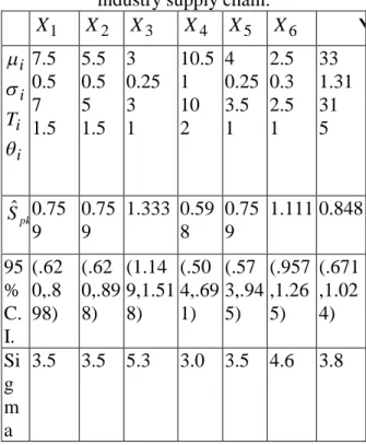
Figure 1. A linear supply chain model Example 1: Consider a supply chain in a TFT-LCD industry. Assume that there are six business processes: raw material procurement (X1), sub-manufacturing (X2), inbound logistics (X3), manufacturing (X4), final product assembly (X₅), and outbound logistics (X6). The known parameters are listed in Table 2. The sample size is 100. Let the target time and tolerance time for the supply chain delivery time be 31 days and 5 days, respectively. Using equations (1) and (2), we can show the delivery performance for this supply chain network in Table 2.

Table 2 Delivery performance in a TFT-LCD industry supply chain.

X

1

X

₂

X

₃

X

₄

X

₅

X

₆

Y

i i i i

T





 7.5

0.5 7 1.5

5.5 0.5 5 1.5

3 0.25 3 1

10.5 1 10 2

4 0.25 3.5 1

2.5 0.3 2.5 1

33 1.31 31 5

Sˆ0.75

pk

9

0.75 9

1.333 0.59 8

0.75 9

1.111 0.848

95

% C.

I.

(.62 0,.8 98)

(.62 0,.89 8)

(1.14 9,1.51 8)

(.50 4,.69 1)

(.57 3,.94 5)

(.957 ,1.26 5)

(.671 ,1.02 4) Si

g m a

3.5 3.5 5.3 3.0 3.5 4.6 3.8

A high value of

Sˆ

_pk implies a higher ranking of the process. In this TFT-LCD industry supply chain, inbound logistics

X

₃ is the highest ranked process whereas manufacturing

X

₄ is the lowest ranked process. The whole supply chain has only 3.8-sigma of the delivery performance. Based on the above analyses, improvement should focus on the manufacturing process. A TFT manufacturing process consists of array, cell, and module sub-processes (Jeong et al., 2002). Note that the TFT manufacturing process is very similar to semiconductor wafer fabrication, but is much simpler.

Deposition, photolithography and etching steps are common to both industries. The key differences are that the TFT is built on a glass substrate instead of a silicon wafer. In addition, the TFT requires a processing temperature ranging from approximately 300 to 500⁰F compared to the approximately 1,000 ⁰ F required for semiconductor fabrication. The module assembly process has very short lead times of approximately 8 hours compared to the first two stages with

7-8 days lead time. The features of the array process are the recycling of production and sharing of jointly finite facilities. Similarly, the considerations of the cell process are the availability of color filters. Thus, these two sub-processes can be classified into capacity-oriented production planning. In contrast, the module process considers the availability of key materials. Thus, it can be classified into material-oriented production planning. If a Six-Sigma project is employed to reduce the lead time of the manufacturing process, then the process mean and standard deviation of the manufacturing process are reduced to 10 and 0.75, respectively. Thus, the estimated value of

S

_pk becomes 0.889 with 95% confidence interval (0.766, 1.012).

Now, the estimated value of

S

_pk for the whole supply chain becomes 1.099 with a 95% confidence interval (0.894, 1.303). That is, the delivery performance of the whole supply chain can be improved from 3.9-sigma to 4.6-sigma.

4. Supplier Selection

Suppose that we have the processing cost per unit at each process i, denoted as

C , in the

_i supply chain. This cost is the part of the total processing cost that is associated with the delivery time. For example, in the case of a manufacturing process, it could be the opportunity cost of capital tied up with machinery. In addition, if it is a logistics process, then it may represent the cost of transportation itself. We suppose that the mean processing time for all potential service suppliers is almost the same but their variance may differ and hence per unit processing cost may also vary. Assume that the standard deviation



_iA,



_iB,of the processing time and the per unit processing cost

C

_iA,

C

_iB, are available for each of the service suppliers

A , B , 

for business process

i.

These pairs (



_iA,

C

_iA) ,

 ), ,

(



_iB

C

_iB can be used to obtain a polynomial function for the per unit

processing cost in terms of

 . Thus, the

_i unit processing cost for each process i is given as

2 2 1

0 i i i i

i

i

C C C

C     

(3)

where

C

_i0,

C

_i1,

C

_i2 are constants.

Given a supply chain and the mean and standard deviation of the end-to-end delivery time for a certain product, we can minimize the total processing cost and achieve the required delivery time performance through allocating the pool of variance among individual business processes. Then, these optimal variances for all business processes can be used to select suitable suppliers for the supply chain out of a given set of suppliers.

Thus, the problem formulation becomes:

Minimize

  

 

 

n i

i i i i i n

i

i

C C C

C TC

1

2 2 1

0 1





(4)

Subject to

S

_pk 

c

₀

i 0 

i



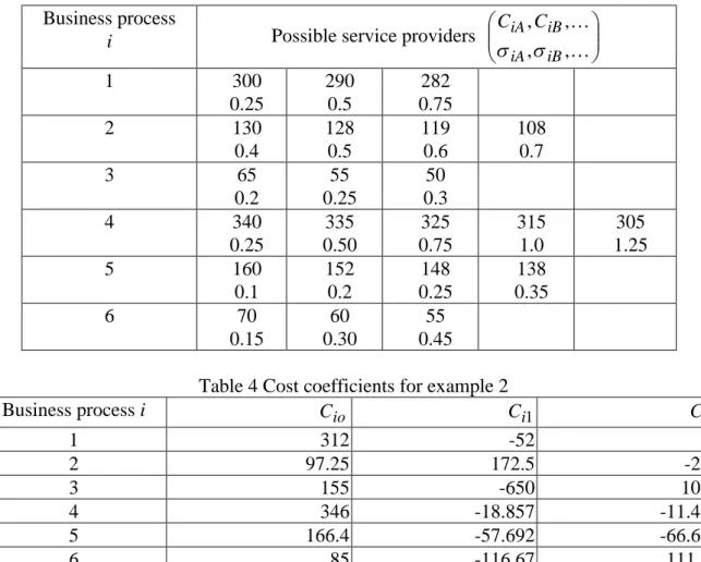
Example 2: Consider the previous example with the values of the per unit processing cost and the standard deviation of processing time for all potential service providers shown in Table 3. A second order polynomial curve fitting for the given pairs of cost and standard deviation for each process can be used to obtain the coefficients

C

_i0,

C

_i1,

C

_i2 . Thus, the cost coefficients are given in Table 4.

Here, the desire value

S

_pk of this supply chain is set at 1.55 which is equivalent to the 6-sigma level.

Table 3 Unit cost and standard deviation of delivery time for possible service providers

Business process

i

Possible service providers 



 







 , ,

, ,

iB iA

iB iA

C C





1 300

0.25

290 0.5

282 0.75

2 130

0.4

128 0.5

119 0.6

108 0.7

3 65

0.2

55 0.25

50 0.3

4 340

0.25

335 0.50

325 0.75

315 1.0

305 1.25

5 160

0.1

152 0.2

148 0.25

138 0.35

6 70

0.15

60 0.30

55 0.45

Table 4 Cost coefficients for example 2

Business process i

C

_io

C

_i1

C

_i2

1 312 -52 16

2 97.25 172.5 -225

3 155 -650 1000

4 346 -18.857 -11.429

5 166.4 -57.692 -66.697

6 85 -116.67 111.11

Using the data in example 1 and the coefficients in Table 4, the total processing cost is 995.77. The optimal suppliers in this supply chain can be solved by genetic algorithms as in the case of solving the total cost model in Evolver software (2001).

Genetic algorithms are highly effective in solving complex combinatorial problems in the fields of science and engineering. A complete description of their mathematical justification and good performance can be found in the work of Holland (1975). A genetic algorithm is a method of searching a set of solutions to identify the one that approaches a maximum value determined by an evaluation function. The biological genetics can inspire the mechanisms of the search algorithm, in which a population of organisms evolves to optimize its fit in an environmental niche (Glodberg, 1989). In this example, the crossover rate is set at 0.5, and the mutation rate is set at 0.1. The solution method is used by the recipe function. The population size is set at 50. The number of trials was set up to 10000 with 10 replications. The initial values for the standard deviation of each process are set at the values in example 1. The search procedure is repeated until the average objective function value for the current generation differs from that of the previous generation by less than 0.1%, or the best solution in the population has not changed for 10 subsequent generations. Once this termination condition is reached, the standard deviations for all processes are 0.209, 0.002, 0.270, 0.174, 0.428, and 0.336, respectively.

This is the lowest objective function value in terms of the total processing cost (= 982.09) selected as the best solution for the model. In this combination of the service providers, the value of

S

_pk is 1.56, which is equivalent to the 6-sigma level. The total processing cost can be improved by about 1.4%, and the sigma metric can be improved from 3.8-sigma to 6-sigma when the adjustments to the manufacturing process have been completed.

5. Conclusion

When a company attempts to improve the performance of its supply chain, it is crucial for it to understand the quality of the supply chain network. Six-Sigma is a systematic, data-driven approach to analyzing the root causes of business problems, and is a method for using such measures to analyze, improve, and control the overall quality of the supply chain network. When applying the capability index to delivery performance, the continuous improvement itself is a dynamic process of the supply chain network. Thus, improvement in the quality of all supply chain processes reduces costs and improves the level of customer service. When a Six-Sigma project is employed to reduce the lead time of the manufacturing process in a TFT-LCD supply chain, the process mean and standard deviation of the manufacturing process are reduced to 10 and 0.75, respectively. Thus, the delivery performance of the whole supply chain can be improved from 3.9-sigma to 4.6-sigma.

Six-Sigma is a new strategy to enhance the delivery performance of a supply chain network. It is believed that the integration of Six-Sigma into supply chain networks will become a standard practice for any e-business application that seeks an advantage in this highly competitive era of globalization.

Future research issue should focus on how to evaluate delivery performance in nonlinear supply chain networks.

References

1. Boyles R. A., The Taguchi capability index. Journal of Quality Technology, 1991, 23, 17-26.

2. Breyfogle, F. W., Implementing Six

Sigma: Smarter Solutions Using Statistical Methods, 1999 (Wiley, New

York).

3. Clarke, C. E., The greatest of a finite set of random variables. Operations

Research, 1961, 2, 145-161.

4. Erenguc, S. S., Simpson, N. C. and Vakharia, A. J., Integrated

production/distribution planning in

supply chains: an invited review.

European Journal of operations Research, 1999, 115, 219-236.

5. Evolver Software, Guide to Evolver, 2001 (Palisade Corporation, Newfield, NY).

6. Forker, L. B., Mendez, D. and Hershauer, J. C., Total quality management in the supply chain: what is its impact on performance, International Journal of

Production Research, 1997, 35,

1681-1701.

7. Goldberg, D. E., Genetic Algorithm in

Search, Optimization, and Machine Learning, 1989 (Addison-Wesley,

Reading, MA).

8. Harry, M. and Schroeder, R., Six Sigma:

The Breakthrough Strategy Revolutionizing the World’ s Top Corporations, 2000 (Doubleday, New

York,).

9. Holland, J., Adaptation in Natural and

Artificial Systems, 1975 (MIT Press,

Cambridge, MA).

10. Jeong B., Sim, S. B., Jeong, H. S. and Kim, S. W., An available-to-promise system for TFT LCD manufacturing in supply chain. Computer and Industrial Engineering, 2002, 43, 191-212.

11. Lee, J. C., Hung, H. N., Pearn, W. L., and Kueng, T. L., On the distribution of the estimated process yield index Spk. Quality

and Reliability Engineering International,

2002, 18, 111-116.

12. Sahner, R. A. and Trivedi, K. S.,

Performance and reliability analysis using directed acyclic graphs. IEEE

Transactions on Software Engineering,

1987, 13, 1005-1114.

13. Sculli, D., The completion time of PERT networks. Journal of Operational

Research Society, 1983, 34, 155-158.

14. Wang, F. K., Du, T. C. and Li, E. Y., Applying six-sigma to supplier

development. Total Quality Management

and Business Excellence, 2004, 15,

1217-1229.