行政院國家科學委員會專題研究計畫 成果報告
支援無線感測網路應用之致能技術及協定設計之研究(3/3) 研究成果報告(完整版)
計 畫 類 別 : 個別型
計 畫 編 號 : NSC 95-2221-E-011-085-
執 行 期 間 : 95 年 08 月 01 日至 96 年 07 月 31 日 執 行 單 位 : 國立臺灣科技大學電子工程系
計 畫 主 持 人 : 陳金蓮
計畫參與人員: 博士班研究生-兼任助理:許俊彥、陳建忠
碩士班研究生-兼任助理:詹益昇、吳志偉、侯玉祥、林依傑
報 告 附 件 : 出席國際會議研究心得報告及發表論文
處 理 方 式 : 本計畫可公開查詢
中 華 民 國 96 年 10 月 26 日
行政院國家科學委員會補助專題研究計畫成果報告
※※※※※※※※※※※※※※※※※※※※※※※※※※※※※※※※※※※※※
※ ※
※ ※
※ ※
※ ※
※ ※
※ ※
※※※※※※※※※※※※※※※※※※※※※※※※※※※※※※※※※※※※※
計畫類別:個別型計畫 □整合型計畫
計畫編號:NSC 95-2221-E-011-085
執行期限:93 年 8 月 1 日至 96 年 7 月 31 日
計畫主持人:陳金蓮 教授
計畫參與人員: 許俊彥 國立台灣科技大學 資訊工程研究所 陳建忠 國立台灣科技大學 電子工程研究所 詹益昇 國立台灣科技大學 電子工程研究所 吳志偉 國立台灣科技大學 電子工程研究所 侯玉祥 國立台灣科技大學 電子工程研究所 林依潔 國立台灣科技大學 電子工程研究所 本成果報告包括以下應繳交之附件:
□赴國外出差或研習心得報告一份
□赴大陸地區出差或研習心得報告一份
□出席國際學術會議心得報告及發表之論文各一份
□國際合作研究計畫國外研究報告書一份
執行單位:國立台灣科技大學 電子工程研究所
中 華 民 國 96 年 10 月 31 日
支援無線感測網路應用之致能技術及協定設計之研究 Research on Enabling Techniques and Communication
Protocols for Wireless Sensor Network Applications
行政院國家科學委員會專題研究計畫成果報告 支援無線感測網路應用之致能技術及協定設計之研究
Research on Enabling Techniques and Communication Protocols for Wireless Sensor Network Applications
計畫編號:NSC 95-2221-E-011-085 執行期限:93 年 8 月 1 日至 96 年 7 月 31 日
主持人:陳金蓮 教授 國立台灣科技大學 電子工程研究所
計畫參與人員: 許俊彥 國立台灣科技大學 資訊工程研究所
陳建忠 國立台灣科技大學 電子工程研究所
詹益昇 國立台灣科技大學 電子工程研究所
吳志偉 國立台灣科技大學 電子工程研究所
侯玉祥 國立台灣科技大學 電子工程研究所
林依潔 國立台灣科技大學 電子工程研究所
摘 要
無線感測節點具有通訊能力,可自 組成為一無線感測網路用以監測並蒐集 各種環境資訊,並可實際應用在醫療、
土木或軍事等等用途之上。由於無線感 測網路的感測節點數量多且密度大,其 路由協定常常受到擴充性(scalability)與 節點密度(node density)的限制,因此路由 協定必須另外特別設計。
本計畫在感測網路節點緊急訊息通 報的路由協定設計方面,以 Appointed BrOadcast (ABO)方法為基礎,設計了一 套協定能夠減低網路層找尋路徑時傳送 與接收封包花費的頻寬,並以模擬結果 說 明 其 性 能 , 藉 由 使 用 封 包 側 聽 (overhearing)的方式可明顯降低路徑發 現所需的代價。
此外,針對感測網路服務資訊散播 及資訊搜尋設計出資源散播及搜尋協 定,稱為 Simple Resource Advertisement and Discovery (SRAD),適合用於網路型 態大且稠密之無線感測網路,此協定可 使節點自我組織成一個完全分散式架構 的能力,模擬結果顯示在大量且密集的
無線感測網路中傳送訊息時,SRAD 協 定仍能達到不錯的效能。
為考量感測網路節點電源的管理,
以降低電能之消耗,本研究提出 throw and drowned (T&D) flooding protocol、叢 集式 cluster-based 演算法等協定,模擬結 果顯示此協定及演算法可達到省電及延 長網路的生命時間的目的。另外,針對 軟體無線電技術之應用,我們亦提出一 種讓無線感測網路中所有節點即時下 載、更新軟體的方法。
最後,我們另提出 cross-layer link adaptation (CLLA)及 CSMA protocol with collision avoidance, packing and accompanying (CSMA/CAPA)方法。模擬 結果顯示即使在資料錯誤率很高的情況 下,CSMA/CAPA 方法也能明顯提高網 路的 capacity,而 CLLA 方法在移動環境 中可以達到更高的流通量。
關 鍵 詞 : Appointed BrOadcast (ABO), SRAD, throw and drowned (T&D), cluster-based, SDR, CSMA/CAPA, CLLA
Abstract
Sensor nodes have to organize themselves into a connected network for acquiring and maintaining a reliable structure in the face of arbitrary topological changes. Such a structure must be achieved without the use of a central controller, that is, self-starting, and self-organizing algorithms must be developed to establish, control, and maintain a connected network in a transparent and distributed manner.
Because sensor nodes are usually equipped with small batteries with limited energy, energy saving is a critical issue.
Therefore, it is necessary to develop the architecture and protocols used in wireless sensor networks for the need of various wireless sensing tasks in the near future.
Besides, the feasibility of implementing software-defined radio (SDR), which allows one radio platform to service multiple standards, is another important research issue for wireless sensor networks.
In this project, several routing protocols and methods are proposed. We have studied the ABO method for emergency event message routing, the Simple Resource advertisement and discovery (SRAD) in WSNs, and the energy-saving cluster-based algorithm for networked sensors. Simulation results show using the ABO method can significantly reduce the cost on route discoveries, the SRAD protocol can achieve the same level of performance as in the broadcast-based protocols while generating fewer transmitted messages in large and dense WSNs. And the cluster-based algorithm can save energy consumption to prolong network lifetime, while achieving a low sensing coverage loss ratio.
We also studied an energy-efficient multi-hop implicit routing method, called
throw and drowned (T&D) flooding protocol,
which has threefold mechanisms for power-saving. The Carrier Sense Multiple Access protocol with Collision Avoidance, Packing and Accompanying (CSMA/CAPA) protocol , Packing packets can significantly reduce the access delay and loss rate. A cross-layer link adaptation (CLLA) schemethat uses the number of successful transmissions, the number of transmission failures, and the channel information from the physical layer to determine proper transmission parameters for subsequent medium accesses.
Keywords: Appointed BrOadcast (ABO),
SRAD, throw and drowned (T&D), cluster-based, SDR, CSMA/CAPA, CLLA一、緣由與目的
In wireless sensor networks (WSNs), sensor nodes that intend to access a data sink have to discover routes to the sink node first, which may result in considerable bandwidth cost. We studied the cross-layer design of the Appointed BrOadcast (ABO) method in order to reduce the cost of route discovery in WSNs. Besides, to consider the widespread use of legacy IEEE 802.11 nodes, the coexistence problem of how ABO-enhanced and legacy IEEE 802.11 nodes can coexist is also studied.
Because the geographical sensor network environments may be large and dense. In such network environments, a large number of resource discovery queries may be generated when specific resources or services are needed. In order to effectively utilize the limited bandwidth of the networks, and reduce power used by mobile devices, the design for resource discovery protocols should take both the operational cost and the network performance into account.
Moreover, the results of resource discoveries may further be used in later route discovery processes of certain routing protocols. We propose a simple resource advertisement and discovery (SRAD) protocol which self-organizes a proximity network and works in a fully distributed architecture without centralized control or management to prevent performance bottleneck. In addition, a resource description and management scheme is also devised to share loads among nodes.
We studied an energy-efficient
multi-hop implicit routing method, called
throw and drowned (T&D) flooding protocol,
which has threefold mechanisms for power-saving. First, T&D is capable of turning sensor node into sleeping mode to save power. Second, T&D is designed as a flooding-based and implicit routing protocol.Last,T&D uses“link-layer-relaying”instead of“network-layer-forwarding.” Mostofthe sensing tasks require knowledge of location information and part of WSNs routing protocol requires the assistance of location information. The T&D does not use the sensor node’slocation information.However, it can be applied to the applications whether they have the location information or not.
The software-defined radio (SDR) technology provides software control of a variety of modulation techniques, wide and narrow band operations, communication security functions, and waveform requirements of current and evolving standards over a broad frequency range. An SDR reconfigurable device is able to combine a software programmable processor and reconfigurable hardware components that can be reused for different applications.
Software downloading is the delivery of reconfiguration data or new executable codes to an SDR device to modify its behavior or performance. In a multi-hop SDR reconfigurable network, nodes may be reconfigured while they are working. An intuitive method for software delivery is to broadcast software to each node via flooding.
However, in this way, a serious problem will occur during the flooding process. If a node receives new software and turns itself into new mode that works in another communication protocol right after it forwards the software, the network will then be partitioned, and the flooding procedure is no longer effective. To avoid this problem, we propose a download scheme for real-time software download, application software upgrades, or radio protocol changing of wireless nodes.
In the IEEE 802.11 standard, an access point (AP) acts as the gateway or a sink node.
The carrier sense multiple access with
collision avoidance (CSMA/CA) protocol suffers from contentions that the system performance degrades rapidly with increasing number of active sessions. Note that in DCF, all nodes have the same transmission priority. Since the packet arrival rate of downstream traffics at the AP is generally higher than that of upstream traffics at a node. As the number of active sessions increases, both the loss rate and delay of downstream traffics rise rapidly, which limits the number of active sessions the network can support. We propose the Carrier Sense Multiple Access protocol with Collision Avoidance, Packing and Accompanying (CSMA/CAPA) protocol.
The packing scheme is employed to upgrade network capacity, and the accompanying scheme can mitigate packet loss rate and delay difference between upstream and downstream traffics. Packing packets can significantly reduce the access delay and loss rate. The accompanying scheme allows nodes to transmit a DATA frame after having received a DATA frame, so that upstream and downstream traffics can have balanced transmission opportunities.
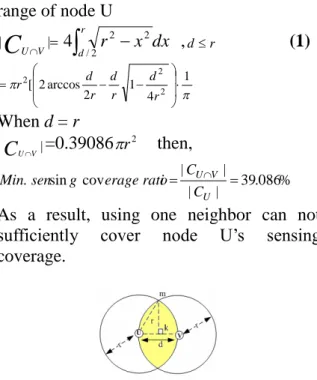
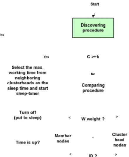
We study the off-duty role to turn off some redundant sensor nodes in order to let a large sensor network maintain long network lifetime while having low sensing coverage loss. We propose a cluster-based scheme to find sensor nodes with larger number of neighboring sensor nodes and remaining lifetime in their sensing coverage, which may possibly be elected as a cluster head node. A cluster head node has to perform sensing tasks, and other nodes are served as redundant nodes if they can be covered by several cluster head nodes.
In order to improve the throughput of a wireless network, dynamic link adaptation schemes can be applied so that the signal and protocol parameters can be adjusted as the radio link conditions change, according to the quality of a wireless channel. Receiver's signal-to-noise ratio (SNR) and received signal level (RSL) are two critical performance parameters that vary with time due to path loss, shadowing effect,
multi-path fading and interference. Hence, according to the SNR and RSL of the latest received frame, a link adaptation scheme can quickly respond to the channel variation and suitably adjust parameters for transmissions.
We hence propose a cross-layer link adaptation (CLLA) scheme that uses the number of successful transmissions, the number of transmission failures, and the channel information from the physical layer to determine proper transmission parameters for subsequent medium accesses.
In these three years, we have studied the above seven topics. Simulation studies are provided in the following sections.
二、結果與討論 I. ABO Method
1. Simulation model
In the simulation, we tested two typical routing protocols based on two different concepts: DSR and AODV, and three different MAC protocols: legacy IEEE 802.11, ABO and promiscuous mode. In DSR, the route is specified by the source node in the packet header while in AODV, the destination node address is the only guidance to which the packet should be forwarded. Both the routing protocols are enhanced to employ the ABO method and to handle overheard packet properly. A variation of the ABO method by releasing the AFP scheme will have similar performance as the promiscuous mode because all control messages will be overheard by neighboring nodes. The only difference between using the AFP-released ABO method and using promiscuous mode is that nodes using promiscuous mode overhear data packet while nodes using the AFP-released ABO method do not. We employ the
expending ring search
mechanism, which is specified in both AODV and DSR, to reduce the number of RREQ messages in the network.Unicast control messages, including RREP and RERR messages, are selected to
transmit using the ABO method. The defer time D
RREP
is based on the following function:D RREP
= H
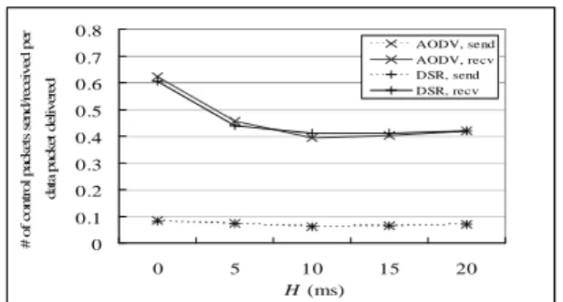
(h-1+r)where H is a small constant delay, h denotes the number of hops along the route being replied, and r is a random number uniformly distributed between 0 and 1. It is suggested that H is at least twice the maximum wireless link propagation delay. We evaluated the impact of different H values as shown in Figure 1 and find that when H is 10ms, the control cost is the lowest.
The channel bit rate is 2 Mb/s and the radio range is 250 meters. A sink node is placed at the center of the simulation area where 50 nodes are placed randomly. Three scenarios are studied: 300
1500 m2
, 600
1500 m2
and 1000
1000 m2
.0 0.1 0.2 0.3 0.4 0.5 0.6 0.7 0.8
0 5 10 15 20
H (ms)
#ofcontrolpacketssend/receivedper datapacketdelivered
AODV, send AODV, recv DSR, send DSR, recv
Figure 1. Different deferring delay (pause time=300s, CBR sources=25, MAC=ABO)
The data packet size is 512 bytes and the inter-arrival time of packets is 0.4 second.
The simulation time is 900 seconds. The random waypoint model is used for the mobility model. Each node is independent and no group movement is presented. Nodes are stationary (i.e., no mobility is presented) for a period of time t
pause
at the beginning of simulation. tpause
is exponentially distributed with a mean pause time. Larger mean pause time means more stationary nodes and lower topology-changing rate. When tpause
times out, the node will move to a randomly selected new location with a moving speed uniformly distributed with a range of (0, 20) m/s. When the node reaches the new location, it picks a new tpause
value and remains stationary before tpause
times out. The pause time ranges from 0 to 900 seconds. Note that a zero pause time implies that nodes arealways moving and the network topology is highly dynamic, while pause time of 900 seconds implies that all nodes are stationary during simulation. For fair comparisons, the mobility and traffic patterns are the same among the compared protocols. The presented simulation results come from a mean of 50 runs.
2. Performance comparisons
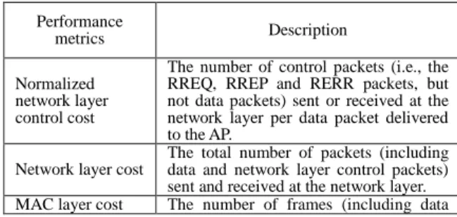
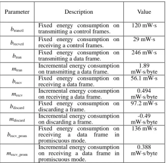
Table 1 summarizes performance metrics that are used for comparisons. Since the sink node is assumed to have no energy concerns, the cost spent by the sink node to send or receive packets and frames is not included in the simulation results. In this way, we emphasize on the costs incurred in mobile nodes. Power consumption in memory access is not considered since it is insignificant compared with that of CPU operations and wireless transmissions. CPU time required for four packet lengths are 100, 192, 500 and 1000 bytes, respectively. We supplement the CPU time required for other packet lengths by linear regression as depicted in Figure 2. The model developed by Feeney, where the corresponding parameters are given in Table 2, is used to measure the energy consumption at the MAC layer.
At the transmitter,
b tranctl
+ brecvctl
+ mtran
×size + btran
+ brecvctl
. At the destination node of the data frame,b recvctl
+ btranctl
+ mrecv
×size + brecv
+ btranctl
. At non-destination node that discards the frame,
D n T
n
D n T
n
b b
size m
b b
discardctl discard
discard
discardctl discardctl
) (
At non-destination node that operating in promiscuous mode,
D n T
n
D n T
n
b b
size m
b b
discardctl recv_prom
recv_prom
discardctl discardctl
) (
where T and D denote respectively the set of neighboring node of the transmitting and destination nodes.
0 100 200 300 400 500 600 700
0 100 192 500 1000
packet length (Bytes)
pr oc es si ng ti m e (μ s)
receiving sending
Figure 2. Processing time required with respect to packet length
Figure 1 shows the normalized network layer control cost using different H values.
H=0 implies that nodes do not defer before
replying RREP message back to the source node. An underestimated H value cannot prevent the network from the reply storm problem. On the contrary, an overestimatedH value may result in the source node route
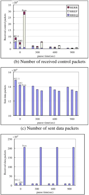
discovery times out, and then route discovery is initiated again, which introduces more number of control messages. In the following, only the result of AODV is presented.Figure 3 compares the number of control and data packets sent and received using the three MAC protocols. Note that even when all nodes are stationary (pause time=900s), a small amount of RERR messages are issued.
This is because, sometimes, the MAC layer transmits a frame but receives no ACK because of collisions. The MAC layer will retry until an ACK is received or the retry limit is reached. If the latter occurs, the MAC layer will signal the network layer that the wireless link is not available. The network layer then recognizes this as a route failure and initiates an RERR message to the corresponding source nodes.
Table 1 Performance metrics used in simulations Performance
metrics Description
Normalized network layer control cost
The number of control packets (i.e., the RREQ, RREP and RERR packets, but not data packets) sent or received at the network layer per data packet delivered to the AP.
Network layer cost
The total number of packets (including data and network layer control packets) sent and received at the network layer.
MAC layer cost The number of frames (including data
and MAC layer control frames) sent and received at the MAC layer.
Normalized CPU time
Required CPU time at the network layer per data packet delivered to the AP.
Normalized energy consumption
Energy consumed at the MAC layer per data packet delivered to the AP.
Packet delivery ratio
The number of data packets received by the sink node to the number of packets generated by all traffic sources.
Average end-to-end data packet delay
The average end-to-end delay of data packets.
Table 2 Energy consumption parameters
Parameter Description Value
b
tranctlFixed energy consumption on transmitting a control frames.
120 mW·s
b
recvctlFixed energy consumption on
receiving a control frames.
29 mW·s b
tranFixed energy consumption on
transmitting a data frame.
246 mW·s m
tranIncremental energy consumption
on transmitting a data frame.
1.89 mW·s/byte b
recvFixed energy consumption on
receiving a data frame.
56.1 mW·s m
recvIncremental energy consumption
on receiving a data frame.
0.494 mW·s/byte
b
discardFixed energy consumption on
discarding a frame.
97.2 mW·s
m
discardIncremental energy consumption
on discarding a frame.
-0.49 mW·s/byte b
recv_promFixed energy consumption on receiving a data frame in promiscuous mode.
136 mW·s
m
recv_promIncremental energy consumption on receiving a data frame in promiscuous mode.
0.388 mW·s/byte
In Figure 3(a), compared to legacy IEEE 802.11 MAC, using the ABO method can significantly reduce the number of control packets. Using promiscuous mode can obtain even more improvements. As shown in Figure 3(b), using promiscuous mode results in a large number of control packets arrived at the network layer since the MAC layer does not filter out frames. On the contrary, the network layer receives the least number of control packets when the ABO method is employed, because when the ABO method is used, only those packets that are carried by ABO frames (unicast RREP and RERR messages in this case) can be overheard by the network layer. Note that the AFP scheme limits the frequency on using the ABO frame, so when the ABO method is used, the number of control packets arrived at the network layer is less than that when promiscuous mode is used. On the other hand, compared with legacy IEEE 802.11 MAC, the ABO method issues 50% less control packets as shown in Figure 3(a). The
reduction of control packets can compensate the increased number of received control packets caused by the use of the ABO frames.
The number of control packets arrived at the network layer of the ABO method is less than that of the legacy IEEE 802.11 MAC.
Although using promiscuous mode results in the least cost on sending data packets as shown in Figures 3(c), a large number of data packets are received at the network layer -- about 20 times as many as that of using the legacy IEEE 802.11 MAC and the ABO method as depicted in Figure 3(d).
This is inevitable because using promiscuous mode, the MAC layer receives data frames and passes all of them to the upper layer without filtering. The result indicates that nodes using promiscuous mode have to spend much more computation power to deal with the overheard packets, as shown in Figure 4.
Figure 5 depicts the simulation results on the number of frames transmitted/received at the MAC layer. The number of frames transmitted is directly related to the number of packets sent at the network layer, and the number of frames received is directly related to the number of frames transmitted.
Because promiscuous mode has the least number of control packets issued, it introduces the least number of frames transmitted/received at the MAC layer.
However, less number of
transmitted/received frames does not always imply lower energy consumption.
0 0.5 1 1.5 2 2.5 3
0 300 600 900
pause time(sec)
Sentcontrolpackets|
RERR RREP RREQ
(a) Number of sent control packets
0 5 10 15 20 25 30 35
0 300 600 900
pause time(sec)
Receivedcontrolpackets|
RERR RREP RREQ
(b) Number of received control packets
10 12 14 16
0 300 600 900
pause time(sec)
Sentdatapackets|
Prom ABO 802.11
(c) Number of sent data packets
0 50 100 150 200 250
0 300 600 900
pause time(sec)
R ec ei v ed d at a p ac k et s |
Prom
ABO 802.11
(d) Number of received data packets Figure 3. Network layer costs (CBR sources=25)
0 2000 4000 6000 8000 10000 12000 14000
0 300 600 900
Pause time (sec)
CPUtime(μs)
Recv data Recv ctrl Send data Send ctrl Prom
802.11ABO
Figure 4. Normalized CPU time
0 10 20 30 40 50 60 70 80
0 300 600 900
pause time(sec)
S en t fr am es
Control ABO Unicast Broadcast Prom
802.11
ABO
(a) Number of transmitted frames
0 200 400 600 800 1000 1200 1400
0 300 600 900
pause time(sec)
R ec ei v ed fr am es
Control ABO Unicast Broadcast Prom
ABO 802.11
(b) Number of received frames
Figure 5. MAC layer costs (CBR sources=25)
II. The SRAD Protocol
If a resource discovery protocol heavily relies on network-wide broadcast, nodes will experience considerable power consumption.
Besides, resource discovery mechanism must be designed properly so that users can discover the resource efficiently while the cost is minimized. We assume that nodes have the capability of location awareness.
1. Resource description and management In the application layer, the location information of a restaurant, for example, can be described using a resource descriptor in this form: < information-orient. location.
restaurant >. Then, the resource descriptor is
encoded as a 128-bit resource key using the MD5 algorithm. In this way, a resource descriptor can be encoded as a unique number called resource key.The SRAD protocol is devised to let server nodes advertise their resource
information along one of the twenty line trajectories uniformly distributed on a plane.
Hence, the resource key will then be used to determine a direction (or angle) for information dissemination using a hashing function. To do so, the modulo-k scheme is chosen as the hashing function. We let k be 20 to divide 180 degrees into 20 parts. Then, using the tangent function, we can easily get a slope of a line trajectory. Here we call it the main slope (S
m
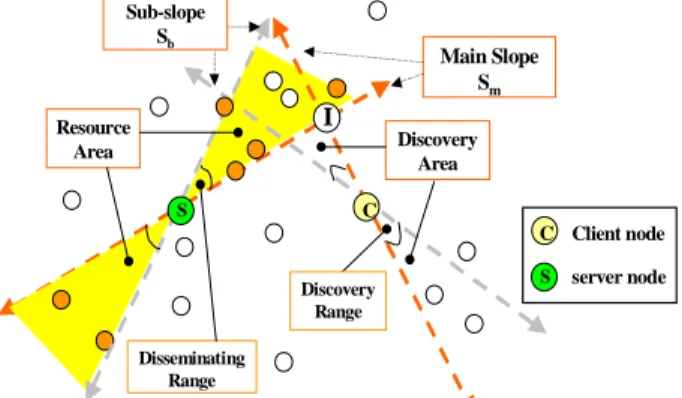
).2. Resource description and management As shown in Figure 6 the resource advertisement is performed on the basis of the line trajectory with main slope and a tolerance that forms a resource area. Nodes that lie within the resource area must cache the resource information. Resource discovery is performed on the basis of another perpendicular line trajectory that forms a discovery area. Note that the
disseminating range is a tolerance of an
angle to allow the resource information to be disseminated. The discovery range is a tolerance of an angle to allow the resource information to be discovered. If a node in both resource area and discovery area has the resource information, or a node coming from the resource area just moves to the discovery area holds the resource information, it must send a reply to the client node.2.1 Line-based (LB ) SRAD A. Resource advertisement
The server node advertises its resource information using an advertisement (ADV) packet every T
interval
seconds. Tinterval
depends on the speed of the mobile node, in a highly dynamic situation, it is desirable to have a small Tinterval
. The ADV packet contains the following fields:< Packet type, Source ID, Server’s Coordinate, Sequence Number, Resource Key, Hop Count, Lifetime, Main Slope >
The Hop Count field is used as hop count limitation that confines the distance an ADV can travel. The Source ID and Sequence
Number fields are used to distinguish duplicate advertisements. The Lifetime field in ADV packet defines the lifetime of the resource information to be cached. High mobility server nodes in a WSN will set a small lifetime for this resource entry. This cached resource entry would be deleted once its lifetime expires. Each entry in the cache contains the following fields:
< Server ID, Resource Key, Server’s Coordinate, Previous ID, Sequence Number, Lifetime >
When a node receives an ADV packet with new sequence number, it calculates whether itself lies in the resource area or not.
If true, the resource information is recorded in the cache for a specified lifetime. Then, the node decrements the value of the Hop Count field in the ADV packet by one, and broadcasts it again if the value of Hop Count is larger than zero; otherwise, the ADV packet is discarded. Because an ADV packet keeps the server’s coordinate and the main slope of a line trajectory, a node can determine whether itself is located in the resource area by some calculations.
This advertisement process will be carried out until the value of Hop Count field in the ADV packet reaches zero. In this way, the ADV packet is broadcasted within a confined resource area roughly along a line trajectory to avoid flooding the network.
S
Main Slope S
mSub-slope
S
bResource Area
I
Disseminating Range
C
C S
Client node server node Discovery
Area
Discovery Range
Figure 6 Resource area and discovery area.
B. Resource Discovery
When a client wants to find a resource or service, it first checks if it has cached the resource information that has not expired. If false, it calculates the resource key using the
encoding process. Thus, the client can obtain the same resource key as what server obtains.
Using that resource key, the client node can calculate the main slope of a line trajectory to disseminate a resource request (RREQ) packet for resource discovery.
The client firstly generates a RREQ packet and initiates the resource discovery process.
Note that for resource discovery, the RREQ packet is disseminated along a line trajectory perpendicular to the line trajectory used in the resource advertisement process. The nodes that lie in both the resource area and discovery area can send a resource reply (RREP) packet to the client node using unicast to complete the resource discovery process. Moreover, if a node coming from the resource area just moves to the discovery area, it will also send a RREP packet to the client node. The RREP packet consists of the following fields:
< Packet type, Sequence Number, Server’s ID, Server’s Coordinate, Resource Key, Hop Count, Coordinate of the Reply Node, Main Slope, Lifetime >
When a node receives a RREQ packet, it first checks whether the RREQ packet is a duplicated one. If true, the RREQ packet is discarded. Otherwise, if it has cached the resource information, it then sends back a RREP packet directly to complete the resource discovery process, or else it then determines whether or not itself lies in the discovery area using geometry calculations.
If the node lies in the discovery area and does not have the desired resource information, then, the node decrements the value of the Hop Count field in the RREQ packet by one, and broadcasts it again if the value of Hop Count is larger than zero;
otherwise, the RREQ packet is discarded. A resource discovery process fails if the client node does not receive the RREP packet within T
RTT
, the maximum tolerable round trip time. TRTT
is set according to the average number of hops the RREQ packet is expected to travel. If resource discovery processes fail frequently, TRTT
and the value of the Hop Count field in the RREQ packets can be set larger.2.2 Enhanced line-based (ELB) SRAD It is possible that a server is located at the geographical border of the network and no neighboring node lies on the discovery trajectory or resource area. Besides, because the geometric coverage area near the server is small, some nodes may be close to the server but could not recognize the resources of the server. Hence, the enhanced line-based (ELB) SRAD protocol is proposed. The ELB protocol uses two main slopes that form two line trajectories perpendicular to each other to disseminate the ADV and RREQ packets.
In the ELB protocol, the resource discovery process is the same as that of the LB protocol based on one selected main slope. But if the first resource discovery process fails, the client node will try to send another RREQ packet using the other main slope.
2.3 Cross-line-based (CLB) SRAD
To increase hit rate and consider that nodes may not be uniformly distributed in the network, the cross-line-based (CLB) SRAD protocol is proposed. In the CLB protocol, the resource advertisement process is the same as that of the ELB protocol based on two main slopes. But the former discovers resource based on two main slopes at the same time. The performance penalty of the CLB protocol is that the transmitted message overhead is more than that of the ELB protocol since it discovers resource along two line trajectories.
3. Simulation study
For comparisons, an on-demand (OD) resource discovery protocol modified from the AODV routing protocol to support resource discovery is implemented in simulations. The performance metrics to be observed include:
Number of transmitted messages: the total
number of broadcast messages in the network. Average hit rate: the ratio of the total
number of successful resource discoveries to the total number of queries. Average hop-count:
the number of hop-counts between the client nodes and the reply node that is located at the discovery area.4. Simulation metrics
The simulation parameters are summarized in Table 3. The disseminating range and discovery range are tolerances of angle in degrees to allow the resource information to be disseminated and discovered as shown in Figure 6.
Table 3 Simulation parameters Environment
Parameters
Highly dense Large and dense Simulation region 500m x 500m 1000m x 1000m Total number of nodes 100 to 500 1000 Speed of node (km/hr) 7.2 to 57.6 7.2 to 57.6
Radio coverage (meter) 100 100
Number of server nodes 1 1
Disseminating range 18
018
0Discovery range 18
0and 36
018
0Number of client nodes 30 30
T
interval(second) 50 50
T
RTT(msec) 100 100
Hop Count 3 6
5. A comprehensive comparison
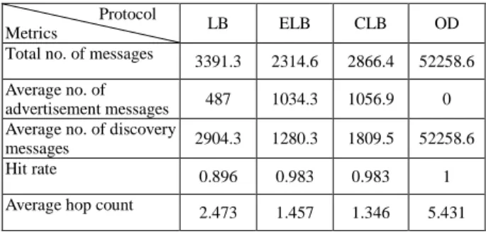
Table 4 shows the comparison of various metrics in terms of average total number of transmitted messages, average number of advertisement and discovery messages, average hit rate, and average hop count for OD and the three SRAD protocols for large and dense network environment. The result shows that about 52,258 transmitted messages are generated using the OD protocol. Nevertheless, using the LB protocol guarantees a hit rate of 89.6% and its overhead is only 6.5% of that of the OD protocol. Because in ELB and CLB protocols, more nodes may have cached the advertised resource information and can send a reply directly to the source of query in the discovery process, these two protocols generate fewer messages in the network than the LB protocol does. Hence, using the ELB and CLB protocols guarantees a hit rate of 98.3% and their overhead are respectively
4.4% and 5.5% of that of the OD protocol.
Table 4 Comparison of various performance metrics with 1000 nodes
Protocol
Metrics LB ELB CLB OD
Total no. of messages 3391.3 2314.6 2866.4 52258.6 Average no. of
advertisement messages 487 1034.3 1056.9 0 Average no. of discovery
messages 2904.3 1280.3 1809.5 52258.6
Hit rate 0.896 0.983 0.983 1
Average hop count 2.473 1.457 1.346 5.431
III. The T&D Flooding Protocol
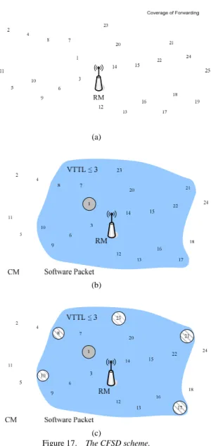
T&D divides time into slots and intends to propagate one packet in a slot. Any node receives a packet and throws it after a random backoff time by broadcasting. Nodes receiving more than one packet will be
drowned by the packet and stop throwing it.
T&D needs not to maintain the neighbors table during the packet relaying stage, and it may have more than one route propagating the packet to the sink
.
T&D consists of two parts: medium allocation and medium access control (MAC). The related network management and security functions are centralized and controlled by the sinks, which is out of scope of this study. The MAC function of T&D is based on the carrier sense multiple access with collision avoidance (CSMA/CA). And it is modified from the IEEE 802.11 distributed coordination function (DCF). We call the MAC as T&D-MAC.
3.1 Medium Allocation
Information gathering in WSNs is typical in two manners and referred to proactive and reactive approach, respectively.
In proactive approach, sensor nodes transmit sensed data periodically to the sinks. In the reactive approach, remote users originate a query to the WSNs for response when they are interested in some information. The query generally is attribute-based addressing and those nodes that satisfy the query will respond to it.
Figure 7 depicts the medium allocation method of T&D. The time is equally divided by packet propagation period (PPP). A number of PPPs comprise a super frame.
T&D is designed to carry one packet per PPP. However, due to the contention-based MAC protocol, T&D has the probability to transmit either none or more than one packet from individual sensor node to sink in a PPP.
The first PPP in a super frame is a control
PPP reserved for
monitoring/management/query packets. Sink or remote user uses the control PPP to send monitoring/management/query packets to sensor nodes. The other PPPs are data PPPs which sensor nodes use to transmit their periodically reports or response the query to the sink. The number of PPPs comprising a super frame is a managerial parameter depending on the load of network signaling and queries. The length of a PPP is also a system parameter whose duration is a value between [PPP_min, PPP_max]. PPP_min must be long enough to propagate a packet from any sensor node to sinks, which is dependent on the scale of WSN. When data load gets higher, the PPP can be shortened down to the PPP_min to adopt these loads.
On the other hands, when data load gets lower, the PPP can be prolonged for power saving.
3.2 T&D-MAC
Theterminology “frame”is used to be the data unit in MAC layer. Here we assume that a data packet in the WSN can be completely encapsulated in a frame.
Therefore, theterms“frame”and “packet”is interchangeable in this study.
A sensor node acts in three states:
contention state, relaying state, and sleeping state, during a PPP. Figure 8 illustrates the state transition diagram of a sensor node.
And the tasks performed by a sensor node during a PPP are shown in Figure 9. For each state, the activation of each subsystem of a sensor node is tabulated in Table 4. The start state of all sensor nodes is the sleeping state. When a data PPP starts, a sensor node turns to contention state if it has a packet
want to send to sink. Otherwise, it turns to relaying state directly. Sensor nodes which are in contention state select a backoff time (BT) in units of slot times and decreases the backoff time by one until to zero. When the backoff time is decreased to zero, a sensor node transmits the packet and turns to the sleeping state until next PPP starts. If sensor nodes fail in contending the channel, i.e.,the nodes receive a packet during the backoff procedure, they freeze the backoff time and turn their state to relaying state.
Sensor nodes which are in relaying state monitor the channel until the PPP_min expired. If they receive a frame by PPP_min, they perform the relaying procedure. The relaying procedure is identical to the backoff procedure using in the contention stage;
however, the contention window (CW) size may different and the backoff counter will be reset every relaying stage. Moreover, the sensor node should wait a inter frame space (IFS) before random backoff. After relaying a packet, sensor nodes turn into the sleeping state. If a sensor node is in relaying stage and receives more than one packet, regardless of duplicating packets or different packets, before successfully relaying any packet. We say that the node is drowned by packets, and then the node stops relaying any packet and turns to the sleeping state.
Because the T&D is designed to use
“link-layer-relaying” instead of
“network-layer- forwarding,” the sensor node will not cache any packet and, except the MAC address resolution and check sum, the sensor node will not perform any header check. In addition, sensor nodes use only one cache for cooperating packet routing.
Because that sensor nodes use contention-based channel access scheme, collision may occur in contention stage and relaying stage. If a sensor node detects collision occurred, it simply turns to sleeping state until next PPP starts. However, collision will not significantly affect the packet propagation. For example, in Figure 10, if node A and node B transmit packets simultaneously, node C will detect collision and turns its state to sleeping state. However,
node D and node E will relay these packets to their neighbors, respectively. In the sleeping state, the sensor nodes will turn off their radio circuits (including listening function) and then isolate themselves from the network to save battery power.
3.3 Simulation Results and discussion
A. Simulation Environment
A sensor field with 500 500 square meters and acting as proactive mode is considered. Sensor nodes reporting the collected data follows the exponential distribution with mean interarrival time 30 minutes. The traffic load is a function of the density of the sensor networks, denoted as , which can be calculated as(R) = (N R2) /
A, where N is the number of sensor nodes, R
is the radio transmission range of a sensor node, and A is the area of sensor field.Node’s move isaccording to the “random waypoint”model.The movingspeed of each node is assumed to be uniformly distributed between [0.3, 2] m/s, and the pause time is assumed to be 100 s. The number of sinks is assumed to be 1, 2 and 4 sinks in the sensor field. They are at fixed positions and are shown in Figure 11.
The pure flooding and Gossiping scheme are also simulated. The MAC of these schemes is identical to the DCF of IEEE 802.11. In the pure flooding scheme, the duplication check is performed when receiving frames, so that any packet will be rebroadcast only once in each node.
However, the positive ACK and collision-aware retransmission scheme are skipped. In the Gossiping scheme, the sensor node randomly chooses a neighbor to transmit the packet. The cost for maintaining the neighbors ID table at a sensor node is omitted. The duration of processor to be waked up for duplication check or next hop selection is assumed to be uniformly distributed between [50, 100] s. We perform this simulation by create a dedicated simulator using C language.
In order to estimate physical power
dissipation, the WINS node characteristic is adopted in this simulation and is tabulated in Table 5. The cost using in the sensing subsystem is omitted. Other parameters used in the simulation are tabulated in Table 6.
B. Simulation results and discussion
Three metrics are interested and simulated: packet reachability, packet delay, and WSNs’ lifetime. To simulate thefirst two metrics, we assume that the power of sensor node is infinitive and the simulation time is 50,000 s. The packet reachability is defined as the proportion of received packets to the transmitted packets and illustrated in Figure 12. The numbers of sensor nodes from 80 to 800, i.e., the densities of sensor nodes from 10.05 to 100.5, are simulated. In other words, a sensor node has 10.05 to 100.5 neighbors in average. Therefore, the packet loss due to network partition is rare.
Packet loss in pure flooding scheme is mainly caused by collision. When the number of sensor node increases, the collision increases. Thus the reachability degrades. The very low reachability of Gossiping shown in Figure 12 is because that a large part of packets are seeking the road to the sink when simulation time expiration. The T&D has good reachability when the sink number is increased. In four sinks condition, the reachability of T&D exceeds pure flooding due to fewer collisions than the flooding scheme.
Figure 13 shows the packet delay of each scheme. The increasing delay in pure flooding when number of sensor nodes increase is because longer contention delays in a crowded channel. The average delay of the T&D is almost constant and dependent on the length of a PPP.
To simulate the WSNs’ lifetime, the energy in each sensor node is assumed to be 5,000 joules. And the lifetime is simply defined as the time when half sensor nodes in the WSN exhausting its energy. As shown in Figure 14, the T&D has longest lifetime than the other two schemes. The most reason is because T&D capable of turning sensor node to sleeping state. On the other hand, the
pure flooding and Gossiping scheme has the almost same lifetime is because they listen the channel all the lifetime. The length of a PPP is a managerial parameter, which is selected according to the tradeoff among the traffic load, packet delay, and WSN’s lifetime.