行政院國家科學委員會專題研究計畫 成果報告
子計畫一:特定疾病版生活品質問卷的發展與結構分析
(3/3)
計畫類別: 整合型計畫 計畫編號: NSC91-2320-B-002-083-M56 執行期間: 91 年 08 月 01 日至 92 年 07 月 31 日 執行單位: 國立臺灣大學心理學系暨研究所 計畫主持人: 姚開屏 報告類型: 完整報告 處理方式: 本計畫可公開查詢中 華 民 國 92 年 10 月 22 日
2 此篇國科會研究計畫結案報告包括了兩篇研究, 研究一:不同疾病患者生活品質因素結構之比較 研究二:我們能嗎?誰可以?該如何?對生活品質測量之向度做加權
第一篇研究摘要
本篇的目的是想探討不同疾病患者對生活品質看法之差異。我們使用了過去 從全台灣十七家醫院隨機收集到的一千多位健康人與病人的資料,取其中有較多 病人的幾種疾病,再加上後來收集到的一百八十一位冠狀動脈繞道手術的病人的 資料,來分析健康人與病人之間的差異,以及不同疾病病人之間的差異。分析的 方法採探索性因素分析(exploratory factor analysis)及驗證性因素分析 (confirmatory factor analysis)於四因子模式,以比較不同組別間的差別。 在比較探索性因素分析二獨立組間因素結構相似度方面,採計算因素適合係數 (factor congruence coefficient)的方式。在用驗證性因素分析用於四因子 模式因素結構可比較性方面,採多樣本分析(multi-sample analysis)的方法, 以確認因素結構間之可比較性。研究結果顯示,不同組別的確對生活品質的看法 不相似。詳細內容請見研究論文。 關鍵詞:生活品質、因素結構、探索性因素分析、驗證性因素分析第二篇研究摘要
本篇的目的是探討對生活品質量表各向度加權的方式。我們從根本的角度 來談這個問題,而問了三個問題。第一個問題是「我們能對生活品質量表各向度 做加權嗎?」,這個問題的答案依著我們採何種方式來定義生活品質而定。在某 種定義下,我們的確可對生活品質量表各向度做加權(詳見論文內文)。第二個 問題是如果第一個問題的答案是肯定的,則繼續問「誰能做加權?」,是醫療健 康人員?病人?醫療政策制訂者?還是社會大眾?本研究從不同角度來談,在不 同情形下,會考慮由不同的人來做加權。第三個問題則初探加權的方式,我們採 用迴歸、因素分析、多元尺度法等,來找出較適當的對生活品質量表各向度的加 權分式,以加權前後量表信、效度的變化為選擇參考依據。4
This final report contains two parts/two papers.
Part I.” QOL Factor Structure Comparisons among Diseases: A Pilot Study Part II. “Can We, Who Should, and How to Weight the Dimensions of Quality of
Life Measures?”
Part I.
Abstract
The WHOQOL-BREF questionnaire that contains 26 items and forms 4 QOL domains (i.e., physical, psychological, social, and environment) is the simplified version of the WHOQOL-100. The culturally adapted version of the
WHOQOL-BREF includes 2 more national items for Taiwanese. The two national items are categorized into “being respected/accepted (Guanxi/Mientze)” and
“eating/food” facets respectively. We administered this questionnaire-Taiwan version to 214 health subjects and 854 unhealthy patients with diverse diseases from 17 hospitals over Taiwan and to 181 patients with coronary artery bypass grating (CABG)from two hospitals in Taipei. The purpose of this study is to quantitatively compare the latent QOL factor structures among these subjects. Subjects are classified into groups differently according to disease types and sample sizes. To obtain enough sample size in a group for statistical purpose, we may combine patients such as the patients with different cancers to form a disease group (e.g., “tumor/cancer group”). Only the disease groups with larger sample size are studied. Both exploratory factor analysis (EFA) and confirmatory factor analysis (CFA) on a four –factor model are conducted for each group. To compare the EFA factor structures among groups, factor congruence coefficient (FCC) which measures the degree of similarity between two factor structures from two independent samples is calculated for each pair of factors. To compare the CFA factor structures among groups, multi-sample analyses are conducted to confirm the comparability of factor structures among groups.
Both EFA and CFA results suggest that subjects with different diseases have different perceptions on their QOL.
6
Part II.
Abstract
In the past, quality of life(QOL)researchers usually sum the scores from several dimensions/sub-dimensions/items with equal weights to obtain individual’s overall QOL score. However, this approach has been inquired. One of the arguments is that QOL dimensions/sub-dimensions/items may have different meanings to individuals in terms of importance. Equal weighting approach may underestimate the QOL
dimensions/items with more importance and overestimate the QOL dimensions/items with less importance to individuals. As a result, individual’s true QOL level cannot be estimated appropriately. To examine this issue in a more clear way, several
questions should be raised. One is “Can we sum scores from different
dimensions/items?” The answer may be yes and may be not because this depends on how people define the “overall QOL score”. Under certain conditions, we may sum scores from different dimensions/items to form an overall QOL score. If the answer is YES, we may continue to ask the second question “Who should give the weights?” Should it be the health professionals, the health services users (i.e., patients), the health policy-makers, or the public? We will discuss the advantages and the
disadvantages of each type of persons who give weights. Moreover, we would further ask “How to give weights and sum the scores?” The purpose of this exploratory study is to find the appropriate ways to weigh the dimensions of QOL measures so that the assessment of QOL can describe subject’ true QOL level better and the overall QOL score is much more meaningful.
QOL Factor Structure Comparisons among Diseases:
A Pilot Study
1. Introduction
In the last 20 years, both health care providers and researchers have had a consensus about that the efficacy of treatment intervention should be evaluate by their impact on both quantity and health related quality of life(QOL)(Leung, Tay, Cheng, & Lin, 1997). This has motivated health care researchers as well as psychometricians and economists to search for better QOL measures for treatment assessment and cost-effectiveness evaluation. In the past years, many QOL measures have been published. For example, Sickness Impact Profile(SIP), Nottingham Health Profile (NHP), Short-Form-36 Health Survey(MOS SF-36), and recently the World Health Organization QOL questionnaire(WHOQOL)which were developed on the basis of psychometric methodology are the most popular measurement scales. Moreover, the Quality of Well-Being Scale(QWB) and the European Quality of Life Scale (EuroQOL, EQ-5D) are from the viewpoints of economics. For either one, especially the ones that are based on psychometric theory, psychometric properties of the scales(i.e., reliability and validity)are crucial. Therefore, during the procedures of scale development, QOL scale researchers would routinely check on the psychometric properties to assure that the scales are reliable and valid. The most common method for examining construct validity is factor analysis. Both exploratory factor analysis (EFA)and confirmatory factor analysis(CFA) can be conducted to evaluate latent structure of a data set. However, the two approaches are totally different methods from theoretical points of view. EFA was initially developed nearly a century ago (Spearman, 1904, 1927). It has been one of the most widely used statistical procedures in psychological research. On the other hand, CFA was developed about 30 years ago (Joreskog, 1971, 1979). It is getting popular not only in psychological studies but also in the fields of business, sociology, education, and medicine. Simply speaking, EFA as its name is an exploratory method to search the latent factors from the observed data. Moreover, CFA tests a hypothesized factor structure that is based on relevant theories or on the observation of researchers. Traditionally, QOL researchers conduct either or both methods to investigate subjects’ QOL latent structure for individual diseases. In other words, they look at diseases separately. Few studies may compare the latent structures of various diseases but just by
8
descriptive or qualitative approaches. For example, researchers may conclude that disease A has similar factor structure to disease B just by eyeball examination. As we know, so far there is no quantitative study on the comparisons of factor structures for diverse disease groups in QOL research. The purpose of QOL measurement is not only to understand individual’s health but also to compare patients with diverse diseases in order to provide better health care as well as to make better decisions on health resource distribution. This goal can be reached by studying the factor structures among diseases. The purpose of this paper is to show that quantitative comparisons on QOL latent structures among disease groups are possible. If we have more understandings on the QOL latent structures for patients with different diseases, we can provide more appropriate treatment and support to patients. Moreover, better health resource distribution is feasible.
2. Methodology
2.1 The Measurement Instrument—the WHOQOL Questionnaire
The World Health Organization (WHO) initiated a cross-cultural project on the development of the WHOQOL(World Health Organization Quality of Life)
questionnaire for generic uses in 1991. In the beginning, 15 culturally diverse field centers participated in this project. They defined “quality of life” as
“…… individuals’ perceptions of their position in life in the context of the culture and value systems in which they live, and in relation to their goals, expectations, standards, and concerns. It is a broad-ranging concept, incorporating in a complex way the persons’ physical health, psychological state, level of independence, social relationships, personal beliefs, and relationship to salient features of the environment.“ (Szabo, 1996;The WHOQOL Group, 1994, 1995, 1998a, 1998b;WHO, 1993, 1995) They finally finished the field tests in 1995 and constructed an 100-item QOL questionnaire which is called the WHOQOL-100. The WHOQOL-100 containing 24 facets are organized into six broad domains: physical, psychological, level of
independence, social relationship, environment, and spirituality/religion/ personal beliefs. Each facet contains four items. With four more items for measuring general health and QOL (forming “Facet G”), the final version contains 100 culturally comparable items.Each item uses a five-point Liker-type scale. For each subject, facet scores and domain scores can be calculated. Missing data are replaced with the average score in the same facet/domain. Table 1 illustrates the structure of the questionnaire. The reliability (e.g., internal consistency, retest reliability) and the validity (e.g., content, discriminant, concurrent, predictive, and construct validity) of the questionnaire are quite good. Both EFA and CFA are conducted to test construct
validity. The EFA result showed that the original six domains (factors) could be further simplified to 4 domains (factors), i.e., physical capacity (physical + levels of independence), psychological (psychological + spirit/religion/personal beliefs), social relationship, and environment. The CFA confirmed the EFA result. Since the
WHOQOL-100 is too long for practical purposes such as clinical evaluation and epidemiological survey, the WHOQOL Group simplified the WHOQOL-100 to a short form called the WHOQOL-BREF. To maintain the comprehensiveness of the questionnaire, the WHOQOL-BREF contains 26 items of which one item is from each of the 24 facets and 2 items are from the Facet-G of the standard WHOQOL-100. The standard WHOQOL-100 and the WHOQOL-BREF questionnaires are designed for the use of cross-cultural comparisons. However, the WHO allows each culture to add culture-specific questions (which are called national items) into the standard forms. Both questionnaires confirmed that a four-factor (domain) model (i.e., physical capacity, psychological, social relationship, and environment) was plausible. The WHOQOL-Taiwan group obtained the authorization on the development of the WHOQOL questionnaires(both long and short forms)for Taiwanese in 1997. Cultural adaptation on the standard WHOQOL questionnaires to Taiwanese was made through the design of national items for our own culture. We conducted the field test on 1068 subjects who were randomly selected from 17 hospitals over Taiwan
according to a predetermined sampling plan. In-patients, outpatients, health
professionals, and volunteers were involved. As a result, 12 national items were added to the long form and 2 items to the short form. Two new facets (“being respected/ accepted (Guanxi [關係]/Mientze[面子])” and “eating/food”) were proposed and they were presumably classified into social relationship domain and environment domain respectively. As the standard WHOQOL questionnaires, a four-factor (domain) model was the plausible model. In this study, we only consider to use the short form of Taiwan version. There are 28 items in this form in which two items measure general health/QOL (Facet G), two items measure cultural aspects, and 24 items are from each of the original 24 facets. To simplify our study, we selected only 26 items from the short version and excluded the 2 items from Facet G. This is because Facet G covers general health and QOL information that is not appropriate to be considered in factor analysis.
2.2 The Subjects
The subjects of this study were from two main sources. The first sample group was collected from the national-wide study when we developed the
WHOQOL-Taiwan version. One thousand and sixty-eight (1068) healthy and unhealthy subjects were randomly selected from 17 hospitals over Taiwan. The
10
detailed sampling plan is shown in the manual of the development of the
WHOQOL-Taiwan version(The WHOQOL-Taiwan Group, 1999). There were 214 healthy subjects(denoted as HE)and 854 unhealthy subjects (patients)(denoted as UH). To obtain more statistical power in our study, we need to consider the sample size of the subjects for individual disease. Since the sample size of the subjects with different diseases was diverse, we might combine patients such as the patients with different cancers to form a disease group (e.g., “tumor/cancer group”). Only the disease groups with larger sample size were studied. For example, the patients with gastric disease(n=79, denoted as GA), hypertension(n=77, denoted as HP), tumor/cancer(n=63, denoted as TU), respiratory system disease (n=61, denoted as RE), and digestive system disease (n=60, denoted as DI)were considered as disease subgroups. Moreover, we used different classification on the subjects. For example, we formed the subgroups consisting of young patients with age less than or equal to 50(n=610, denoted as YP), old patients with age greater than 50 (n=244, denoted as OP), young healthy subjects(n=179, denoted as YH). We also administered the same questionnaire to the second sample group consisting of 181 coronary artery bypass grafting patients (denoted as CA). They were collected from 2 hospitals in Taipei, Taiwan. Table 2 presents the demographic data for the subgroups from the two sources. Note that “unhealthy” subgroup consists all the patients(n=854)from our first study.
2.3 The Analytical Methods
In the beginning, both EFA and CFA were conducted to each subgroup. According to previous studies, a four-factor model was appropriate to the
WHOQOL-BREF. Therefore, we specified a four- factor model to both EFA and CFA. For EFA, principal factor extraction method and PROMAX rotation were applied. Table 3a to Table 3g present the EFA results for selected subgroups. In each table, we illustrate the inter-factor correlation matrix as well as the factor loading (pattern) matrix for a subgroup. Table 4 provides the summary on factor components extracted for selected subgroups. Suppose our interest is to know whether the factor structures of the disease subgroups are different from those of the healthy subgroup respectively. To illustrate the method on factor structure comparisons among subgroups, we select “healthy subjects” as the “target” subgroup and each of the disease subgroups as the “source” subgroup. We then calculate factor congruence coefficient (FCC) between each factor from the target solution and the corresponding factor from the source solution (Harman, 1976; Chan, Ho, Leung, Chan, & Yung, 1999). The formula that calculates the factor congruence coefficient ρab is
∑
∑
∑
= = = = = = = K i i ib K i i ia K i i ib ia ab 1 2 2 1 2 1 1 2 1 α α α α ρwhere K is the number of variable measured (in this study, K=26) , α1ia is the factor
loading of variable i on factor a in the first sample (or the target sample), and α2ib is
the factor loading of variable i on factor b in the second sample(or the source sample). This index measures the degree of similarity between two factor structures obtained in two independent samples. The form of this formula is similar to Pearson’s
product-moment correlation. The range of the FCC value is between –1 and +1, with zero indicating no linear association between the 2 factors. Gorsuch (1983) and Mulaik (1972) have suggested a rule of thumb whereby good matching of factors is indicated by a FCC of 0.9 or greater. Korth & Tucker (1975) and MacCallum & Widaman (1999) suggested a finer rule: 0.98-1.00=excellent, 0.92-0.98=good, 0.82-0.92=borderline, 0.68-0.82=poor, and below 0.68=terrible. The matrix of FCC between each pair of factors for 2 subgroups is also shown on each of Table 3’s. We note that the factors extracted from the first subgroup may not correspond to those from the second subgroup in order. For example, the second factor(i.e., physical factor, PH) of the HE subgroup doesn’t correspond to the second factor but to the first factor of the DI subgroup. Accordingly, we should check the correspondence of pair of factors between 2 subgroups. Higher FCC value on a pair of factors from 2 subgroups represents that the 2 subgroups share more similar information and have more similar factor property on that factor. To illustrate the result on the tables, we highlight the highest corresponding CFF value from the source subgroup for each factor of the target subgroup. In each table, we also present the matrix of root-mean square deviations(RMSD) which is a function of factor loading discrepancy between 2 subgroups. The smaller RMSD the higher FCC and the more similarity on pair of factors. Note that so far the target sample is the healthy subgroup. Similarly, the same approach can be applied to diverse disease subgroups in order to distinguish the differences among diseases.
For CFA, we conducted multi-sample analyses by using the EQS software on the data(Bentler, 1993). Multi-sample analyses can analyze several models
simultaneously with some or all parameters constrained to be equal over groups (Bentler, 1993; Joreskog & Sorbom, 1993). To simplify the problem, in this study we only constrain the parameters of the pre-specified four-factor model with two factor levels for two subgroups in a hierarchical order. Later, we may free more parameters that we are interested. The parameters for the first-order factor level
12
refer to the factor loadings between domains (factors) and their indicators (variables). The parameters for the second-order factor level refer to the factor loadings between general QOL and domains. As a result, three hierarchical models were proposed in order to compare the differences between two subgroups. Model A doesn’t specify any constraint on the two subgroups. Model B specifies all the first-order factor loadings to be equal on the two subgroups. Model C specifies all the first- and the second-order factor loadings to be equal on the two groups. Figure 1a to Figure 1f are presented as the example of comparing HE and UH subgroups. We summarize the χ2 value, degree of freedom (df), and the CFI index for all pair group
comparisons that we were interested on Table 5. The CFI index indicates the goodness of model fit. The larger CFI, the better model fit. The more parameter constraints, the smaller CFI and the worse model fit. For example, the CFI index of Model A for HE-UH pair is 0.874 which indicates that Model A is nearly appropriate (the criterion is >=0.9). On the other hand, the CFI index of Model A for HE-TU pair is 0.788 which is far from the goodness of fit. With consideration on the corresponding df, the χ2 differences between Model A and Model B and between Model B and Model C tell us the possibility of choosing the model with more constraints. For example, the χ2 value and df of Model A for HE-UH pair is 1149.70 and 590 respectively, and they are 1571.00 and 612 for Model B. The discrepancy of the χ2 values between Model A and Model B is 1571.00-1149.70=421.30 with
df=612-590=22. We then test the χ2 value to see whether it is statistically significant with its corresponding df. If the result is statistically significant, the model with less constraints is the better model and we can conclude that the subjects of the two subgroups have different perceptions on their QOL.
3. Results
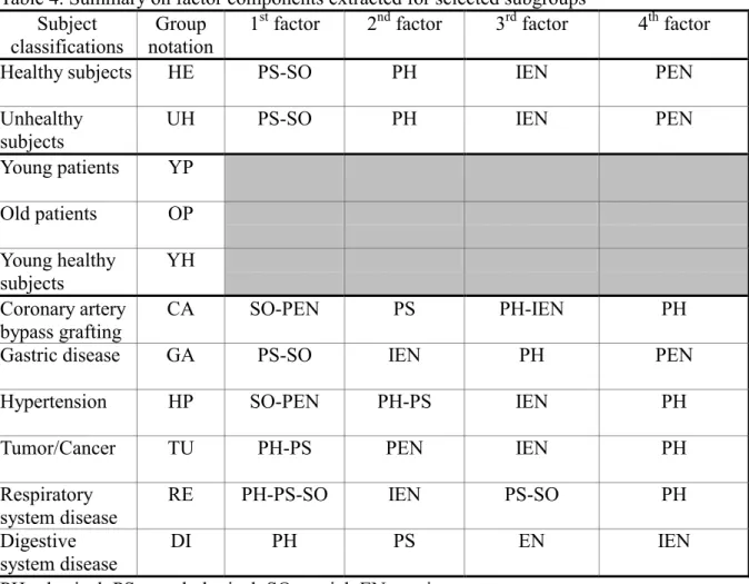
According to the factor patterns of the EFA results(see Table 3a~Table 3g, Table 4), we found that the subgroups may not have the same factor components and the order of the factors extracted were not the same among subgroups, except for the HE-UH pair. Moreover, though the subgroups have similar factor components(e.g., HE and UH subgroups), the degree of similarity between the factors from two
subgroups may not be satisfied. The FCC matrix tells us such story(see the FCC matrix from each of Table 3’s). The values of the FCC indicate the degree of the similarity between factors. Since the values of the FCC in our analyses are mostly below 0.82 and even below 0.68 for the pair of factors from the source subgroup and the target(healthy) subgroup, we realize that the similarity between a corresponding factors from the two subgroups are very poor.
subgroups.
These indicate that samples with different diseases may have different perception on their QOL from the healthy subgroup and from each other. However, if we form an unhealthy subgroup consisting of all patients, we found that healthy subgroup is more similar to unhealthy subgroup than to the individual disease subgroups although the degree of similarity is not satisfied(see the highest FCC for the HE-UH pair). Moreover, note that the order of the extracted factors to some extent reflects the order of the amount of QOL variances explained by the factors. Based on this idea, we found that different subgroups have different order of factors that explain the total QOL variances. For instance, both HE and UH subgroups have the factors ordered as “psycho-sociological(PS-SO)”, “physiological(PH)”, “informative environment (IEN)”, and “physical environment(PEN)”, but the factor order is
“physical-psychological(PH-PS)”, “physical environment(PEN)”, “informative environment(IEN)”, and “physiological(PH)” for the TU subgroup. In other words, the HE and UH subgroups have emphasized much more on psychosocial factor, while the TU subgroup has focused much more on physio-psychological factor.
In CFA, the lower CFI indices of Model A for the pairs of subgroups suggest that most of the models comparing two subgroups do not have good fit, especially for the HE-disease pairs (see Table 5). This indicates that Model A may not be appropriate. If we further examine the four-factor model for individual subgroups, we may find that the four-factor model may not be suitable either. As a result, we would suspect the appropriateness of a four-factor model to be proposed to diverse disease
subgroups. However, the WHO has proposed the four-factor model to the WHOQOL questionnaires. We will further check this issue in the future when we collect more data. The χ2 discrepancies with the corresponding df between Model A, B, and Model B, C suggest that most of the subgroups have totally different perception on their QOL, except for the YP and OP subgroups. For example, theχ2 discrepancy of comparing Model A and Model B for the HE-UH pair is χ2 =421.30 with df=22, which is statistically significant. This result suggests that Model A is a better model than Model B for the HE-UH pair. In order words, the model with no constrains on factor loadings for the two subgroups is more appropriate. This indicates that the HE and UH subgroups not only have different second-order factor loadings but also have different first-order factor loadings. Therefore, we can conclude that they have distinct viewpoints on their QOL. Similarly, we may compare the factor structures from the YP and OP subgroups by applying the same method. We found that the first- and the second-order factor loadings of the two subgroups are equal. This indicates that young patients and old patients have the same factor structures and they have the same perception on their QOL. YP subgroups has different opinion on their QOL from
14
YH subgroup as well. Additionally, we compare each of the six disease subgroups (CA, GA, HP, TU, RE, DI) individually to the healthy subgroup. We found that HE and HP subgroups also have the same first- and the second-order factor loadings but CA and DO subgroups have different opinions from HE subgroups. Moreover, we conducted the multi-sample analysis on the six disease subgroups simultaneously and found that their QOL perception are totally different (see Table 5). We further did the comparisons between each pair of the six disease subgroups. Table 6 illustrates the results. We note that CA-GA, CA-DI, and HP-DI have different perceptions on their QOL. However, TU-GA, TU-RE, TU-DI, GA-RE, and RE-DI have similar QOL perceptions. GA and DI subgroups have the same first-order factor loadings but different second-order factor loadings.
4. Discussion and Conclusion
In this paper, we show that QOL factor structures constructed either by EFA or by CFA can be compared. In the EFA case, factor congruence coefficient (FCC) was calculated between each factor from the target solution and the corresponding factor from the source solution. Larger coefficient represents more similarity between two corresponding factors. Moreover, factor components and order of factors extracted were also compared between two subgroups. The EFA result concludes that no similar QOL perception was found between each disease subgroup and the healthy subgroup, and among different disease subgroups. However, the unhealthy subgroup consisting of all patients from our first study has more similar QOL perception to the healthy subgroup although the degree of similarity is not very high. This is probably because combination of all diseases may suppress the features of individual diseases. This result manifests that it is necessary to analyze diseases individually for
comparing their factor structures and then making appropriate decision on health service and health resource distribution.
In the CFA case, model comparisons provide us the information on the similarity of factor structures among subgroups. The CFA basically confirms the EFA result. All the discrepancies of the χ2 values between models for pair of subgroups suggest that the QOL perceptions are different among the subgroups, except for the young and old patients and for the healthy subjects and hypertension patients. We can conclude that in general the subjects with different features have different appreciation on their QOL. In the CFA of this study, we constrained all the first- or the second-order factor loadings all in one within models. To make more detailed comparisons on the differences of factor structures among subgroups, we will constrain factor loadings one-by-one to see where and to what extent the differences can be found among subgroups. Moreover, multi-sample analyses can be applied to more than two
groups. Therefore, we will conduct the same method to compare more than two subgroups simultaneously.
This is a pilot quantitative study on the comparisons of factor structures among disease subgroups. In this study, one of the subgroups (i.e., CA subjects) may not be representative and the sample sizes of the subjects with diverse diseases are small. However, these limitations do not eliminate the value of this study. Our purpose is to show that quantitative comparisons on latent structures among diseases are available and the results are meaningful. Consequently, we have more confidence on doing further studies. According to the regulations of the WHO, the WHOQOL-Taiwan group has the responsibility on providing technical supports to those who use the WHOQOL-BREF questionnaire-Taiwan version. Moreover, the researchers who use this questionnaire has the responsibility to provide the WHOQOL-Taiwan group the data they collected in order to construct a large data bank for investigating nationwide norms. Since this questionnaire is recently distributed to a wide range of disease subgroups in the hospitals over Taiwan, we expect to collect more data later. Once we have larger samples on disease subgroups, we will conduct the same statistical
procedures presented in this study to compare the latent QOL structures of the patients with diverse diseases in detail. We expect to specify where and to what extent the differences are among these patients.
References
Bentler, P. M. (1993). EQS structural equations program manual. Los Angeles, CA: BMDP Statistical Software.
Chan, W., Ho, R. M., Leung, K., Chan, D. K. S., & Yung, Y. F. (1999). An alternative
method for evaluating congruence coefficients with procrustes rotation: A bootstrap procedure. Psychological Methods, 4, 378-402.
Gotsuch, R. L. (1983). Factor analysis (2nd ed.). Hillsale, NJ: Lawrence Erlbaum Associates.
Harman, H. H. (1976). Modern factor analysis. Vhicago: the University of Chicago Press.
Joreskog, K. G. (1971). Simultaneous factor analysis in several populations. Psychometrika, 57, 409-426.
16
Joreskog
& D. Sorbom: Advances in factor analysis and structural equation models. Cambridge, Mass: Abt Books.
Joreskog, K. G., & Sorbom, D. (1993). LISREL 8: Structural equation modeling with the
SIMPLIS command language. Hillsdale, NJ: Lawrence Erlbaum Associates. Korth, B., & Tucker, L. R. (1975). The distribution of chance congruence coefficients from simulated data. Psychometrika, 40, 361-372.
Leung, K. F., Tay, M, Cheng, S. W., & Lin, F.(1997): Hong Kong Chinese version World Health Organization quality of life measure—abbreviated version. (WHOQOL-BREF(HK)).
MacCallum, R. C., Widaman, K. F., Zhang, S., & Hong S. (1999). Sample size in factor
analysis. Psychological Methods, 4, 84-99.
Mulaik, S. A. (1972). The foundations of factor analysis. New York: McGraw-Hill. Spearman, C. (1904). General intelligence, objectively determined and measured. American Journal of Psychology, 15, 201-293.
Spearman, C. (1927). The abilities of man. New York: Macmillan.
Szabo, S. (1996). Chap 36: The World Health Organization Quality of Life (WHOQOL) assessment instrument. In B. Spiker (ed.) Quality of life and pharmacoeconomics in clinical trials. (pp.355-362)Philadelphia: Lippincott-Raven.
The WHOQOL Group (1994). Development of the WHOQOL: Rationale and current status. International. Journal of. Mental Health, 23(3), 24-56. The WHOQOL Group (1995). The World Health Organization Quality of Life assessment (WHOQOL): Position paper from the World Health
Organization. Social Science Medicine, 41(10), 1403-1409.
The WHOQOL Group (1998a). The World Health Organization Quality of Life assessment (WHOQOL): Development and general psychometric
properties. Social Science Medicine, 46(12), 1569-1585.
The WHOQOL Group (1998b). Development of the World Health Organization WHOQOL-BREF quality of life assessment. Psychological Medicine, 28, 551-558.
The WHOQOL-Taiwan Group (1999). The User’s manual of the development of the WHOQOL-100 Taiwan version. First Ed.
World Health Organization (1993). WHOQOL study protocol. Geneva: WHO (MNH/PSF/93.9).
19
Table 1 The structure of the standard WHOQOL-100 questionnaire
Domain I—Physical domain
F1.Pain and discomfort F2.Energy and fatigue F3.Sleep and rest
Domain II—Psychological domain
F4.Positive feelings
F5.Thinking, learning, memory, and concentration F6.Self-esteem
F7.Bodily image and appearance F8.Negative feelings
Domain III—Level of independence
F9.Mobility
F10.Activities of daily living
F11.Dependence on medical substances and medical aids F12.Work capacity
Domain IV—Social relationships
F13.Personal relationships F14.Practical social support
F15.Sexual activity Domain V—Environment
F16.Freedom, physical safety, and security F17.Home environment
F18.Financial resources
F19.Health and social care: accessibility and quality
F20.Opportunities for acquiring new information and skills F21.Participation in and opportunities for recreation/leisure Activities
F22.Physical environment:(pollution/noise/traffic/climate) F23.Transport
Table 2. Demographic data of the subgroups
Subject
classifications notation Group N (M:F) Sex*
Age* (mean±s.d.) (range) Healthy subjects HE 214 96:116 37.62±12.42 (18~75) Unhealthy subjects UH 854 434:414 42.57±15.22 (17~89) Young patients YP 610 283:326 35.05±9.35 (17~50) Old patients OP 244 151:88 62.28±8.51 (51~89) Young healthy subjects YH 179 78:100 37.76±9.11 (18~50) coronary artery bypass grafting CA 181 157:24 65.3±8.4 (41~82) Gastric disease GA 79 45:34 56.96±13.75 (21~77) Hypertension HP 77 53:24 54.94±13.12 (22~80) Tumor/Cancer TU 63 27:36 48.00±12.25 (23~75) Respiratory system disease RE 61 34:27 38.43±11.69 (18~70) Digestive system Disease DI 60 44:16 45.57±13.43 (21~72) * Missing data are excluded for this variable.
21
Table 3b. Unhealthy (UH) subgroups
F1 F2 F3 F4 Pain -0.04 0.37 -0.03 0.12 Energy 0.03 0.47 0.16 0.18 Sleep -0.08 0.46 0.09 0.20 Mobil 0.25 0.40 0.15 -0.22 Activ 0.49 0.30 0.10 -0.05 Medic 0.03 0.60 -0.14 0.00 Work 0.51 0.33 0.02 -0.20 Pfeel 0.05 0.15 0.28 0.07 Think 0.28 0.16 0.12 0.03 Esteem 0.50 0.20 -0.03 0.19 Body 0.42 0.17 0.04 -0.01 Neg 0.14 0.23 -0.06 0.28 Spirit 0.40 0.10 0.18 -0.03 Relat 0.77 -0.07 -0.11 0.11 Supp 0.64 -0.16 0.07 0.07 Sex 0.51 0.11 -0.12 0.09 Safty 0.16 0.20 0.03 0.32 Home 0.32 -0.03 0.11 0.41 Finan -0.06 0.04 0.51 0.18 Servic 0.23 -0.22 0.34 0.15 Inform 0.03 -0.07 0.69 -0.08 Leisur -0.03 0.19 0.47 0.09 Envir -0.03 0.06 -0.01 0.54 Transp 0.06 0.02 0.10 0.42 Respect 0.47 -0.05 0.20 0.12 Eating 0.23 0.13 0.21 0.07 % variance explained 24.7% 17.0% 18.7% 11.5% Factor Coeff. Congruence
UH: F1 UH: F2 UH: F3 UH: F4
HE: F1 0.876 0.326 0.259 0.178
HE: F2 0.345 0.652 0.439 0.215
HE: F3 0.205 0.190 0.714 0.347
HE: F4 0.103 0.085 0.160 0.846
root-mean square deviation
UH: F1 UH: F2 UH: F3 UH: F4
HE: F1 0.165 0.337 0.345 0.351
HE: F2 0.366 0.233 0.287 0.325
HE: F3 0.371 0.311 0.178 0.256
Table 4. Summary on factor components extracted for selected subgroups Subject
classifications
Group notation
1st factor 2nd factor 3rd factor 4th factor
Healthy subjects HE PS-SO PH IEN PEN
Unhealthy subjects
UH PS-SO PH IEN PEN
Young patients YP Old patients OP Young healthy subjects YH Coronary artery bypass grafting CA SO-PEN PS PH-IEN PH
Gastric disease GA PS-SO IEN PH PEN
Hypertension HP SO-PEN PH-PS IEN PH
Tumor/Cancer TU PH-PS PEN IEN PH
Respiratory system disease
RE PH-PS-SO IEN PS-SO PH
Digestive system disease
DI PH PS EN IEN
PH=physical, PS=psychological, SO=social, EN=environment, PEN=physical environment, IEN=informative environment
23
Table 5. The χ2, degree of freedom (df), and the CFI index for Model A, B, C on selected pairs of the subgroups Between two subgroups:
groups HE(n=214) UH(n=854) YP(n=610) OP(n=244) YH(n=179)
HE (n=214) A:1149.70,df=590;0.874 B:1571.00,df=612;0.869 C:1584.61,df=616;0.868 UH (n=854) YP (n=610) A:1266.73,df=590;0.886 B:1298.85;df=612;0.884 C:1305.75,df=616;0.883 A:1187.27,df=590;0.888 B:1230.00,df=612;0.884 C:1239.97,df=616;0.883 OP (n=244) YH (n=179)
groups CA(n=181) GA(n=79) HP(n=77) TU(n=63) RE(n=61) DI(n=60)
HE (n=214) A:1149.70,df=590;0.827 B:1218.99,df=612;0.813 C:1237.94,df=616;0.808 A: 987.24,df=590;0.813 B:1025.01,df=612;0.806 C:1030.07,df=616;0.805 A:1042.93,df=590;0.793 B:1069.29,df=612;0.791 C:1073.19,df=616;0.791 A:1015.30,df=590;0.788 B:1070.86,df=612;0.771 C:1075.06,df=616;0.771 A: 989.39,df=590;0.800 B:1032.85,df=612;0.789 C:1042.02,df=616;0.786 A: 968.96,df=590;0.799 B:1018.47,df=612;0.784 C:1038.68,df=616;0.775 Among six disease subgroups:
A:2711.50,df=1770;0.793 B:2889.16,df=1880;0.778 C:2940.01,df=1900;0.771
Table 6. The χ2(1st value), degree of freedom(2nd value), and the CFI index (3rd value)for Model A, B, C:
CA(n=181) TU(n=63) HP(n=77) GA(n=79) RE(n=61) DI(n=60) CA (n=181) A:1017.66,df=590;0.813 B:1060.41,df=612;0.804 C:1061.65,df=616;0.805 A:1045.29,df=590;0.815 B:1087.34,df=612;0.807 C:1095.74,df=616;0.805 A: 989.60,df=590;0.834 B:1029.96,df=612;0.826 C:1046.93,df=616;0.821 A: 991.75,df=590;0.823 B:1037.36,df=612;0.813 C:1045.03,df=616;0.811 A: 971.32,df=590;0.824 B:1008.19,df=612;0.817 C:1036.24,df=616;0.806 TU (n=63) A: 910.90,df=590;0.739 B: 963.41,df=612;0.714 C: 964.47,df=616;0.716 A: 855.20,df=590;0.774 B: 870.71,df=612;0.779 C: 875.59,df=616;0.778 A: 857.35,df=590;0.742 B: 876.90,df=612;0.744 C: 879.23,df=616;0.746 A: 836.92,df=590;0.733 B: 855.38,df=612;0.737 C: 868.95,df=616;0.727 HP (n=77) A: 882.83,df=590;0.783 B: 921.63,df=612;0.771 C: 927.60,df=616;0.769 A: 884.98,df=590;0.757 B: 930.74,df=612;0.738 C: 934.69,df=616;0.738 A: 864.55,df=590;0.752 B: 899.54,df=612;0.740 C: 912.05,df=616;0.732 GA (n=79) A: 829.29,df=590;0.793 B: 849.22,df=612;0.795 C: 854.20,df=616;0.794 A: 808.86,df=590;0.791 B: 823.68,df=612;0.798 C: 836.21,df=616;0.790 RE (n=61) A: 811.01,df=590;0.758 B: 835.86,df=612;0.755 C: 842.85,df=616;0.751 DI (n=60)
RED:A-B & B-C are not statistically significant.
YELLOW:A-B is not statistically significant,but B-C is statistically significant
BLUE:A-B is statistically significant,but B-C is not statistically significant
WHITE:A-B & B-C are statistically significant.
Critical values:χ2 (α=0.05, df=22)=33.93 χ2 (α=0.05, df=4) =9.49
Can We, Who Should, and How to Weight
the Dimensions of Quality of Life Measures?
I. Introduction
A measure of Health-related quality of life (HROQOL) contains many dimensions. For example, the WHOQOL questionnaire is composed of six domains: physical, psychological, independence level, social relationships, environment, spirituality/religion/personal beliefs, or in its short form, the six domains are combined into four main domains: physical, psychological, social relationship, and environment. In any case, under the domain level, there are many facets (or sub-domains). Within each facet, there are many items. When researchers score subject’s QOL score, they may directly sum item scores to obtain facet score, and sum facet scores to obtain domain score. In addition, in some QOL measures, researchers may directly sum the domain scores to obtain an overall QOL score. For this simple summation approach, assigning equal weights on items/facets/domains is the most common method. In other words, researchers assume that subject gives equal importance on each item/fact/domain. As a result, subject’s overall QOL score is simply the summation of all items/facets/domains. This approach is quite intuitive and conceptually and arithmetically simple, however, this approach has been inquired recently (Perloff & Persons, 1988). One of the arguments is that different QOL domains as well as facets and items may have different meanings to individuals in terms of relative importance (Bowling, 1997; Streiner & Norman, 1989). As a result, equal weighting approach may underestimate the QOL dimensions/facets/items with more importance and overestimate the QOL dimensions/facets/items with less importance to individuals. Furthermore, direct summation approach may erroneously converts what is at best ordinal data into interval levels of measurement (Bowling, 1997). Therefore, statistical caution is required. Although, a total score is better to be used than separate sub-scores, we should realize that a given total score can be arrived in different ways. This implies that subjects with the same total scores may not have the same QOL. Moreover, if the number of the item (or facet) within a facet (or domain) is larger, simple summation method may lead to obtaining more weight or contribution for this facet (or domain) to overall QOL score. This may not be reasonable because larger number of the items (facets) indicates only wider-coverage but not more importance to overall QOL score. Considering all the problems of direct summation approach, the alternative is to assign different values (weights) to different items/facets/domains for scoring purpose. Therefore, some researchers have started
to study how to give appropriate weights to different domains as well as facets and items so that the overall QOL score can be more appropriate to represent individual true QOL (Lei & Skinner, 1980; Perloff & Persons, 1988; Wainer, 1976).
The purpose of this exploratory study attempts to find the more appropriate ways to weigh the dimensions of QOL measures so that the assessment of QOL can describe subject’ true QOL level better and the overall QOL score is much more meaningful. Three main questions should be discussed in this study. First, “CAN we give weights?” Is it reasonable to sum domain (as well as facet and item) scores to form an overall QOL score? Can we do it without any assumptions or under certain conditions? Second, “WHO should give the weights?” Should it be the health service users, the health service providers, the health policy makers, or the public? Third, “HOW to weight the dimensions?” Should we use regression approach, factor analysis approach, multi-attribute utility approach, or direct rating? Is there any optimal method? In this study, we will explore these questions.
II. Can we give weights?
This question involves a methodological and philosophical issue. To answer this question, we should first make clarification on the meanings of “overall QOL score”, “domain score” and “facet score”. Usually researchers design several homogeneous items with the same properties to measure a facet. As a result, a facet score is obtained directly by summing all the item scores in the same facet. Moreover, several facets with the same properties, if this is true, may be designed to measure a domain. Consequently, a domain score is obtained by summing all the facet scores in the same domain. Note that all items within a facet have the same properties (i.e., homogeneity) and all facets within a domain have the same properties as well. Therefore, it is reasonable to sum all homogeneous item scores to obtain a facet score and sum all homogeneous facet scores to obtain a domain score. However, we cannot say that all domains under a big QOL concept have the same properties so that we can sum all domain scores to form an overall QOL score unless we make certain assumptions. This is because different (heterogeneous) domains are different perspectives of the QOL concept. It is not reasonable to sum the heterogeneous domain scores that have different properties. The analogy just likes we sum the scores of sweetness, color, and odor of an apple to form a total score. What is the meaning of this total score? In the past, many studies discussed if it is reasonable to use Likert summated scale method, that is, simple summation method by adding all item scores to form a total score. For this summation approach, two assumptions should be made (Fayers & Machin, 1998): 1. Each item can be scored on a simple linear scale (e.g., 1 to 5) and the scale has the
total score.
2. Each item is measuring the same attribute, therefore, direct summation does not cause any problem.
According the perspectives of Fayers & Machin, the properties of “equal interval” and “homogeneity” become the criteria for evaluating the possibility of simple summation.
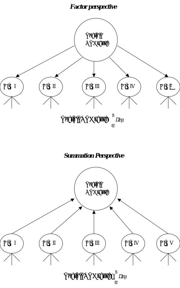
On the other hand, if we can define that the overall QOL score is just the composition of all domain scores then we can do direct summation. Therefore, to answer this question we should first find that how we define the “overall QOL score” as well as “domain score” and “facet score”. Figure 1 shows two perspectives on forming total QOL score. Note that the directions of the arrows in the two perspectives are different. The first one—“factor perspective” does not allow us to sum domain scores to form an overall QOL score, however, the second theory—“summation perspective” allows us to do so. These are two totally different philosophies on the definition of research question. Perloff and Persons (1988) also mentioned that whether we can “add apples and oranges”, it all depends on the research question to be asked/defined. Although, we may find some researchers do not suggest people to directly sum different dimension scores to form an overall score (WHO, 1995), we still can find many psychological and clinical measures apply this approach to obtain subject’s overall score on a measure. One of the advantages of this direct summation approach is that a single (overall) score can be obtained so that it is easier to make comparisons among subjects. Suppose we can only obtain six domain scores but not an overall QOL score, it will be very hard to say whether a subject has a better QOL than others. In summary, we need to be very careful when we apply this direct summation approach. We need to clearly define the meaning of the overall QOL score in our study.
Wright and Feinstein (1992) looked at the discrepancies between factor and summation perspectives from the viewpoint of “psychometrics vs. clinimetrics”. Psychometrics is a quantitative methodology for psychologist. Clinimetrics is a quantitative methodology for clinicians. They addressed that both methods have different concepts and goals, and then apply different measurement principles. Psychological measurement focuses on people’s attitude, opinions, and interpersonal relationships which are more subjective. However, clinical measurement focuses on people’s physical condition and functions which are more objective. As a result, psychometricians design many homogeneous items to measure an attribute so that summing the homogeneous item scores to form an index for an attribute is appropriate but it is not appropriate to sum items from heterogeneous attributes. On the other hand, clinimetricians use to aggregate multiattribute (heterogeneous) scores to form an
index (e.g., APGAR score). Consequently, internal reliability (e.g., internal consistency) is important in psychometric measurement. Several special statistical tests are conducted to test the reliability of the psychological measures. On the other hand, clinicians always aim their strategies at choosing the most important attributes to be included in the index no matter if the attributes are heterogeneous. Therefore, consensus from all clinicians is important in clinimetric measurement.
Coste, Fermanian, and Venot (1995) surveyed six major medical and
epidemiological journals from 1988 to 1992. They found that most of the composite measurement scales used in the medical literature were lack of measurement
properties such as (content, criterion, and construct) validity, and (inter-observer, intra-observer, and test-retest) reliability. In addition, item selection, item validation, and appropriate multivariate statistical analysis methods were also missing. This
implies that many health-related composite scales are invalid. Therefore, as the psychometricians we suggest to use the psychmetrician’s viewpoints. This is because QOL measurement is a more subjective judgment. Subjects’ opinions and attitudes toward their experience in their personal life are investigated. Moreover, a
measurement scale developed from the viewpoints of psychometricians is more reliable and valid in terms of research methodology.
III. Who should give weights?
To answer this question, we should focus on the purpose of the QOL measurement. What’s the final usage of this QOL score? What are the assumptions to answer this question? If this score is measured only for understanding an individual’s subjective QOL feeling, data collected from individuals are enough. Carr and his colleagues (Carr, 1996; Carr & Higginson, 2001) even addressed the importance of patient-centered QOL measurement. They proposed not only individual definition of QOL but also individual weightings on different QOL dimensions for each patient. They mentioned that a true QOL assessment can only be achieved by using weights from individual patients. We may not agree with all their opinions but we should not ignore the importance of individual’s viewpoints on his/her QOL. Several studies show that many current QOL measures do not include the dimensions that are important to patients and the public (Bowling, 1997; Carr & Higginson, 2001). The discrepancies between the existing instruments and people’s opinions on the dimensions to be considered in a QOL measure should be minimized. Past studies show that under most conditions, individual is the best person to present his/her own QOL subjective feeling. Moreover, many studies show that patient’s caregivers and even his/her medical care professionals may either underestimate or overestimate patient’s QOL perceptions to diverse extents which depend on the traits that QOL
measurement attempts to assess (Addinbton-Hall & Kalra, 2001; Kwoh, O’Connor, Regan-Smith, Olmstead, Brown, Burnett, Hochman, King, & Morgan, 1992; Pearlman & Uhlmann, 1988; Slevin, Plant, Lynch, Drinkwater, Gregory, 1988; Wilson, Dowling, Abdolell & Tannock, 2000). However, in some situations such as patients with cognitive impairments, communication deficits, severe distress caused by their symptoms or physical or emotional burdens toward the QOL measure, the proxy (e.g., his/her caregivers) may be a better alternative to answer the QOL questionnaire (Addinbton-Hall & Kalra, 2001). Addinbton-Hall and Kalra (2001) provided a good review on “Who should measure quality of life?”— which discusses the factors affecting agreement in QOL assessment by patient, his/her proxy, and doctors.
If medical decisions, such as clinical treatment evaluation and intervention, are the final purpose, both patients’ and medical professionals’ opinions are important. Physicians can choose whatever the better treatments that they think for patients under patients’ consents and cooperation so that the treatment benefits can be maximized. Opinions from policy-makers are important too when making medical policies as well as social resource allocation. They not only have legislative power to make important public decisions but also assumedly have social justice and understanding on social resources and people’s needs so that they can make more appropriate decisions. In addition, the voices from the public cannot be neglected too when making public medical decisions such as the allocation of medical expenses. This is because social resources are from the public and should be used in the public. As a result, when making social resource allocation such as in Taiwan’s National Health Insurance(全 民健保), the opinions from policy-makers, the public, medical professions, and patients should be comprehensively considered. In summary, to answer “Who should give the weights?” is a very difficult task and its answer depends on the purpose of the QOL measures to be used. It seems that we cannot find an optimal way to answer this question. However, we should ask all the policy decision-makers to make their decisions as optimal as possible. We suggest that all the policy decision-makers should not only consider social fairness and justice but also consider individual’s benefits so that better public decisions can be made and the needs of the minority (such as the poor, the disabled, and the elders) are not neglected.
Table 1 presents the four possible persons to give weights on domains/facets/items of QOL measures. In this table, the assumptions, the advantages, and the disadvantages of using each person’s weighting are illustrated. For example, to estimate patient’s subjective QOL level, the best way is to collect data directly from the patient. Moreover, patient’s opinion is also important in selecting appropriate treatment from several available treatments provided by his/her physician. However, patient’s opinion may be too personalized so that it is not applicable to policy-making.
To use patient’s weighting opinion as a standard, one assumption should be made: patients with the same disease and at the same disease stage have stable and consistent judgment; moreover, patient keeps the same judgment during entire disease periods (Staquet, Hays, & Fayers, 1998). Policy-makers’ opinions are important for making medical policies and social resource allocation; however, they may neglect individual’s needs. As a result, the needs of the minority may be ignored. Therefore, good policy-makes should have social justice and kindly mind. They should not only know how to allocate medical resources fairly but also know how to fulfill individual’s needs, especially for the weak and the poor.
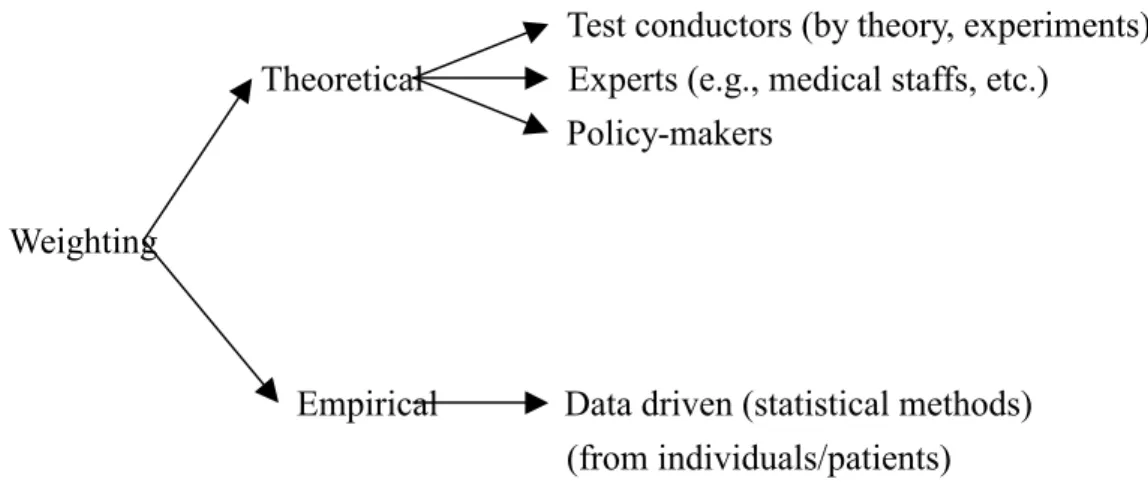
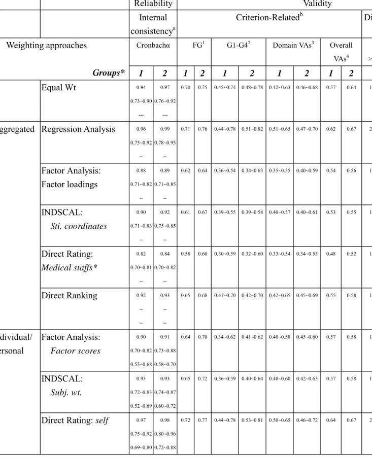
The first column in Table 1 shows that the four possible persons of giving weights can be classified into 3 groups according to how QOL weights can be obtained. Policy-makers and the public are classified into the aggregated weighting group. Since it is not practical for them to give different weights on the different dimensions for different individuals. Their weighting opinions are usually aggregated to form a set of weighting values to represent general importance of QOL domains. For example, mean rating can be calculated based on their opinions. On the other hand, patient’s opinion is classified into individual or personal weighting group. This is because by some direct and/or statistical methods we can collect individual’s weighting on each item/facet/domain along with his/her subjective QOL measures. In other words, information on both importance weighting and subjective feeling on different QOL domains for individual can be obtained. Mozes and Shabtai (1996) did collected QOL dimension scores and personal ratings on the importance of each dimension in a QOL measure to study how to weight the diverse QOL dimensions. Medical professionals’ opinions on weighting dimensions lie in between the two weighting groups. They may give a set of weights to their patients individually. They may also just give a general (averaged) set of weights according to their experience. For the latter case, mean weighting should be calculated to obtain a set of weighting values. The advantage of individual/personal weighting approach is that we can obtain different weighting sets for different individuals so that the overall QOL scores may be more representative to individuals. Carr and Higginson (2001) pointed out that a true assessment of QOL can only be achieved using weights for individual patients. However, the disadvantage is that their weighting opinions may not reflect population’s opinions. Moreover, it is not easy to collect individual’s opinion from enough and representative samples. Therefore, it has its limits on applications in general. On the other hand, the advantage of the aggregated weighting approach is that the result is more appropriate to be used in social resource allocation.
The main purpose of this paper is to find simpler ways (i.e., sets of weights) to summarize a set of items/facets/domains so that a better overall QOL index can be obtained. Two general types of weighting approaches can be considered: theoretical and empirical (see Figure 2). Theoretical type refers to assigning a set of weights to the dimensions of a scale by the test constructor. They may be based on their understandings on the scale, they may consider experts’ opinions (such as doctors’), or they may even conduct experiments to obtain weights. It is a more intuitive type of approach in assigning weights. The aggregated weighting group mentioned above may be considered as this type of approach because a set of averaged weights is calculated from a specific group such as medical experts. Empirical type refers to obtaining weights by statistical data analysis such as regression, factor analysis, etc. Usually, the raw data are collected from patients. The individual weighting group mentioned above may be considered as this type of approach because individual weighting can be obtained. According to the past studies and our propositions, we summarize the following possible statistical weighting approaches.
1. Regression Approach:
This approach is a very common approach that uses ordinary regression method to obtain (standardized) regression coefficients as the base of weights for different QOL dimensions (Levine, Halberstadt, & Goldstone, 1996; Perloff & Persons, 1988; Rose, Scholler, Klapp, & Bernheirn, 1998; Staquet, Hays, & Fayers, 1998; Streiner & Norman, 1989). Usually, researchers use different dimension/facet/item scores as the independent/predictor variables (Xs’) and a criterion score as the dependent variable (Y). The criterion score may be an external overall QOL score. The regression equation is as follows:
k kX b X b X b b Yˆ = 0 + 1 1+ 2 2 +...+ .
whereYˆ is the predicted Y; b0 is the intercept and bis’ (i=1,…,k) are the regression
coefficients. An optimal set of regression coefficients is searched to maximize the predictive accuracy of the equation. This regression approach can be considered to define a weighting scheme for individual dimension/facet/item to improve the predictive accuracy of the dependent variable. Perloff and Persons (1988) did prove that arbitrary weighted index (usually equal-weighted) results in biased on prediction but weighting by multiple regression approach can significantly improve the predictive ability of an index. They presented three tests for detecting the bias and showed how an unbiased weights can be calculated especially by using multiple regression. In practice, researchers often use standardized regression form. The standardized regression equation is the following form:
k X k X X Y Z Z Z Zˆ =β +β +β +...+β 2 1 2 1 0
whereZˆ is the predicted standardized Y;Y
i
X
Z s’ are the standardized X scores i
(i=1,…,k); β0 is a constant (in standardized regression form, β0=0) and β1,…, βk are
the ‘beta weights” for the k dimensions/facets/items. The reasons that researchers use standardized regression form but not non-standardized regression form are that standardized regression approach allows us to adjust unequal scales among the predictor variables and therefore make cross comparisons available. As a result, the standardized regression coefficients imply the relative importance of different QOL dimensions/ facets/items to a more accurate extent. A total QOL score is equal to the summation of standardized regression coefficients multiplying their corresponding dimensions/ facets/items. Although, this approach is more difficult than direct rating/weighting (see the following discussion) approach and it increases computation complexity, modern computer and statistical package can help us to do a great job.
2. Multivariate Approaches:
Multivariate approaches such as exploratory factor analysis (EFA), multidimensional scaling (MDS), and cluster analysis (CA) can be considered to use in the weighting task. For example, Ki and Chow (1995) applied EFA with principal component analysis to summarize 11 subscales of a QOL measure in three factors. Each subscale has loading (i.e., weight) on each of the three independent factors. EFA is a data reduction technique that can simplify many variables in terms of smaller number of factors. Therefore, the number of factors may be less than what we expected (e.g., in the WHOQOL questionnaire, we expected the number is six for domains). In some studies, factor scores derived from factor analysis solution may be used as the weights for individuals (Olschewski & Schumacher, 1990); however, recently psychometricians do not suggest to do so because factor scores are often neither very precise nor uniquely defined (Fayers & Machin, 1998; Krzanowski, 1988). Although we may find that many studies used factor analysis to obtain weights on items/facets/domains, Kaplan (1998) did not suggest to do so because he thought that factor analysis solution and relative importance on dimensions are conceptually and empirically independent. Factor analysis solution (e.g., factor loadings) reflects the correlations of variables to factors extracted but not the relative importances among variables.
In addition, one of the MDS models (i.e., the INDSCAL, INdividual Difference SCALing model) allows us to differentiate not only intraindividual variation but also interindividual differences in perception. As a result, subjects’ relative importance on dimensions can be estimated. The INDSCAL (Arabie, Carroll, &
DeSarbo, 1987; Carroll, 1972; Carroll & Chang, 1970; Carroll & Wish, 1974a, 1974b; Wish & Carroll, 1974) explicitly generates individual differences on the weights or perceptual importances of dimensions. The central assumption of this model is the definition of distances for different individuals. Mathematically, we can express the distance between stimuli j and k for subject i as djk(i) where
(
)
2 1 ] [ 1 2 ) (∑
= − = R r kr jr ir i jk w x x dwhere R is the dimensionality of stimulus space, xjr is the coordinate of stimulus j
on the rth dimension of the group stimulus space, and wir is the weight (indicating
salience or perceptual importance) of the rth dimension for the ith subject. The
input data for the INDSCAL is a matrix of proximity (or antiproximity), the general
entry of which is the dissimilarity of stimuli j and k for subject i (i.e., δjk(i)). For n
stimuli and I subjects, this size of the input matrix is n x n x I. The output consists of two matrices (see Figure 3), one is an n x R matrix, X=( xjr) of stimulus
coordinates, another matrix is an I x R matrix, W=(wir) of subject weights. One
important property of INDSCAL is that its recovered dimensions are unique, that is, it is not subject to the rotational indeterminacy (Carroll & Arabie, 1998). In the psychological model, the dimensions are supposed to correspond to fundamental perceptual or other process whose strengths, sensitivities, or importances vary among individuals. In practice, suppose we can estimate the correlation matrix C
among all variables (i.e., items/facets/ domains) of a QOL measure for individual. Then the input data matrix for individual on the INDSCAL is a matrix of [I-C], that
is, a matrix of dissimilarity. As the EFA, the number of dimensionality R may be less than what we expected. This indicates that the MDS provides a data reduction solution as in EFA and CA. In practice, many studies use MDS approach to estimate the weights for different dimensions and individual’s weights on different dimensions; however, we should realize that the MDS study design has to be very careful (Gabrielsson, 1973; Gromko, 1993; Kalberstadt & Niedenthal, 1997; Morley & Pallin, 1995; Schiffman, Musante, & Conger, 1978; Sherman & Ross, 1972; West, 1986). In other words, repeated measures (or instead, homogeneous items in the same facet in the QOL scale) should be collected for the variables for each individual so that the correlation matrix (the input data matrix) among all variables can be obtained for each individual.
3. Utility Approach:
Utility approach is one of the most popular approaches on assessing subject’s QOL. This approach is based on economic theory. Consequently, its result (usually its score ranges from 0 to 1) can be used in medical decision-making such as social
resource allocation. Three most common utility methods are rating scale (RS), standard gamble (SG), and time trade-off (TTO) which will be explained later. There are some extensions based on this approach. Economists attempted to derive a numerical value to a health state. The most well-known index is quality- adjusted life year (QALY). The original purpose of QALYs is for cost-effectiveness analysis so that social cost of illness can be estimated and medical resource can be allocated (Brooks, 1996; Schwartz & Laitin, 1998). QALYs combine both length (quantity) and quality of life into one single index (Brooks, 1996; Bowling, 1997). Quantity of life indicates life expectancy or life year. Quality of life is usually estimated by utility methods such as standard gamble, time trade-off, rating scale, etc. The utility method comes out a score between 0 (dead) and 1 (perfect health). QOL estimation employs a set of weights to quality-adjust these life years. As a result, a QALY can be considered as weighted life length by using quality of life. The advantages of QALY are that it allows the comparisons among different treatments and among the outcome of different sectors in health care. On the other hand, Hwang and Wang (2001) adapted the approach and developed survival weighted psychometric assessment for health-related quality of life. Their approach takes survival rate into account so that better QOL can be estimated. As a result, their QOL measure can be considered as a weighted QOL by using survival probability.
Moreover, multi-attribute utility approach is a method of assigning an overall utility score to a given health state while specially assessing the contribution of each significant component/dimension/attribute of overall health (Jansen,
Stiggelbout, Nooij, & Kievit, 2000). It integrates subjective judgment on individual components and then comes out an overall utility score. Torrance, Feeny, Furlong, Barr, Zhang, and Wang (1996) provided an alternative multiattribute utility
approach so that the utilities for individual attributes can be obtained first. Then general multiplicative formulas are applied to obtained overall utility as an aggregation of the separate attribute utilities. For example, Jansen, Stiggelbout, Nooij, and Kievit (2000) calculated multiattribute utility score for r attributes as
∑
= r i ih ihs w 1 .where wih=the importance weight (0-1) for attribute i for subject h; sih=the health
status attribute score (0-1) for attribute i for subject h. This is a weighted attribute score in which the importance weighting score is first obtained by using a 0(not important) ~100(very important) rating scale on each attribute according to subject’s importance. The importance ratings are then transformed into ratio weights, for each subject, by dividing the rating of each attribute by the sum of all ratings. As a result, individual ratio weights for each attribute are summed to one.