即時無線瞌睡偵測腦機介面系統

(1)

國立交通大學

電機與控制工程學系

碩士論文

即時無線瞌睡偵測腦機介面系統

Real-time Wireless Brain Computer Interface for

Drowsiness Detection

研究生：張哲睿

指導教授：林進燈博士

中華民國九十八年七月

(2)

即時無線瞌睡偵測腦機介面系統

Real-time Wireless Brain Computer Interface for Drowsiness

Detection

研究生：張哲睿 Student：Che-Jui Chang

指導教授：林進燈博士

Advisor：Dr. Chin-Teng Lin

國立交通大學

電機與控制工程學系

碩士論文

A Thesis

Submitted to Department of Electrical and Control Engineering

College of Electrical Engineering

National Chiao Tung University

in Partial Fulfillment of the Requirements

for the Degree of Master

in

Electrical and Control Engineering

July 2009

Hsinchu, Taiwan, Republic of China

(3)

即時無線瞌睡偵測腦機介面系統

學生：張哲睿

指導教授：林進燈博士

國立交通大學電機與控制工程研究所

摘要

近年來，交通意外是一個造成駕駛死亡的至關重要原因，其中駕駛者的精神狀況不佳所造成車禍意外佔了絕大多數比例，所以開車駕駛瞌睡監控問題是我們嘗試克服之處，試著以人為方式來減少車禍發生。近年來相關的開車監控研究主要著重在使用者影像辨識上，瞳孔辨識、眨眼辨識或是偵測司機擺頭頻率，但是，這些影像相關研究存在著先天上的缺點，使用者必須正對鏡頭才能得到好的量測結果；此外為了克服此點，其他學者引進了生理參數來做為開車即時瞌睡狀況的比較依據，如心電圖、眼電圖、肌電圖或腦波圖等，較影像辨識來得直接與精確，使用者可以不必受影像定位之問題影響，本論文即對於此生理參數中腦波參數做進一步的探討，並且設計一套無線可攜式的腦波擷取系統與數位訊號處理平台並且搭配非監督式分析演算法做即時瞌睡判斷，其優勢在於可移除掉不同人、不同次測量中個別跟環境差異性。本論文藉由虛擬實境模擬環境所記錄下開車偏移量來當作瞌睡程度的參考，並與所發展的非監督式分析法的相互比對關係來證明此演算法對瞌睡程度偵測的功效與可行性，最後實現在數位訊號處理平台上。經由實際測試，可以成功在駕駛者有睡意時，利用聲音警示提醒駕駛保持清醒，確保開車時的安全。

(4)

Real-time Wireless Brain Computer Interface for

Drowsiness Detection

Student: Che-Jui Chang

Advisor: Dr. Chin-Teng Lin

Department of Electrical and Control Engineering

National Chiao Tung University

Abstract

In recent years, traffic accident is one of the critical reasons to cause deaths of drivers. Here, Drivers’ drowsiness has been implicated as a causal factor in many accidents because of the marked decline in drivers’ perception of risk and recognition of danger, and diminished vehicle handling abilities. Therefore, if the mental state of drivers can be real-time monitored directly, drowsiness detection and warning can effectively avoid disasters such as vehicle crashes in working environments. Some previous researches used non-physiological method, as eye closure with CCD image tracking, such as the pupil recognition, blink detection or identification the drivers head shaking frequency. However, for CCD image tracking, users couldn’t move for free, and the images detecting performance were easily be interfered by light. And others used physiological parameters to increase the accuracy of drowsy detection, like pulse wave analysis with neural network, the electrooculogram (EOG) and the electromyography (EMG) measurement, and the electroencephalogram (EEG). In this study, we proposed a real-time wireless brain computer interface for drowsiness

(5)

detection. Here, a small, light, and portable EEG acquisition module was designed for long-time EEG monitoring. And a novel algorithm of drowsiness detection based on was also proposed to reduce the computation complexity, and was implemented in a portable DSP module. In order to estimate the level of drowsiness, a lane-keeping driving experiment was designed. The drowsiness level of drivers was indirectly assessed by the reaction time and driving trajectory under Virtual Reality Driving Simulation Environment. The advantage of this unsupervised algorithm can remove the differences between individual and environment in different people or measurements. In order to verify the accurate and feasibility of our proposed unsupervised algorithm, we compared drowsiness status estimated by driving performance with that obtained by our proposed unsupervised algorithm. The results showed that our proposed algorithm can detect driver’s drowsiness status. Finally, our system can successfully be applied in practice to prevent traffic accidents caused by drowsy driving.

KEYWORD: drowsiness detection, electroencephalogram, portable EEG acquisition module, DSP module, Virtual Reality Driving Simulation Environment,

(6)

誌謝

本論文的完成，首先要感謝指導教授林進燈博士這兩年來的悉心指導，讓我學習到許多寶貴的知識，在學業及研究方法上也受益良多。另外也要感謝口試委員們的建議與指教，使得本論文更為完整。其次，感謝實驗室的學長林伯昰、學長鍾仁峰及學長柯立偉在研究上的指導。同學有德、家欣、介恩、昕展，在過去兩年研究生活中同甘共苦、相互扶持，及學姐真如、依伶與毓婷、學長家達、孟修、煒忠、儀晟、寓鈞與建昇、學弟妹們育航、智賢、璽文、聖翔、佩瑄與佳鈴，在研究過程中所給我的鼓勵與協助，以及碩士班新生智綸、晉澤與琬茹在過去兩個月的幫忙。尤其是家達學長、依伶學姐及伯昰學長，在研究理論及程式技巧上給予我相當多的幫助與建議，亦師亦友，讓我獲益良多。也同樣感謝實驗室助理在許多事務上的幫助。感謝我的父母親對我的教育與栽培，並給予我精神及物質上的一切支援，使我能安心地致力於學業，此外也感謝對我不斷的關心與鼓勵。最後我要感謝我的女朋友佳鈴，在我繁忙之中還有新鮮的水果可以享用，更不時叮嚀我的健康，有妳的陪伴讓我倍感窩心，使我能全心投入論文之中，謝謝你們。謹以本論文獻給我的家人及所有關心我的師長與朋友們。

(7)

List of Tables

Table 2-1: Common band of EEG ...12 Table 3-1: System specification of IA, HP, and LP filter for portable EEG acquisition module...25 Table 3-2: Definition and function for pins of SPI mode ...29 Table 3-3: The spec of portable EEG acquisition module ...42 Table 5-1: The comparison of the correlation between power and driving performance and MD* and driving performance for channel OZ ... 62 Table 5-2: The description of binary classification test ...63 Table 5-3: The results of binary classification test ...70

(10)

List of Figures

Fig. 1-1: The role of driver status monitor [48] ...4

Fig. 1-2: Flowchart of EEG processing in drowsy estimation system [54] ...6

Fig. 1-3: Flowchart of EEG processing in EEG-based drivers’ cognitive states estimation system [55] ...6

Fig. 1-4: Scan NuAmps Express system (Compumedics Ltd., VIC, Australia) ...7

Fig. 2-1: A typical BCI system architecture...10

Fig. 2-2: International 10-20 system...13

Fig. 2-3: The overview of surrounded VR scene.. ...14

Fig. 2-4: The digitized highway scene [61].. ...15

Fig. 2-5: Illustration of synchronization between the driving trajectory and EEG data ...16

Fig. 2-6: Steps of EEG preprocessing...17

Fig. 2-7: Illustration of 8-second moving window with 7-second overlap...17

Fig. 2-8: The flowchart of the EEG analysis method. ...19

Fig. 3-1: Illustration of hardware framework of our BCI system ...21

Fig. 3-2: Block diagram of Portable EEG acquisition module ...22

Fig. 3-3: Circuits of preamplifier ...23

Fig. 3-4: Simulation of preamplifier’s gain response ...23

Fig. 3-5: Circuits of band-pass filter ...24

Fig. 3-6: Simulation of band-pass filter’s gain response ...24

Fig. 3-7: Simulation of gain response of the portable EEG acquisition module ...25

Fig. 3-8: Handshake mode between AD7466 and MSP430F1611 ...26

Fig. 3-9: Functional block diagram of MSP430F1611 ...27

Fig. 3-10: Operating flow chart in MSP430F1611 ...28

Fig. 3-11: Timer_A up mode for interrupt function of MSP430F1611...29

Fig. 3-12: USART Master and external Slave ...30

Fig. 3-13: Illustration for connection between four front-end circuits and digital control circuit ...30

Fig. 3-14: Result of noise cancellation by using moving average ...32

Fig. 3-15: Power supply circuit in portable EEG acquisition module ...33

Fig. 3-16: Charging circuit in our portable EEG acquisition module...34

Fig. 3-17: PCB Blue Tooth antenna [77] ...35

Fig. 3-18: The block diagram of DSP system ...37

Fig. 3-19: Handshake mode between DSP module and expanded SD card circuit ...37

(11)

Fig. 3-21: Schematic circuit of expanded SD card circuit ...39

Fig. 3-22: Operating flow chart of expanded SD card circuit...40

Fig. 3-23: (a) The front-end analog circuit, (b) the digital control circuit, and (c) the whole portable EEG acquisition module with single channel. ...41

Fig. 3-24: (a) The expanded SD card circuit and (b) illustration for application of expanded SD card circuit ...43

Fig. 4-1: The example of deviation event and car trajectories...45

Fig. 4-2: The processing steps of driving performance ...45

Fig. 4-3: Example of driving performance analysis. (a ~ d) are the fragment of information which marked by two lines. ...46

Fig. 4-4: Processes of spectra analysis as precedence ...48

Fig. 4-5: Process of sorting analysis ...53

Fig. 5-1: The result of correlation between two conditions ... 55

Fig. 5-2: An example of alpha wave test. (a) shows EEG raw data, and (b) is the corresponding frequency domain spectra. ...56

Fig. 5-3: Example 1 of driving performance and unsupervised analysis...58

Fig. 5-4: Example 2 of driving performance and unsupervised analysis...59

Fig. 5-5: The relationship between MDT / MDA and reaction time...61

Fig. 5-6: The relationship between sensitivity and specificity...63

Fig. 5-7: Positive predictive value vs. threshold of MD* (MDT, MTA, and MDC) ...66

Fig. 5-8: Sensitivity vs. threshold of MD* (MDT, MTA, and MDC)...67

Fig. 5-9: F-measure vs. threshold of MD* (MDT, MTA, and MDC)...69

Fig. 5-10: The flowchart of DSP module program ...70

Fig. 5-11: The user interface’s flowchart ...72

(12)

Chapter1 Introduction

In recent years, traffic accident is one of the critical reasons to cause deaths of drivers. World Health Organization report released that the global traffic accidents killed 1.2 million lives each year and caused millions of people were injured [1]. The report stated that a daily average of 1000 persons aged 25 years of age because of the people killed in traffic accidents, of which 90 percent of the victims took place mainly in Africa and Asia, low-income countries. The report said that the 19-year-old and 15-year-old groups to the cause of death, traffic accidents ranked first, far exceeding the number of AIDS deaths. It showed that the traffic safety is the very urgent issues that need to straighten and improve.

The cause of accidents is often imputed to driver’s mental state. A human in drowsiness often exhibits relative inattention to environments, eye closure, less mobility, failure to motor control and decision making [2]. Therefore, those accidents which caused by falling drowsiness usually not only endanger themselves but also involve the public. Many studies have pointed out that a driver’s drowsiness can cause serious traffic accidents [3]-[6]. In 2002, the National Highway Traffic Safety Administration (NHTSA) reported that about 0.7% of drivers have been involved in a crash that they attribute to drowsy driving, amounting to an estimated 800,000 to 1.88 million drivers in the past five years [7]. The National Sleep Foundation (NSF) also reported that 51% of adult drivers had driven a vehicle while feeling drowsy and 17% had actually fallen asleep [8].

Thus, in the field of safety driving, development of methodologies for detection drowsiness / departure from alertness in drivers has become an important area of researches. If the mental state of drivers can be real-time monitored directly,

(13)

drowsiness detection and warning can effectively avoid disasters such as vehicle crashes in working environments. Recently, with the development of brain computer interface, real-time monitoring the mental states of drivers and detecting drowsiness have become feasible.

1.1 Brain Computer Interface

Brain Computer Interface (BCI) is an interface between human and computers or machines. BCIs were aimed at assisting, augmenting or repairing human cognitive or sensory-motor functions. It is based on the translation of the specific brain activity generated by a specific thought of a human to control machines, to communicate with the outside world directly, to convey the message, and independent operations, as well as self-care purposes.

Current BCIs almost are one-way BCI, i.e. only external devices send signals to the brain [9], or receive commands from it [10]-[13], [14]-[41]. By acquisition of brain activities, BCI can be divided into three distinct modes: invasive, partially-invasive, and non-invasive BCI. Invasive BCI is implanted directly into the grey matter of the brain to obtain highest quality signals of brain activities or send external signals into the brain. But as the body reacts to a foreign object in the brain, scar-tissue is prone to buildup, and may cause the signals of BCI to become weaker or even lost. Partially invasive BCI is implanted inside the skull but rest outside the brain rather than among the grey matter. It produces better resolution signals than non-invasive BCI and has a lower risk of forming scar-tissue in the brain than invasive BCI. Electrocorticography (ECoG) is a typical technique used by

(14)

depend on surgical techniques. They are not friendly for general users.

Contrast to invasive and partially-invasive BCIs, non-invasive BCI is easy to wear, although non-invasive implants produce poor signal resolution due to that the skull dampens and blurs signals of brain activities. However, non-invasive BCI is still the main stream of BCI research. Non-invasive BCI has advantages of both easy application and absence of procedural risks, such as infection or cortical micro-lesions. There are several approaches to non-invasively acquire brain activities, such as magentoencephalography (MEG), positron emission tomography (PET), functional magnetic resonance imaging (fMRI), electroencephalography (EEG) and et al. EEG is the mainstream of non-invasive BCI, because of its much fine temporal resolution, ease of use, portability and low set-up cost. In particular, higher temporal resolution becomes the great temptation to use EEG techniques as a direct communication channel from the brain to the real world [42], [43].

1.2 Previous Research

Drowsiness leads to decline in drivers’ abilities of perception, recognition, and vehicle control and hence monitoring of drowsiness in derivers is very important to avoid road accidents [44]. Some researches used non-physiological method, as eye closure with CCD image tracking [45]-[51]. And others used physiological parameters to increase the accuracy of drowsy detection, like pulse wave analysis with neural network [55], the electrooculogram (EOG) and the electromyography (EMG)

measurement [52], [53], and theelectroencephalogram (EEG) [54]-[56].

In 2003, Hamada et al. proposed a driver status monitor system by using CCD camera, as shown in Fig. 1-1 [48]. The CCD camera was installed in the car and

(15)

focused on the user’s eyes. The driver status monitor detected drowsiness from the change in the duration of eye closure during blinking and inattention from the change in the gaze direction. Using CCD camera to contribute the urgency system was a very difficult work here. There were some critical points inside, and needed to overcome. For instance, user couldn’t move for free, the images detecting performance were easily be interfered by light, and the biggest problem was that the system is too big, complex, and expensive to implement. The algorithm of eye tracking also needed to use edge detecting to train data, and hence to build up a neural network to classify the drowsy status.

Fig. 1-1: The role of driver status monitor [48]

An alternate is to detect the moment from alertness to drowsiness by using physiological parameters. In 2005, Thum et al. used EOG as an alternative to video-based systems in detecting eye activities caused by drowsiness [53]. EOG is electrical signal generated by polarization of the eye ball and can be measured on skin around the eyes. Its magnitude varies in accordance to the displacement of the eye ball from its resting location. Rapid eye movements (REM), which occur when one is awake, and slow eye movements (SEM), which occur when one is drowsy, can be detected through EOG. The results showed that the detection rate for eye activities

(16)

In EEG system, it was different from other physiological parameters, and moreover it owned intuitive and specific characteristics, such as alpha, theta or beta band power followed subject’s own mental state. In addition, the EEG system usually needed to collect enough EEG data to analyze. The supervised methods which previously study often had been used to train a learning data, and usually implement in off-line EEG analysis. Our previous studies which used supervised methods developed several kinds of brain computer interface for drowsiness detection [54], [55]. When the subject changed the state from alertness to drowsiness, the alpha rhythm will increase and beta rhythm will decrease [56]. In 2005, a drowsy estimation system was developed by combining independent component analysis (ICA), power-spectrum analysis, correlation evaluations, and linear regression model to estimate a driver’s cognitive state when he/she drove a car in a virtual reality (VR)-based dynamic simulator [54]. Its flowchart of EEG processing was shown in Fig. 1-2. In 2006, an EEG-based drivers’ cognitive states estimation system by using fuzzy neural network (FNN) was proposed [55]. Here, fuzzy neural network was used to train drowsiness estimation coefficients. The ICAFNN is a fuzzy neural network (FNN) capable of parameter self-adapting and structure self-constructing to acquire a small number of fuzzy rules for interpreting the embedded knowledge of a system from the given training dataset. Our experiments showed that the ICAFNN can achieve significant improvements in the accuracy of drowsiness estimation compared with our previous works. Its flowchart of EEG processing was shown in Fig. 1-3. In the above studies, an EEG machine, Scan NuAmps Express system (Compumedics Ltd., VIC, Australia), was used to measure EEG, as shown in Fig. 1-4. It is not small, light, and wearable. Moreover, the above algorithms for drowsiness detection requires mass computation complexity, thus, they are not easy to be implemented in a portable DSP device.

(17)

Fig. 1-2: Flowchart of EEG processing in drowsy estimation system [54]

Fig. 1-3: Flowchart of EEG processing in EEG-based drivers’ cognitive states estimation system [55]

(18)

Fig. 1-4: Scan NuAmps Express system (Compumedics Ltd., VIC, Australia)

In this mode, supervised learning methods such as artificial neural network (ANN) could be used to classify different states of vigilance. But stimulus may introduce some noise. So in [57], the author proposed a semi-supervised learning algorithm which can quickly label huge amount of data. Here another author proposed another kind of semi-supervised learning method based on probabilistic principle component analysis (PPCA) to distinguish wake, drowsy and sleep in driving simulation experiment. After training with data of around 20 min (6–8 min for each state), they could directly use our method as a real time classifier to estimate driver’s vigilance state [58]. Although this method could greatly reduce the training time, but it still must used in off-line analysis. In our target, we wanted to find a non-training and unsupervised method, and easily implement to an on-line detecting system.

(19)

1.3 Motivation

Recently, the advance in sensor technology and information technology reduces the power consumption of the sensors and make the cost of production cheaper. These trends make it possible to embed sensors in different places or objects to measure a wide variety of physiological signals. A physiological signal monitoring system will be extremely useful in many areas if they are portable and capable of wirelessly monitoring target physiological signals and analyzing them in real time. However, the inconvenience of traditional BCI (heavy and large EEG machine) limits the user’s mobility. Thus, portable and inexpensive BCI platform with long battery life that can be carried indoors or outdoors are desired.

In this study, we proposed a real-time wireless brain computer interface for drowsiness detection. Here, a small, light, and wearable EEG acquisition module was designed for long-time EEG monitoring. And a novel algorithm of drowsiness detection based on [59] was proposed to reduce the computation complexity. Different from previous ICA-based drowsiness detection algorithm, it used the statistics properties of alpha and theta rhythm in alert state to build up the alert model. Consequently, a derivation from the alert model can be used to detect drowsiness. The most useful advantage of this algorithm could remove the differences between individual and environment in different people or measurements, and every analysis were independent. Moreover, with the advantage of low computation complexity, it is easy to be implemented in a portable DSP module.

(20)

1.4 Organization of Thesis

In Chapter 2, it will describe that what is EEG signal, virtual reality driving simulation environment, and algorithms implemented in this thesis, which including EEG processing and unsupervised approach. In Chapter3, it will introduce how to implement a wireless portable EEG acquisition module and DSP module in hardware design. In Chapter 4, it will explain the detail of driving performance, unsupervised algorithm, and how to accomplish them. Finally, introduce the driving performance sorting analysis; then the method of driving performance and unsupervised approach will be verified with 15 real experimental subjects’ driving trajectories and corresponding EEG signals, the procedures and results of verification will be described in Chapter 5. Finally it will have conclusion in Chapter 6.

(21)

Chapter2 Material and Method

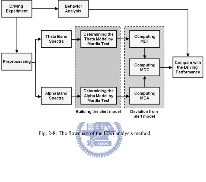
We developed the BCI system according to the steps of Fig. 2-1. The portable EEG acquisition module which we designed was used in input device of BCI. The EEG raw data continually transmitted to DSP module, hence, the following three steps: signal processing, features extraction, and classifier, were processed in DSP module. The algorithm we chose was according to unsupervised approach (N. R. Pal, 2008 [59]). The user interface can output real-time EEG signal and the results of drowsy detection on the screen of DSP module. If the results were judged to drowsiness by algorithm, DSP module will call the buzzer to output a warning voice to wake user up as a BCI application.

Fig. 2-1: A typical BCI system architecture

In off-line analysis, we wanted to verify the relationship between user’s driving trajectories and corresponding EEG signal. Before analyzing, we assumed that driving

(22)

module to observe and record driving information and actual EEG raw data at one time. We recorded 15 subjects’ EEG raw data and every one experimented 30 minutes. Our analysis included two parts: one was to analyze the driving trajectories, and another was to analyze the corresponding EEG signals. The first step of driving trajectories processing is to analyze the driving performance. On the other hand, we also analyze EEG signals. First, we use FFT to get the theta and alpha band information, and then using both two information built up an alert module, counting covariance matrix and mean vector of theta and alpha spectra. Furthermore, compute MDT, MDA, and MDC continually by using unsupervised method. After finishing both data analysis, we use binary classification test, sensitivity and specificity, to verify the drowsiness hit rate. Every experimental trial is separated and sorted, hence, the corresponding MD* (MDT, MDA, and MDC) will also be sorted. Defining the threshold of both information which been processed to decide the drowsiness or alertness, and to analyze the drowsy accuracy.

2.1 EEG Signal Acquisition

Electroencephalography (EEG) is the recording of electrical activity along the scalp produced by the firing of neurons within the brain. In clinical contexts, EEG refers to the recording of the brain's spontaneous electrical activity over a short period of time, usually 20–40 minutes, as recorded from multiple electrodes placed on the scalp [60]. When measuring from the scalps, recorded the EEG signal is about 10-100uV for a typical adult human. And a common system reference electrode is connected to the other input of each different amplifier. These amplifiers amplify the voltage between the active electrode and the reference (typically 1,000–100,000 times,

(23)

or 60–100 dB of voltage gain). The EEG is typically described in terms of rhythmic activity and transients. The rhythmic activity is divided into bands by frequency. The common band of EEG is shown as Table 2-1. Following the classification of EEG, Theta and Alpha band are related to drowsiness. Thus, when the subjects become drowsy, both bands will increase their power.

Table 2-1: Common band of EEG Type Frequency (Hz) Normally

Delta <4 Slow wave sleep for adults

Theta 4~7 Drowsiness, idling, or arousal in children and adults Alpha 8~12 Relaxed, reflecting, or closing the eyes

Beta 12~30 Alert or working

There are high correlation between drowsiness and EEG obtained from the location of OZ in the international 10–20 EEG system [61]. Therefore, in this study, we only monitored EEG in the location of OZ. Here, three EEG electrodes were used. One is input, one is reference, and the other is ground. According to a modified International 10–20 EEG system and refer to right ear lobe as depicted in Fig. 2-2. We use the following notations: F: Frontal lobe. T: Temporal lobe. C: Central lobe. P: Parietal lobe. O: Occipital lobe. "Z" refers to an electrode placed on the mid-line. The input data is placed in OZ, ground is fixed in the center of forehead, and reference is pasted behind the right ear.

(24)

Fig. 2-2: International 10-20 system

Raw EEG data were recorded with 12-bit quantization level at the sampling rate of 512 Hz. To simplify the computation, raw EEG data were down-sampled to sampling rate of 64 Hz. And a simple moving average filter was used to remove 60 Hz power line noise and other high-frequency noise.

2.2 Virtual Reality Driving Simulation Environment

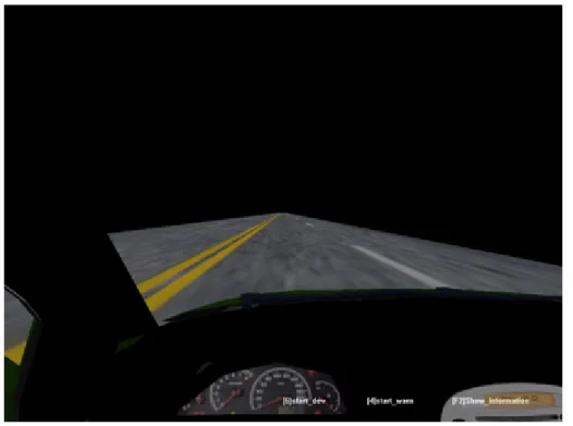
In this study, a lane-keeping driving experiment was utilized to investigate driving performance under different levels of drowsiness. Here, a virtual reality (VR)-based cruising environment was developed to simulate a car driving at 100 km/hr on a straight four-lane highway at night [54], [62]. During the driving experiments, all scenes move according to the displacement of the car and the subject’s maneuvering of the wheels which make the subject feel like driving the car on a real road. The VR environment is showing in Fig. 2-3.

(25)

Fig. 2-3: The overview of surrounded VR scene. The VR-based highway scenes are projected into surround screen with seven projectors.

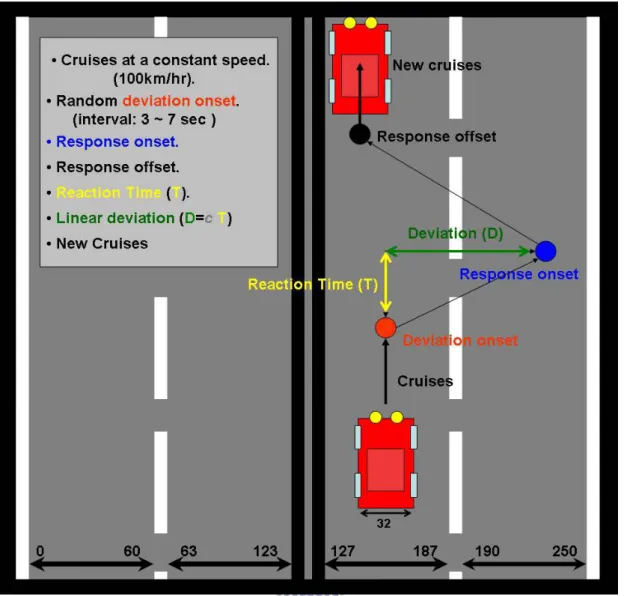
In all our experiments we have kept the driving speed fixed at 100 km/hr and system automatically and randomly drifts the car away from the center of the cruising lane to mimic the effects of a non ideal road surface. The driver is asked to maintain the car along the center of the cruising lane. All subjects involved in this study have good driving skill and hence when the subject is alert, his/her response time to the random drift is short and the deviation of the car from the center of the lane is small. But, when the subject is not alert / drowsy, both the response time and the car’s deviation are high. Note that, in all our experiments, the subject’s car is the only car cruising on the VR-based freeway. Although, both response time and the deviation from the central line are related to the subject’s driving performance, in this study, we use the car’s deviation from the central line as a measure of performance of the subjects. The driving task is showing in Fig. 2-4.

(26)

Fig. 2-4: The digitized highway scene. The width of highway is equally divided into 256 units and the width of the car is 32 units. An example of the deviation event. The car cruised with a fixed velocity of 100 km/hr on the VR-based highway scene and it was randomly drifted either to the left or to the right away from the cruising position with a constant velocity. The subjects were instructed to steer the vehicle back to the center of the cruising lane as quickly as possible [61].

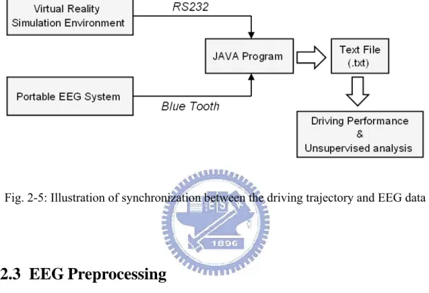
In order to synchronize the records of driving trajectory and raw EEG data, a JAVA program was designed to record both of them at the same sampling rate. The driving trajectory produced from the VR-based cruising environment environment program, and raw EEG data obtained by portable EEG acquisition module were transmitted to JAVA program via RS232 and Blue tooth respectively. After finishing

(27)

the experiment, both the driving trajectory and raw EEG data were saved in a text file. Then, we can investigate the correlation between driving performance and results of unsupervised approach. The illustration of synchronization between the driving trajectory and EEG data was shown in Fig. 2-5.

Fig. 2-5: Illustration of synchronization between the driving trajectory and EEG data

2.3 EEG Preprocessing

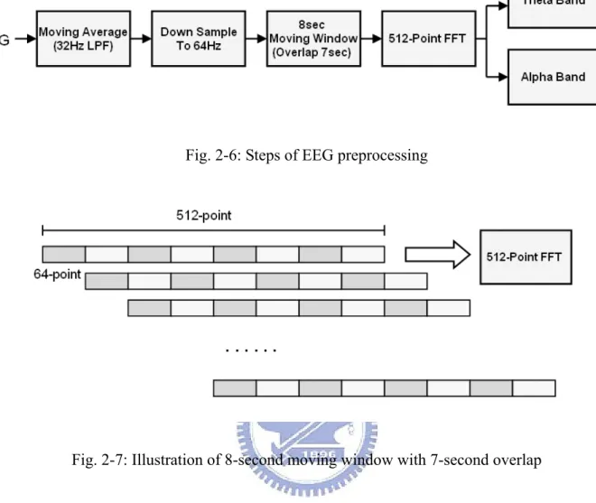
The EEG preprocessing steps were shown in Fig. 2-6. First, a simple moving average filter (low-pass filter with a cutoff frequency of 32 Hz) was used to remove 60 Hz power line noise and other high-frequency noise. In order to simplify the computation, raw EEG data were down-sampled to sampling rate of 64 Hz. Then, a 512-point moving window we designed to save the 8 seconds EEG information, as Fig. 2-7 shown. Finally, the power in the frequency band of alpha rhythm (8 ~ 11Hz) and theta rhythm (4 ~ 7Hz) was extracted.

(28)

Fig. 2-6: Steps of EEG preprocessing

Fig. 2-7: Illustration of 8-second moving window with 7-second overlap

2.4 Unsupervised Analysis

It is recognized that the changes in EEG spectra in the theta band (4~7Hz) and alpha band (8~11Hz) reflect changes in the cognitive and memory performance [63]. Other studies have reported that EEG power spectra at the theta band [64], [65] and/or alpha band [66], [67] are associated with drowsiness, and EEG log power and subject’s driving performance are largely linearly related.

As the above researches said, these findings have motivated us to derive the alert models of the driver using the alpha-band and theta-band EEG power spectrum computed using OZ channel output recorded in the first few minutes of driving. The

(29)

choice of the OZ channel is explained in the Experimental Results section. We emphasize that the few minutes of data used to find the alert model are not necessarily collected from the very beginning of driving session because different factors, such as walking of driver by a few meters to reach the garage, may influence the EEG signal generated at the very beginning. The specific window to be used for generation of the alert model is selected by Mardia test (explained later) [68]. We assume that if the subject/driver is in an alert state, then the EEG power spectra relating to theta band (as well as that relating to alpha band) would follow a multivariate normal distribution. The parameters of the multivariate normal distributions characterize the models. Using the alpha-band and theta-band EEG power, we identify two normal-distribution based models. Then, we assess the deviation of the current state of the subject from the alert model using Mahalanobis distance (MD). We assume that when the subject continues to remain alert, his/her EEG power should resemble the sample data used to generate the model and hence would match the alert model or template. If the subject becomes drowsy, then its power spectra in the alpha band (and also in theta band) will deviate from the respective model and hence MD will increase. With a view to reducing the effect of spurious noise, MDs are smoothed over a 90-sec moving windows, the window is moved by 1-sec steps [61]. We then study the relationship between smoothed Mahalanobis distance and subject’s driving performance by computing the correlation between the two. Fig. 2-8 shows the overall flow of the EEG data analysis. In this figure, note that, after the models are identified, the preprocessed alpha band and theta band power data directly go to the blocks for computation of MDA and MDT, respectively. MDT and MDA are measure of deviations of the subject’s present state from the respective models, this will be

(30)

analysis with the driver’s performance.

(31)

Chapter3

Hardware Frameworks

In this chapter, we focus on this portable system hardware. Following the design flowchart, we will introduce the design methods of hardware circuits and firmware structures steps by steps.

3.1 System Overview

In order to online measure and analyze EEG signals, the whole hardware framework of our BCI mainly contains two sub-systems: One is portable EEG acquisition module, and the other is DSP module. First, EEG signal was measured by our portable EEG acquisition module continually. After amplifying tiny EEG signals, noise except the frequency band of EEG would be removed by filters in our portable EEG acquisition module. And then, filtered EEG signals would be digitized by analog-to-digital converter, and be transited to the DSP module via Bluetooth. Here, Linux kernel µClinux was used as the operation system in DSP module to handle user’s applications. The major tasks of DSP module are to receive EEG signals via Bluetooth, and to execute the program of online drowsiness level detection, which monitor the variation of power of users’ alpha rhythm and theta rhythm. The program of online drowsiness level detection would collect EEG data under alertness for first 3 minutes to build EEG alert model, and then calculated drowsiness level by assessing the power variation of alpha and theta rhythm every 2 seconds. If the power variation exceeded the threshold of alert model, the DSP module would send warning tone of buzzer to wake up users. The whole hardware framework is shown as Fig. 3-1.

(32)

Fig. 3-1: Illustration of hardware framework of our BCI system

3.2 Portable EEG Acquisition Module

In order to be as small as possible and be easily wearable, a portable, distributive and wireless EEG headband system was designed to measure EEG signals. To reduce noise on PCB board produced by digital control circuit, the analog amplifier and digital control circuit were separated into two PCB boards. Following the previous researches [69], [70] worked, this general system was designed to minimize the circuit’s size, use a simple microcontroller to handle programs, implement filter more accurate, and etc. We also referenced some circuit designs [71]-[76]. Those circuit designs followed portable and wireless rules, separating the circuit into client and server model. In this session, we interested in the client circuit design. The portable EEG acquisition module system mainly contains five parts: (1) front-end filter circuit, (2) analog to digital converter, (3) digital controller, (4) power management circuit and (5) wireless transmission. The system block diagram is shown in Fig. 3-2.

(33)

Fig. 3-2: Block diagram of Portable EEG acquisition module

3.2.1 Front-End Filter Circuit

The front-end circuit consisted of preamplifier, and band-pass filter. The total gain of front-end circuit was set as about 5040 times with the frequency band of 0.1~100 Hz. In some references, other circuit designs liked to use unit gain filters and one variable gain amplifier. Moreover, they didn’t use a high-pass filter to cut-off the noise in low frequency band. To improve them, we designed a 3 stages high pass filter and 2 stages low pass filter to get the clear EEG information without noise. Hence, adding the gain into filter tried to minimize the total size.

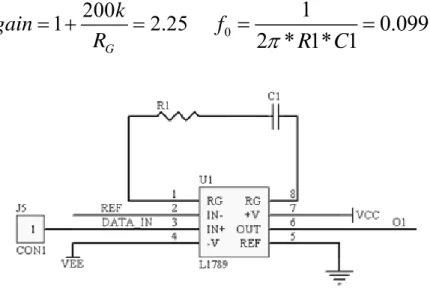
A. Preamplifier

Here, instrumental amplifier LT1789-1 was used as the first stage of analog amplifier. LT1789-1 owns an ultra low input current and a high common-mode rejection ratio (CMRR) about 90dB. A high CMRR is important in applications that the signal of interest is represented by a small voltage fluctuation superimposed on a (possibly large) voltage offset, or when relevant information is contained in the voltage difference between two signals. Here, instrumental amplifier LT1789-1 provided not only the function of gain, but also that of one stage high pass filter by

(34)

2.25 times. The instrumental amplifier circuit was shown in Fig. 3-3, and the simulation of preamplifier’s gain response was in Fig. 3-4.

200

1

2.25

G

k

gain

R

= +

=

₀

1

0.099 2 * 1* 1

f

R

C

π

=

Fig. 3-3: Circuits of preamplifier

9 8 10-4 10-3 10-2 10-1 100 101 102 103 0 1 2 3 4 5 6 7 X: 8.125 Y: 7.043 f (Hz) Ga in ( d B )

Fig. 3-4: Simulation of preamplifier’s gain response

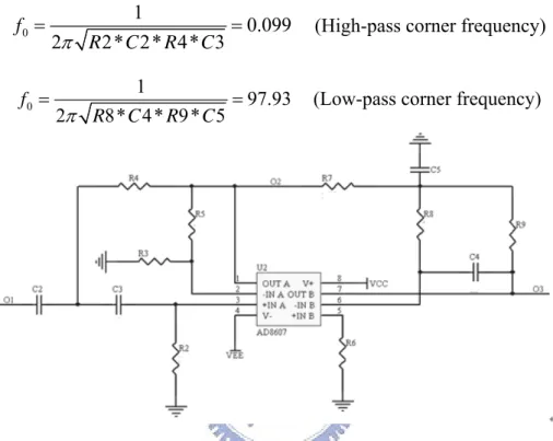
B. Band pass filter

In order to more precisely reserve relevant EEG signal, a band pass filter with frequency band of 0.1Hz ~ 100Hz and with gain of 1588.75 times was designed. The band-pass filter consisted of a 2nd-order high-pass filter and a 2nd-order low-pass

(35)

filter. Here, OP-AMP AD8607 was used to construct the band-pass filter. AD8607 also owns high CMRR (about 100dB), low input current, low distortion, and no phase reversal. The band-pass filter circuit was shown in Fig. 3-5, and the simulation of those gain response was in Fig. 3-6.

0 1 0.099 2 2* 2* 4* 3 f R C R C π

= = (High-pass corner frequency)

0 1 97.93 2 8* 4* 9* 5 f R C R C π

= = (Low-pass corner frequency)

Fig. 3-5: Circuits of band-pass filter

10-4 10-3 10-2 10-1 100 101 102 103 104 105 106 0 10 20 30 40 50 60 70 80 X: 2.64 Y: 66.58 f (Hz) Ga in ( d B)

(36)

The system specification of portable EEG acquisition module is listed below. The damping ratio of second order filter was set to 0.5, thus, the Bode diagram could be smoother in two sides of 3dB point as Table 3-1 descript. The final simulation of gain response was shown in Fig. 3-7.

Table 3-1: System specification of IA, HP, and LP filter for portable EEG acquisition module

Orders Type Gain Corner Freq. Damping

Instrumental amplifier Quasi HP 2.25 0.099

High-pass filter HP 43.7 0.099 0.5 Low-pass filter LP 51.25 97.93 0.707 100 10-4 10-3 10-2 10-1 100 101 102 103 104 105 106 0 10 20 30 40 50 60 70 80 90 X: 2.93 Y: 73.62 f (Hz) Gai n ( d B)

(37)

3.2.2 Analog to Digital Converter

The analog amplifier circuit and digital control circuit of our portable EEG acquisition module were placed individually in two PCB boards. There are some leading wires to connect both. A 12-bits analog-to-digital converter (ADC) AD7466 was used to convert continuous EEG signal of analog amplifier circuit to digitized EEG signal. Here, the micro-controller (MSP430F1611) was used to control ADC AD7466. The handshake mode between MSP430F1611 and AD7466 was shown in Fig. 3-8. The command signals and serial digitized EEG signal were transmitted via the serial peripheral interface (SPI) of MSP430F1611. The micro-controller MSP430F1611 outputs SCLK and CS signals in specific sampling rate 512Hz, and then digitized EEG signal would deliver into MSP430F1611. Each converting interval needed 16 cycles to complete transmission of digitized data, here, the data in first 4 cycles were zero, and the others were real 12-bit digitized data based on MSB.

Fig. 3-8: Handshake mode between AD7466 and MSP430F1611

Moreover, according to equation (3-1), the conversion time is about 4.7 μs, and 8-bit digitized data were transmitted every transmission cycle. And the maximum frequency of input signal of ADC was 100Hz. After calculating in equation (3-2) and (3-3), the result conforms to the equation (3-1). Thus, this system needn’t a sample

(38)

1 in a dV t LS dt ⎛ _× ⎞_≤ ⎜ ⎟ ⎝ ⎠ B (3-1) 8

3 0.0117

2 V

LSB

=

(3-2) ^ 2 3 2 100 4.7 0.00886 in a a dV t V f t dt

π

μ

⎛ _× ⎞_{= ×} _{× = ×} _× _× ₌ ⎜ ⎟ ⎝ ⎠ (3-3)

3.2.3 Digital Controller

The TI micro-controller MSP430F1611 was utilized to control other parts of circuits in portable EEG acquisition module. It owns many advantages for medical application, includes ultra-low power consumption, 16-bit RISC architecture, 125 ns instruction cycle time, five power saving modes, and diversification of peripheral communication interface. The functional block diagram of MSP430F1611 was shown in Fig. 3-9.

Fig. 3-9: Functional block diagram of MSP430F1611

(39)

peripheral interface with sampling rate 512Hz, and then digitized EEG data were stored into memory of MSP430F1611. Next, a moving average filter was used to remove 60-Hz power line interference before wireless transmission. The operating flow chart in MSP430F1611 was shown in Fig. 3-10.

Fig. 3-10: Operating flow chart in MSP430F1611

A. Timer Interrupt

The interrupt function of MSP430F1611 is based on inner timer/counter register, called Timer_A, to count a specific time value. The counter value TACCR0 had to be set first, as shown in Fig. 3-11. When the timer counted to the TACCR0 value, the TACCR0 CCIFG interrupt flag would be set. And when the timer counted from TACCR0 to zero, the TAIFG interrupt flag would be set. In our portable EEG acquisition module, 4MHz crystal oscillator was used as system clock of MSP430F1611, and the sub-system master clock was set to 2MHz. Therefore, the operating cycle of program in MSP430F1611 would follow sub-system master clock. Thus, if the sampling rate of our EEG acquisition module is set to 512 Hz, TACCR0 has to be set to 3906.

2M

(40)

Fig. 3-11: Timer_A up mode for interrupt function of MSP430F1611

B. SPI Mode

In synchronous mode, the USART of MSP430F1611 connects to external systems via three or four pins: SIMO, SOMI, UCLK, and STE, as shown in Table 3-2.

Table 3-2: Definition and function for pins of SPI mode SPI Mode Operation

SIMO Slave in, master out SOMI Slave out, master in UCLK USART SPI clock

STE Slave transmit enable. Not used in 3-pin mode.

The master configuration of USART was shown in Fig. 3-12. The data transmission function of USART was initiated when transmitted data were moved to the transmit data buffer UxTXBUF. If the TX shift register was empty, then data in UxTXBUF would be moved into the TX shift register. When transmitted data were received, the received data were moved from the RX shift register to the received data buffer UxRXBUF and the receive interrupt flag URXIFGx would be set, that indicates the RX/TX operation was completed.

(41)

cascade-connect with four front-end circuits via SPI, as shown in Fig. 3-13. Therefore, the handshake connection between Master module and Slave module needs 3-pin to transmit data: CS, SOMI, and UCLK. And there are four CS signal lines, one SOMI, and one UCLK signal line inside the leading wire.

Fig. 3-12: USART Master and external Slave

Fig. 3-13: Illustration for connection between four front-end circuits and digital control circuit

C. Moving Average

Moving average, also called rolling average or running average, is usually used to analyze a set of data points by creating a series of averages of different subsets of the full data set. Moving average can be applied to any data set, however, it is most

(42)

the setting of moving average parameters depends on the requirement of application. Mathematically, moving average is a type of convolution and is similar to a low-pass filter used in signal processing. The moving average filter is optimal for a common task: reducing random noise while retaining a sharp step response. This makes it as the premier filter for time domain encoded signals.

Given a sequence

{ }

N₁, the output of an n-moving average is a new sequence i _i a ₌

{ }

1 1 N n i i

s ₌− + defined as the average of subsequences of n terms. The formula of moving

averaging was shown as followings.

1 1 1i n i j s n + − = =

∑

aj (3-4)

Therefore, the sequences s_n of n-moving averages when n=2,3 can be expressed

as

(

)

2 1 2 2 3 1 1 , ,..., 2 n n s = a +a a +a a₋ +a

(

)

3 1 2 3 2 3 4 2 1 1 , ,..., 3 n n s = a +a +a a + +a a a ₋ +a ₋ +an (3-5)

Fig. 3-14 shows the results of noise cancellation by using moving average. Here, a function generator was used to generate sin wave, and our portable EEG acquisition module was used to record this signal. If our portable EEG acquisition module was close to some electric instruments, the signal recorded from EEG acquisition module would easily be influenced by noise of 60 Hz power line. In the above figure of Fig. 3-14, it showed that the original sib wave had been contaminated by 60Hz power-line noise. After filtering by using moving average with 9-point moving window, we found moving average could effectively remove power-line noise, as shown in the below figure of Fig. 3-14.

(43)

512 _ _ SampleRate₆₀ ₆₀ 8.53 Num of window= = = (3-6) 3000 3020 3040 3060 3080 3100 3120 3140 3160 3180 3200 50 100 150 200

Befor Moving average

Am p Sample 3000 3020 3040 3060 3080 3100 3120 3140 3160 3180 3200 50 100 150 200

After Moving average

Am

p

Sample

Fig. 3-14: Result of noise cancellation by using moving average

D. UART Interface

In asynchronous mode, USART connected MSP430 to external systems via two external pins, URXD and UTXD. In UART mode, USART transmitted and received characters at a bit rate asynchronously to another device. Timing for each character was based on the selected baud rate of USART. Here, the transmitter and receiver used the same baud rate. For initializing UART, RX and TX had to be enable first, and then decided the baud rate of UART and disable SWRST. The required division factor N for determining baud rate was listed as followings:

BRCLK N

baud rate

= (3-7) Here, BRCLK was 4 MHz, and baud rate was 115200 bit/s. After initializing

(44)

3.2.4 Power Management

Power Management circuit in our portable EEG acquisition module includes two parts: one is power supply circuit, and the other is charging circuit.

A. Power Supply Circuit

In our portable EEG acquisition module, the operating voltage VCC was at 3V, and the virtual ground of analog circuit was at 1.5V. In order to provide stable 1.5V and 3V voltage, a regulator LP3985 was used to regulate battery voltage to 3V. Here, LP3985 is a micro-power, 150mA low noise, and ultra low dropout CMOS voltage regulator. The maximum output current can support 550mA. Furthermore, the turn-on time can reach 200μs. And a voltage divider circuit was used to divide 3V voltage into 1.5V, and a unity amplifier constructed from AD8628 was used to provide a voltage buffer. The total power supply circuit was shown in Fig. 3-15.

Fig. 3-15: Power supply circuit in portable EEG acquisition module

(45)

B. Charging Circuit

The charging circuit BQ24010DRC had integrated power FET and current sensor for 1-A charging applications. The maximum charging current can arrive to 1A. The battery’s power would be detected automatically by charging circuit and switched to charging mode when battery’s power was not enough. BQ24010DRC also protected battery to avoid over charging or over driving [77]. The charging circuit was shown in Fig. 3-16.

Fig. 3-16: Charging circuit in our portable EEG acquisition module

3.2.5 Wireless Transmission

Bluetooth is a wireless protocol utilizing short-range communication technology to facilitate data transmission over short distances from fixed and/or mobile devices. The intent behind the development of Bluetooth was the creation of a single digital wireless protocol, capable of connecting multiple devices and overcoming issues

(46)

BM0203 was used. BM0203 is an integrated Bluetooth module to ease the design gap and uses CSR BuleCore4-External as the major Bluetooth chip. CSR BlueCore4-External is a single chip radio and baseband IC for Bluetooth 2.4GHz systems including enhanced data rates (EDR) to 3Mbps. It interfaces to 8Mbit of external Flash memory. When used with the CSR Bluetooth software stack, it provides a fully compliant Bluetooth system to v2.0 of the specification for data and voice communications. All hardware and device firmware of BM0203 is fully compliant with the Bluetooth v2.0 + EDR specification. Bluetooth operates at high frequency band to transmit wireless data, so it can be perfect worked by using a PCB antenna, as shown in Fig. 3-17.

Fig. 3-17: PCB Blue Tooth antenna [77]

3.3 DSP Module

The design goal of DSP module is to build a back-end analysis platform. This platform not only has greatly powerful calculating ability, but also supports various peripheral interfaces. After measuring and pre-processing EEG signal by our portable EEG acquisition module, EEG signal would be transmitted to this DSP module via Bluetooth module. DSP module would then process and analyze EEG signal, and display results of EEG analysis on TFT LCD. Furthermore, it also can use other

(47)

peripheral interfaces to implement other applications [77].

3.3.1 DSP Framework

A powerful digital signal processor Analog Device BF533-STAMP was used in this DSP module, and its CPU speed can be up to 600MHz. It owns two 16-bit MAC, Multiply-And-Accumulate, to execute 1200 lines addition and multiplication functions. By the way, DSP contains many independent DMA, Direct Memory Access, to effectively reduce the processing time of core. The system block diagram was shown in Fig. 3-18. Here, Bluetooth module and UART both worked in the same UART interface.

TFT-LCD, worked by using Memory Mapping, shared the same Memory Bus with SDRAM. In order to reduce the size of platform, we decided to replace traditional parallel NOR Flash with SPI Flash, and it also shared with SD/MMC Socket. Furthermore, the DSP module also owned power management and charging circuits. SD/MMC Socket provided the interface scalability, such as SD/MMC Card, Sensor, ADC, Wireless Card, etc. In our application for drowsiness detection and warning, an expanded SD card circuit which can plug in SD card socket of DSP module was designed to produce buzzer. This circuit will be introduced in next session.

(48)

Fig. 3-18: The block diagram of DSP system [77]

3.3.2 The Expanded SD Card Circuit

The expanded SD card circuit was designed to expand the function of DSP module. DSP module and expanded SD card circuit communicated with each other via SPI interface. Here, DSP module was set as Master configuration, and expanded SD card circuit was set as Slave configuration, as shown in Fig. 3-19.

Fig. 3-19: Handshake mode between DSP module and expanded SD card circuit In this expanded SD card circuit, another microcontroller MSP430F2013 was

(49)

used as the core of this circuit. This controller only has 14 pins and its size is 5.1 mm x 6.2 mm. MSP430F2013 can provide many benefits, such as inner 32768 Hz oscillator, two pair I/O ports, USI (Universal Serial Interface) interface, Timer interrupt, watch dog timer, 16-bit Sigma-Delta Analog to Digital converter, etc. The expanded SD card circuit included a microcontroller, an ICE download pin, SD/MMC interface connection, a buzzer, and a LED. The function block diagram was shown in Fig. 3-20. The schematic circuit of expanded SD card circuit was shown in Fig. 3-21.

(50)

Fig. 3-21: Schematic circuit of expanded SD card circuit

The operating flow chart of expanded SD card circuit was shown in Fig. 3-22. Here, MSP430F2013 in expanded SD card circuit always waited to receive commands from DSP module. When command data was arrived, expanded SD card circuit would start USI interrupt. Second, the command data for expanded SD card circuit was defined as two different warning modes. In mode one, low frequency warning tone would be generated by an interval PWM, and in mode two, high frequency warning tone would be generated by a high potential signal.

(51)

Fig. 3-22: Operating flow chart of expanded SD card circuit

3.4 Hardware System Implementation

A. Portable EEG acquisition module

Fig. 3-23(a ~ c) are the front-end analog circuit and digital control circuit in our portable EEG acquisition module, and the whole EEG acquisition module respectively, and the size of each circuit compared with a coin of one NTD was shown in Fig. 3-23. There are three leads in our portable EEG acquisition module, includes EEG input, reference, and virtual ground of the front-end analog circuit. The electrodes connected

(52)

and behind right ear respectively. The specification of portable EEG acquisition module was listed in Table 3-3.

(a)

(b)

(c)

Fig. 3-23: (a) The front-end analog circuit, (b) the digital control circuit, and (c) the whole portable EEG acquisition module with single channel.

(53)

Table 3-3: The spec of portable EEG acquisition module Type Portable EEG Acquisition Module

Channel Number 1~8

System Output Voltage Range 0~3V

Gain 5000 Bandwidth 0.1~100Hz

ADC Resolution 12bits

Output Current 29.5mA

Battery Lithium 3.7V 450mAh 15~33hr Full Scale Input Range 577μV

Sampling 512Hz Input Impedance greater than 10MΩ

Common Mode Rejection Ratio 77dB Power Supply Rejection Ratio 88dB

Size 18mm x 20mm and 25mm x 40mm

B. DSP Module and SD Card Circuit

The expanded SD card circuit was shown in Fig. 3-24(a). It looked like a SD/MMC card, which can easily be plugged into the SD/MMC socket in DSP module. The size of expanded SD card circuit is 24mm x 32mm. Fig. 3-24(b) is the illustration for application of expanded SD card circuit.

(54)

(a)

(b)

Fig. 3-24: (a) The expanded SD card circuit and (b) illustration for application of expanded SD card circuit

(55)

Chapter4 Unsupervised Approach

Based on the unsupervised analysis flowchart in Fig. 2-8, we will further discuss the details of every analysis diagrams in the following sessions. In order to find out the real driving behavior information, first we calculate the driver’s driving performance by using the record in simulation experiment. Moreover, we use the unsupervised analysis method to analyze the corresponding EEG information, including the preprocessing, alert model construction, and computation of the deviation using Mahalanobis distance method.

4.1 Driving Performance

The VR-based four-lane straight highway scene was applied in the experiment. In this scene, the four lanes from left to right are separated by a median stripe and the distance from the left side to the right side of the road was equally divided into 256 points indicating the position of the vehicle as the digital output signal of the VR scene at each time instant. The width of each lane and the car is 60 units and 32 units, respectively. Fig. 2-4 shows an example of the driving performance represented by the vehicle deviation trajectories. We have defined an indirect index of the subject’s alertness level (driving performance) as the deviation between the center of the vehicle and the center of the cruising lane. VR driving simulation environment will randomly start a deviation event to move the car to right or left side in the car driving experiments. Subjects needs to sense those sudden movements and trying to make a reversely turn to back to the third lane. At one time, the VR environment also outputs

(56)

deviation event.

Fig. 4-1: The example of deviation event and car trajectories

In Fig. 4-2, the driving trajectories that we recorded followed below steps to show the driving performance. For restoring trajectories data, event trigger removal is the first process that we do. After deviation response offset, the positions of every experiment trial aren’t consistent, so that we need to remove the baseline every trial. The results of the second step will leave right or left turn trajectories. And then absolute trials to collocate total right / left turn data. Typically the drowsiness level fluctuates with cycle lengths longer than 4 minutes [64], [65], and hence we smooth the indirect alertness level index using a causal 90-sec moving window advancing. This helps us to eliminate variance with cycle lengths shorter than 1-2 minutes. We emphasize that this index is used only to validate our approach, and it is not as an input to develop the model for the alert state of the subject.

Fig. 4-2: The processing steps of driving performance

(57)

Fig. 4-3. Fig. 4-3(a) shows the original driving data which including event triggers, and Fig. 4-3(b ~ d) shows the results of 4 steps respectively. The final driving performance is in Fig. 4-3(e). Thus, we use this result to compare with MD*(MDT, MDA, and MTC) and implement in correlation analysis with the driver’s performance.

Fig. 4-3: Example of driving performance analysis. (a ~ d) are the fragment of information which marked by two lines. (a) is the original driving trajectories data which including deviation event triggers. (b) is the result which has passed through event trigger removal. (c) is the absolute result. (d) is the result which has smoothed by 90-sec moving average. (e) shows the total driving performance data.

(58)

4.2 Smoothing of the Power Spectra

Before extracting the power spectra of alpha and theta rhythms, raw EEG data would be preprocessed to remove power line noise and increase the resolution in the low frequency spectra. In this smoothing method, we used a moving average, as a low-pass filter to cut-off at 32 Hz in and filter noise over 32 Hz. A moving average filter was used to minimize the presence of artifacts in the EEG records of all sub-windows. Next, we down sample 8 times to 64Hz, so that every sub-window only left 64 points in one second. Those two preprocessing methods can decrease the unnecessary noise and increase the low frequency band information in theta and alpha band spectra. Go on, building up an 8 second moving window to save sub-windows, and displace a sub-window in every 1 second. The first FFT result will be produced at 8th seconds; moreover other FFT results will be in every following 1 second. The smoothing method of moving window can reserve the low frequency information of EEG power spectra longer to further analysis. Thus, for each session EEG log power time series at alpha band as well as at theta band with 1 sec time intervals were generated. Fig. 4-4 showed the processes of spectra analysis as precedence.

(59)

Fig. 4-4: Processes of spectra analysis as precedence

4.3 Construction of the Alertness Model

To investigate the relationship between the measured EEG signals and subject’s cognitive state, and to quantify the level of the subject’s alertness in our previous studies [78]-[80], first, we need to quantify the volunteer’s drowsiness level in this experiment. When subjects fall drowsy, they often exhibit relative inattention to environments, eye closure, less mobility, failure to motor control and making decision. Hence, the vehicle deviations were defined as the subject’s drowsiness index.

In our approach for every subject in every driving session a new model will be constructed. Consequently the variability between subjects as well as the inter-session variability is no more important; these are taken into account automatically. To develop the alert model we make a few mild but realistic assumptions as follows: (1) The subject is usually very alert immediately after he/she starts the driving

(60)

(2) Subject’s cognitive state can be characterized by the power spectrum of his/her EEG.

(3) When the person is in the alert state, it can be modeled reasonably well using a multivariate distribution of the power spectrum.

(4) The alert model expresses well the EEG spectra when the subject remains alert or return to alert state from drowsiness.

One can argue that the subject may already be in a drowsy state when he/she begins driving. If that is really true, then that can be detected by checking the consistency between two alert models derived using data in two successive time intervals. In other words, we can check whether the two alert-models identifies in two successive time intervals are statistically same or not. If the subject was already in a drowsy state, then he/she will either move to a deep drowsy/sleepy state or will transit to an alert state. In both cases, the two models will not be statistically consistent.

Here we use a multivariate distribution to model the distribution of power spectrum in the alert state. In particular, at every 1 second, we calculate the power spectrum vector in p dimension. In our experiment theta band is located in 32~63 (4~7Hz), and alpha band is in 64~96 (8~12Hz). In this way, a set of n=60 data vectors {x1,…,x60} is generated in every minute. We use 3 minutes of spectral data to derive

the alert model. The alert model is represented and characterized by a multivariate normal distribution N(_μ,_Σ2) , where _{μ is the mean vector and is the} variance-covariance matrix.

Σ

We use the maximum likelihood estimates for μ and_{Σ . After finding the alert}2

model we check whether the EEG spectrum in the alpha band (also in theta band) indeed follows a multivariate normal using Mardia’s test [81], [82]. If the model passes the Mardia’s test, we accept that model as the alert model. Otherwise, we move

(61)

the data window by one minute and again use the next 3 minutes of data to derive and validate the model using Mardia’s test. Once a model is built, a significant deviation from the model can be taken as a departure from alertness. Note that, we are saying “departure from alertness” which is not necessarily drowsiness. For example, the subject could be excited over a continued conversation over a mobile phone. In this case, although the person is not drowsy, he/she is not alert as far as the driving task is concerned and hence needs to be cautioned. Thus our approach is more useful than typical drowsiness detection systems. A consistent and significant deviation for some time can be taken as an indicator of drowsiness.

For the sake of completeness, we briefly explain the Mardia’s test of multi-variate normality. Given a random sample, X={x1,…,xn} in Rp, Mardia [81],

[82] defined the p-variate skewness and kurtosis as:

3 1 1 1 2 , 1 {( ) ( )} 1 b = x −x ′ − x −x = =

∑∑

j n i n j i p S n (4-1) 2 1 1 , 2 ( ) ( )} 1 x x x x − ′ − = − =

∑

i n i i p S n b (4-2)

In (1) and (2)

x

and S represent the sample mean vector and covariance matrix, respectively. In this case of university data, b1,p and b2,p reduces to the usual university

measures skewness and kurtosis, respectively. If the sample is obtained from a multivariate normal distribution, then the limiting distribution of b1,p is a Chi-square

with p p( +1)(p+2) /6 degrees of freedom, while that of ) 2 ( 8 / )) 2 ( (

n b₂_,_p− p p+ p p+ is N(0,1). Hence we can use these statistics to test multi-variety normality. In all our experiments, we have used the routines available

(62)

4.4 Computation of the Deviation from the Subject

After the alert model is found, we use it to assess the subject’s cognitive state. This was done by finding how the subject’s present state, as represented by the EEG power spectra, and was different from the state represented by the alert model. The deviation of the present state from the model is computed using Mahalanobis distance [84] that can account for the covariance between variables while computing the distance. Let the alert model computed using the alpha band be represented by

( , )

x

S

_A and that by the theta band be represented by

( , )

x

S

_T. Let x be a vector representing the power spectra in the alpha band (or in the theta band) of the EEG of the subject at some time instant, then the deviation of the present state from the model is:

T -1

MD*( ) ( - ) S ( - )x = x x x x (4-3)

In (3) if we use the alpha band model, then * is A, and for the theta band model and data, * will be T. Thus the deviation from the alpha band model will be denoted by MDA and that for the theta band model will be denoted by MDT. Similar to the pre-processing of the indirect alertness level index (driving performance), the MDA/MDT is also smoothed by the moving average method using a window with a window of 90 seconds. The moving average window is shifted by just one value (i.e., 2 sec). For a better visual display, we have scaled the MD* values by subtracting the average MD* computed over the training data used for finding the alert model.

We shall see later that the deviation from either the alpha band model (i.e., MDA) or the theta band model (i.e., MDT) can be used to detect departure from the alart

即時無線瞌睡偵測腦機介面系統

國 立 交 通 大 學

電機與控制工程學系

碩 士 論 文

即時無線瞌睡偵測腦機介面系統

Real-time Wireless Brain Computer Interface for

Drowsiness Detection

研 究 生：張哲睿

指導教授：林進燈 博士

中華民國 九十八 年 七 月

即時無線瞌睡偵測腦機介面系統

Real-time Wireless Brain Computer Interface for Drowsiness

Detection

研 究 生：張哲睿 Student：Che-Jui Chang

指導教授：林進燈 博士

Advisor：Dr. Chin-Teng Lin

國立交通大學

電機與控制工程學系

碩士論文

A Thesis

Submitted to Department of Electrical and Control Engineering

College of Electrical Engineering

National Chiao Tung University

in Partial Fulfillment of the Requirements

for the Degree of Master

in

Electrical and Control Engineering

July 2009

Hsinchu, Taiwan, Republic of China

即時無線瞌睡偵測腦機介面系統

學生：張哲睿

指導教授：林進燈 博士

國立交通大學電機與控制工程研究所

摘要

Real-time Wireless Brain Computer Interface for

Drowsiness Detection

Student: Che-Jui Chang

Advisor: Dr. Chin-Teng Lin

Department of Electrical and Control Engineering

National Chiao Tung University

Abstract

誌謝

Contents

List of Tables

List of Figures

Chapter1 Introduction

1.1 Brain Computer Interface

1.2 Previous Research

1.3 Motivation

1.4 Organization of Thesis

Chapter2 Material and Method

2.1 EEG Signal Acquisition

2.2 Virtual Reality Driving Simulation Environment

2.3 EEG Preprocessing

2.4 Unsupervised Analysis

Chapter3

Hardware Frameworks

3.1

System Overview

3.2 Portable EEG Acquisition Module

3.2.1 Front-End Filter Circuit

200

1

2.25

k

gain

R

= +

=

1

0.099

2 * 1* 1

f

R

C

π

=

=

3.2.2 Analog to Digital Converter

3

國立交通大學

碩士論文

研究生：張哲睿

指導教授：林進燈博士

中華民國九十八年七月

研究生：張哲睿 Student：Che-Jui Chang

指導教授：林進燈博士

指導教授：林進燈博士