Multigrid Methods for Incompressible Heat
Flow Problems with an Unknown Interface
C. W. Lan∗,1and M. C. Liang†
∗Chemical Engineering Department, National Taiwan University, Taipei, Taiwan 106, Republic of China; and
†Chemical Engineering Department, National Central University, Chung-Li, Taiwan 320, Republic of China E-mail: [email protected]
Received April 17, 1998; revised January 29, 1999
Finite-volume/multigrid methods are presented for solving incompressible heat flow problems with an unknown melt/solid interface, mainly in solidification ap-plications, using primitive variables on collocated grids. The methods are imple-mented based on a multiblock and multilevel approach, allowing the treatment of a complicated geometry. The inner iterations are based on the SIMPLE scheme, in which the momentum interpolation is used to prevent velocity/pressure decoupling. The outer iterations are set up for interface update through the isotherm migration method. V-cycle and full multigrid (FMG) methods are tested for both two- and three-dimensional problems and are compared with a global Newton’s method and a single-grid method. The effects of Prandtl and Rayleigh numbers on the performance of the schemes are also illustrated. Among these approaches, FMG has proven to be superior on performance and efficient for large problems. Sample calculations are also conducted for horizontal Bridgman crystal growth, and the performance is compared with that of traditional single-grid methods. ° 1999 Academic Pressc
Key Words: multigrid; finite-volume method; solidification; interface.
1. INTRODUCTION
Solidification processes, such as casting and crystal growth, involve incompressible heat flow and an unknown shape of the solidification (growth) front. In such systems, in addition to complicated geometry, simulation could become quite challenging due to the strong cou-pling of incompressible heat flow and the unknown melt/solid interface shape. Especially, for high Prandtl number materials, the interface is affected significantly by convection. Sev-eral numerical approaches [e.g., Refs. 1–8] for solving such problems have been proposed. They can be categorized, from the formulation point of view, by streamfunction/vorticity (ψ/ω) [2, 3, 6, 7] and primitive (UVP) variables [1, 4, 5, 8], and from the solution point
1To whom correspondence should be addressed.
55
0021-9991/99 $30.00 Copyright c° 1999 by Academic Press All rights of reproduction in any form reserved.
of view, by decoupled [2–6] and global (coupled) [1, 7, 8] iteration approaches. The global approaches [1, 7, 8] have shown great robustness, and with the iterative matrix solver they are much more efficient than direct solvers for larger problems. However, as compared with traditional decoupled point or line iteration schemes, for large problems, especially for three-dimensional (3D) problems, the iterative matrix solvers still require a tremendous amount of computer memory and often need the use of supercomputers. This has discour-aged the performance of their 3D calculations in an engineering workstation. Theψ/ω approach, which requires more equations for 3D problems, is less efficient than the UVP approach. Accordingly, the decoupled UVP method seems to be a better choice for large 3D applications.
The use of a decoupled method [e.g., 2–6], especially the point iteration approach, could greatly reduce the memory required. However, most iterative schemes, e.g., the Gauss– Siedel method, are good smoothers only for short wavelength errors [9]. For long wave-length errors, the convergence rate is slow. For large problems, the convergence rate thus degrades very quickly as the iteration proceeds, especially as the grid is refined. The con-vergence rate becomes slower as the problem size increases. Accordingly, multigrid (MG) methods that use different meshes to smooth errors with a wider spectrum of wavelengths have been used widely to overcome the difficulty of slow convergence [9, 10]. Very often, if the implementation is right, the convergence is not affected by the problem size, and its operation counts are linearly proportional to the problem size as well. Accordingly, MG methods have been regarded as one of the most effective methods in the computational fluid dynamics (CFD) community [11, 12]. Many studies [e.g., 13, 14] have reported the suc-cessful implementation of MG on incompressible flow applications, and its performance is very impressive. However, applications to free-boundary or free-interface problems are very limited. The work by Farmer et al. [15] seems to be the only application of MG to the free-surface problem. No applications of MG methods to solidification problems, i.e., with a melt/solid interface, have been reported.
In the present report, approaches implementing the isotherm migration method (IMM) upon a MG incompressible flow solver are presented for solidification problems. The incom-pressible flow solver design is based on a multiblock and multilevel concept for the treat-ment of complicated geometry. In each block/level, a collocated-grid finite-volume method (FVM) is used, in which the SIMPLE scheme [16] is used as a smoother. The strategies for interface update based on both V-cycle and full MG (FMG) methods are compared for 2D and 3D problems. A global Newton’s method used in our previous report [8] is also tested for comparison purposes. In the next section, the physical model used is described. The FVM/MG implementation based on the multiblock and multilevel concept is discussed in Sections 3 and 4. Section 5 is devoted to results and discussion, followed by conclusions in Section 6.
2. FORMULATION FOR PHYSICAL PROBLEMS
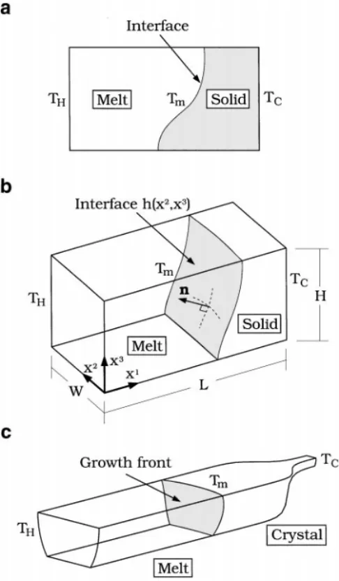
The 2D and 3D steady-state two-phase heat flow problems studied in this report are shown in Figs. 1a and 1b, respectively. The material is partially solidified in a cavity; the interface is coupled with heat transfer and fluid flow. The upper surface can be either a free surface or a solid wall. A simple extension of the two-phase problem is shown in Fig. 1c for horizontal Bridgman (HB) crystal growth, which is one of the major processes
FIG. 1. Schematics of the two- and three-dimensional two-phase heat flow problems: (a) two dimensional (2D), (b) three dimensional (3D), and (c) horizontal Bridgman crystal growth.
for growing GaAs single crystals [17]. In the HB process, the upper surface is usually open to the gas environment and is thus a free surface. To focus on the numerical study, we have purposely chosen Fig. 1b for the formulation of governing equations. Other applications can be extended from here easily [e.g., Refs. 18, 19].
As illustrated in Fig. 1b, the temperature on the two ends is fixed; the left temperature TH
is higher than the melting point (Tm) of the material inside, while the right temperature TC
is lower. The other sides of the system are assumed adiabatic. Again, the case with heat loss or fixed temperature can also be treated easily if needed. The melt/solid interface position
h(x2, x3) is unknown a priori, and needs to be solved simultaneously with other field
variables. In the applications of crystal growth, which are our major interests, the movement of the system (in the order of mm/h) is much slower than the melt velocity. Therefore, the contribution due to the movement of the system is considered only at the interface to take the heat of fusion into account. The melt is assumed incompressible and the flow laminar. The dimensionless variables are defined by scaling the length with the height H , velocity withαm/H, and pressure with ρmα2m/H2, whereαmis the thermal diffusivity andρm
With the Boussinesq approximation [20], the conservation equations in dimensionless form for 3D steady incompressible laminar flow of a Newtonian fluid in the melt, and heat conduction in the solid, can be described as follows:
Melt ∂u1 ∂x1 + ∂u2 ∂x2 + ∂u3 ∂x3 = 0, (1) ∂ ∂x1 µ u1u1− Pr ∂u1 ∂x1 ¶ +∂x∂2 µ u2u1− Pr ∂u1 ∂x2 ¶ +∂x∂3 µ u3u1− Pr ∂u1 ∂x3 ¶ +∂x∂ P1 = 0, (2) ∂ ∂x1 µ u1u2− Pr∂u 2 ∂x1 ¶ + ∂ ∂x2 µ u2u2− Pr∂u 2 ∂x2 ¶ + ∂ ∂x3 µ u3u2− Pr∂u 2 ∂x3 ¶ + ∂ P ∂x2 = 0, (3) ∂ ∂x1 µ u1u3− Pr ∂u3 ∂x1 ¶ +∂x∂2 µ u2u3− Pr ∂u3 ∂x2 ¶ + ∂ ∂x3 µ u3u3− Pr ∂u3 ∂x3 ¶ + ∂ P ∂x3 − Ra Pr θ = 0, (4) ∂ ∂x1 µ u1θ − ∂θ ∂x1 ¶ + ∂ ∂x2 µ u2θ − ∂θ ∂x2 ¶ + ∂ ∂x3 µ u3θ − ∂θ ∂x3 ¶ = 0. (5) Solid κs · ∂ ∂x1 µ∂θ ∂x1 ¶ +∂x∂2 µ∂θ ∂x2 ¶ +∂x∂3 µ∂θ ∂x3 ¶¸ = 0. (6)
In the above equations, u1, u2, and u3 are the Cartesian velocities in the x1, x2, and x3
directions, respectively, and P is the pressure. The Prandtl (Pr) and Rayleigh (Ra) numbers are defined as Pr≡ νm/αm and Ra≡ βg(TH− Tm)H3/(νmαm), where νmis the kinematic
viscosity,β the thermal expansion coefficient, and g the gravitational acceleration. In Eq. (6), κsis the thermal conductivity ratio of the solid and the melt.
To solve the previous governing equations, the following boundary conditions are used, θ(0, x2, x3) = θ
H; θ(L/H, x2, x3) = θC, (7)
∂θ(x1, 0, x3)/∂x2= ∂θ(x1, W/H, x3)/∂x2= 0,
(8) ∂θ(x1, x2, 0)/∂x3 = ∂θ(x1, x2, 1)/∂x3= 0,
and on all melt boundaries, the no-slip boundary condition is used, i.e.,
u1= u2= u3= 0. (9)
For the case with a free surface, the shear stress balance on the free surface is imposed, ∂u1 ∂x3 = Ma ∂θ ∂x1; ∂u2 ∂x3 = Ma ∂θ ∂x2, (10)
where the Marangoni number Ma≡ (∂γ /∂T )(TH− Tm)H/(µmαm), and µm is the melt
At the melt/solid interface, the thermal flux balance is imposed as ∂θ/∂n|m− κs∂θ/∂n|s+ St Pe ¡ n· ex1 ¢ = 0, (11)
as well as the melting-point isotherm
θ = 0, (12)
where the Stefan number St≡ 1H/(CpsTm) and the Peclect number Pe ≡ UgρsC psH/km; 1H is the heat of fusion; and Cpsandρsare the specific heat and solid density, respectively. Ugis the solidification rate of the interface and kmthe melt thermal conductivity.
The measure of convective heat transfer is through the Nu number as
Nu= 1 S Z S ∂θ ∂nd S, (13)
where n is the unit normal vector at the interface pointing into the melt and S is the surface area of the interface. For the case without convection (purely conductive heat transfer),
Nu= (θH− θC)H/L for κs= 1.
3. FINITE-VOLUME METHOD
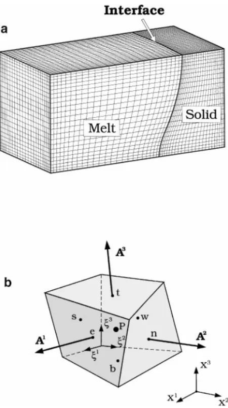
The physical problem can be easily decomposed into a number of blocks for analysis. For example, two blocks are adopted for Fig. 1b: one is for the melt and one for the solid. As the complexity of the problem increases, more blocks are needed. Multiple blocks can also be used in the same media, like in the melt. In each block, the finite-volume method based on the structured mesh used in the previous report [8] is adopted. The grid at the block interface can be coherent or incoherent. Although the incoherent interface is more versatile for a complicated domain, its implementation is tedious. Therefore, in this study only the coherent interface is considered.
3.1. Coordinate Transformation
Due to the unknown and deformed interface shape h(x2, x3), structured body-fitted co-ordinates (ξ1, ξ2, ξ3) are adopted for each block. The algebraic coordinate transformation
for both melt and solid phases are performed as follows:
Melt x1= ¯ξ1(ξ1)h(ξ2, ξ3), (14) x2= ¯ξ2(ξ2)W/H, (15) x3= ¯ξ3(ξ3). (16) Solid x1 = h(ξ2, ξ3) + ¯ξ1(ξ1)(L/H − h(ξ2, ξ3)), (17) x2= ¯ξ2(ξ2)W/H, (18) x3= ¯ξ3(ξ3). (19)
FIG. 2. (a) A sample mesh and (b) a 3D finite-volume and labeling scheme.
Here ¯ξ1(ξ1), ¯ξ2(ξ2), and ¯ξ3(ξ3) are stretch functions ranging from 0 to 1 for adjusting grid distribution. A hyperbolic tangent function with the following form, for example, for
¯ ξ1, is used, ¯ ξ1(ξ1) = 0.5 · 1+ tanh µ B[(ξ1− 1)/(N ξ1− 1) − 0.5] 0.5B ¶¸ , (20)
where B is a stretch constant and Nξ1 the number of control volumes (CVs) in the ξ1
direction. The coordinate transformation defines the boundaries of the CVs. For example, the corner coordinates of each CV in physical space, as shown in Fig. 2a, are calculated according to the transformation. The cell faces can be represented by surface vectors, i.e.,
A1, A2, and A3. For convenience,1ξ1= 1ξ2= 1ξ3= 1, so the CVs in the computational domain (ξ1, ξ2, ξ3) have unit volume. In the implementation,ξ1,ξ2, andξ3are simply the
loop indices I , J , and K for the three coordinates. The values of variables in each CV are defined at its geometric center. Since some variables on boundaries are unknown, to make coding easier the CVs on the boundaries are also assigned, but their volume is zero. Grids highly stretched toward the boundaries can be obtained easily by simply increasing the stretch constant B.
TABLE I
Form of Governing Equations
∂ ∂ξi(Ciφ + Di) + J Sφ= 0 φ Ci Di Sφ 1 Ui 0 0 u1 Ui − Pr J ³ Bi j∂u1 ∂ξj+ A i jω j 1 ´ −A j 1 J ∂℘ ∂ξj u2 Ui − Pr J ³ Bi j∂u2 ∂ξj+ A i jω j 2 ´ −A j 2 J ∂℘ ∂ξj u3 Ui − Pr J ³ Bi j∂u3 ∂ξj+ A i jω j 3 ´ −A j 3 J ∂℘ ∂ξj θ Ui −1 J ³ Bi j ∂θ ∂ξj ´ 0 Note. Ui= Ai juj, Bi j= AikA j k, and ω j i= (∂uj/∂ξk)Aki. 3.2. Finite-Volume Integration
After the coordinate transformation, the governing equations can be rewritten in a general conservation-law form for each block in(ξ1, ξ2, ξ3) as
∂
∂ξi(Ciφ + Di) + J Sφ= 0, (21)
where
J = det|∂xi/∂ξj|.
The variableφ and its associated coefficients are listed in Table I. For the convenience of representation, tensor notation (summation on free indices) is adopted here. Also, in Table I,
Aij represents the xj component of the surface vector Ai (see Fig. 2b). More importantly, the driving forces due to pressure gradients and the buoyancy force F are combined and redefined through a new variable℘ as
∂℘ ∂ξj ≡ Fk ∂xk ∂ξj − ∂ P ∂ξj, (22)
where Fkis the kth component of the body force F; F≡ Pr Ra θe3. The advantages of using
this variable have been discussed in our previous report [8].
The finite-volume method simply integrates Eq. (21) over each CV in the computational domain (ξ1, ξ2, ξ3). In fact, the integration performed over the physical domain (x1, x2, x3)
is the same as that over the computational domain after coordinate transformation, and 1V = J. After the Gauss theorem is applied, the integration over each CV results in a flux balance equation,
Ie− Iw+ In− Is+ It− Ib+
Z
1VSφd V = 0, (23)
where Ii, i = (e, w, n, s, t, b), represents the fluxes of φ across the faces of the CV. Each of the fluxes Ii is made of two distinct parts, namely a convective contribution IiC(=Ciφ)
and a diffusive contribution IiD(=Di). Both IiCand I
D
i are approximated with the central difference scheme. A detailed implementation of this boundary condition and related dis-cussions can be found elsewhere [8]. It should be noticed that the FVM formulation for each block is the same. The interface between blocks is set up by equating the fluxes from both sides.
Furthermore, since the pressure variable does not appear explicitly in the continuity equation, the use of linearly interpolated velocity at the cell faces for collocated grids could lead to the velocity/pressure decoupling or the so-called checkerboard oscillation of pressure. In order to amend this, the idea of the Rhie–Chow momentum interpolation scheme [21] is adopted. In other words, the velocity values required for the continuity equation are interpolated from the momentum equations, rather than linearly from the adjacent nodal values. Furthermore, for incompressible flow, the pressure does not appear explicitly in the continuity equation and only the pressure gradient is meaningful. Therefore, the concept of the pressure correction scheme from the SIMPLE method [16] is adopted.
4. SOLUTION SCHEME
4.1. Strong Implicit Procedure
The approximation from the previous section leads to a general nonlinear form as
aφPφP− X
nb
aφnbφnb= Sφ1V, (24)
for variableφ, and φ = u1, u2, u3, P, and θ at every CV center for each block. A similar
formulation can also be obtained for the block interfaces. The strong implicit procedure (SIP) based on the incomplete LU decomposition [22] is then used to solve Eq. (24). To ensure the diagonal dominance, the deferred correction method [23] is also used. With the deferred correction, the central difference scheme is allowed for the convection terms for all of the cases considered here.
The assembly of Eq. (24) for all variables and all blocks leads to a sparse block matrix. In each block for each variable, there are 9 diagonals for 2D problems, and 19 diagonals for 3D problems. In addition to SIP, other techniques, like the Gauss–Siedel (GS) method or preconditioned conjugate gradient (PCG) [24] methods, can also be used. However, for memory and performance, the SIP is adopted for each block, and the global iteration is performed variablewise and blockwise. The performance is found satisfactory for coarse grids, but becomes poor as the grid is refined. In fact, to most of the iterative methods, the convergence becomes slower as the number of equations increases. The convergence rate is fast only at the initial stage of the iterations, and it degrades rapidly as the iteration proceeds further. As mentioned before, this is because only the short wavelength errors are smoothed out efficiently. The long wavelength errors are hard to remove in the fine grid.
4.2. Multigrid Methods
An efficient way of overcoming the difficulties of slow convergence is to use differ-ent meshes for iterations, i.e., the MG methods. The concept of MG is simple, but its implementation is quite tedious. Careful design of the data structure is crucial to a success-ful implementation. If a wide spectrum of the wavelength for errors can been seen from
different grids, the convergence is expected to be faster. Therefore, to implement MG for each block, we further adopt several grid levels (multilevel) for the MG acceleration. For simplicity, the finest grid, which describes the shape of each block most accurately, is set up first. After setting up the finest grid, as the level is down for one level, eight contiguous control volumes (the kid volumes) are coalesced into a larger finite volume (the parent vol-ume). From there, a simple parent–kid link-list data structure is then set up for computation. Furthermore, there are several approaches to performing MG iterations. Among them, the full approximation scheme (FAS) proposed by Brandt [25], which has been widely used [14, 15], is adopted here. Since the detailed description of FAS can be found elsewhere [25], only a brief description is presented here.
Let us take two grids (levels), the coarse grid (CG) and the fine grid (FG), as an example. During iteration, the FG formulation of Eq. (24) is rewritten in a matrix form,
Afφf = Sf, (25)
where Afis the coefficient matrix and Sfthe source term. Since the solution of Eq. (25) is
the most time consuming part, we only iterate it several times. After the iterations, say three nonlinear iterations, we can estimate the FG residual Rfby
Rf= Sf− Afφf. (26)
This residual is then passed to CG to get the defect Dc. The corresponding CG residial Rc
and solutionφcare estimated first by linear interpolation (the so-called restriction step),
Rc= IfcRf, (27)
φc= Ifcφf, (28)
where Ic
f is the restriction operator for interpolating the values from FG to CG. Since the
structure grids are used here, i.e., eight FG CVs are coalesced into a CG CV, the value on the CG is simply the volume-weighted average from the FG values. The defect on CG, Dc,
is then estimated by
Dc≡ Acφc− Sc+ Rc. (29)
Now, the next step is to get a solution on CG (φc) with this defect by solving
Acφc= Sc+ Dc. (30)
Since the solution on the CG is much cheaper than that on the FG, enough nonlinear iterations (but less than 20) are performed on the CG. After the solution is obtained, the correction value1φcis calculated by subtracting the old value interpolated from FG,φc,
i.e.,
1φc= φc− φc. (31)
The FG correction1φfis again obtained by interpolation,
where Icf is the prolongation operator for interpolating the values from CG to FG. Equations (31) and (32) are the so-called prolongation step. Linear interpolation is found to be adequate in this study. The solution on the FG is then updated by
φf = φfold+ 1φf. (33)
This new solution is used as a guess for Eq. (25) for further nonlinear iterations on FG. The MG iteration continues until the solution on the FG converges. Again, the MG acceleration is done block by block.
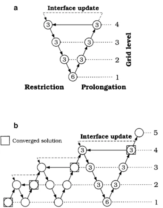
4.3. V-Cycle, FMG, and Interface Update
The MG procedure described above can be easily extended to more than two grids. Now, we must find the following: (1) a better MG procedure and (2) a better strategy for updating the interface. Two procedures for MG iterations are used here. With a known geometry, for each cycle, as illustrated in Fig. 3a, the procedure based on the previous section starts from the finest grid (top level) to the coarsest grid (lowest level) for restriction, and the prolonga-tion is from the lowest level upward to the top level. Because of its shape, it is also called the V-cycle scheme. After the fixed-geometry MG V-cycle iteration is converged, the interface update based on the isotherm migration method (IMM) [8] is performed on the top level, as shown by the dashed line with an arrow in Fig. 3a. The IMM is simply to locate the melting point isotherm by interpolation. After the interface shape is obtained, the grid is generated
using Eqs. (17)–(19) before entering the next fixed-grid V-cycle. The same procedure con-tinues until the residual for the interface update is reduced to an acceptable tolerance.
Since the initial guess is often far away from the final solution, it may make more sense to obtain a rough solution from the coarsest grid first. This is the original concept of FMG, as illustrated in Fig. 3b. As shown, the solution starts from the coarsest grid. After the solution is obtained, one (or more than one) grid level is added. The addition of the grid level continues until the top level is reached. The interface update can be added onto the top level like that used in the V-cycle. However, a more consistent way is to add it between levels, as shown by the dashed line with an arrow in Fig. 3b. In fact, FMG with the interface update can be seen as a combination of V-cycles with different levels.
There is an additional advantage of FMG. Since the solution is converged for each level of grids, the grid-independent solution can be obtained easily from different levels through Richardson extrapolation. As a result, the estimation of discretization errors and the order of convergence is possible after two levels of grids have been used. In other words, local mesh refinement may be implemented if a refinement tree is set up. Furthermore, since the solutions for coarser grids are only the initial guess for the finest grid, the convergence criteria can be looser. Therefore, another modification can be made by tightening up the convergence tolerance as the grid level goes up. Such a strategy can be used for both field and interface variables.
It should be pointed out that the IMM scheme can also be used for single-grid approaches somewhat differently. The interface is usually updated more frequently during iterations. For example, one could update the interface every 50 nonlinear iterations of the field vari-ables. Synchronized iterations can also be used by updating the interface right after each temperature iteration. However, such an interface update scheme is less stable because the isotherms are usually not smooth enough. Hence, it often requires underrelaxation. For example, one may use
hnew= hold+ α1h (34)
or
hnew = hold+ α(θ − 0), (35)
whereα is the relaxation parameter, but this does not force the interface temperature to be the melting point. Using the Stefan condition (Eq. (11)) is also a good way for single-grid methods to update the interface through its residual Rhby
hnew= hold+ αRh. (36)
However, the interface temperature has to be set at the melting point (θ = 0). Also, the synchronized iteration scheme is necessary to keep the interface shape stable.
5. RESULTS AND DISCUSSION
Since the performance of IMM relies on the convergence of fixed-grid calculations, the MG performance on the fixed-grid cases, as well as the benchmark comparison, is presented first in the next section. The applications of MG/IMM schemes will be presented in Section 5.2, followed by an example on the crystal growth application, where both buoyancy and thermocapillary flows are important, in Section 5.3.
5.1. Performance on Fixed-Boundary Problems
The performance on a 2D heated square problem [13, 26] for various Ra numbers (Pr = 0.71) is examined first; L/H = 1. Although Pr = 0.71 is usually used for air in the benchmark solution, for most oxides Pr is about the same order. Therefore, for the conve-nience of illustration, Pr= 0.71 is used throughout this report even for the cases with phase change unless otherwise stated. The no-slip boundary condition is used for all boundaries. The top and bottom walls are insulated, while the hot wall (θ = 1) is on the left and the cold wall (θ = 0) is on the right. For both single-grid (SG) and MG, u1= u2= P = θ = 0
is used as the initial guess. Five levels of meshes, from 10× 10 to 160 × 160, are used. For RaT= 105, less than 50 fine-grid iterations are used for both V-cycle MG and FMG
to achieve a normalized residual norm of 10−7. Using the finest grid alone, it will take more than 1000 iterations to reach a residual norm of only 10−2. The calculated Nu are in excellent agreement, up to four to five digits, with the benchmark results [13, 15, 27] for Ra= 104to 106. The cases with a 45◦skewed parallelogram are also conducted, which are
based on nonorthogonal grids and Pr= 0.1 or 10. Excellent agreement is obtained as well. The CPU time required for MG methods is linearly proportional to the number of equations (NEQ); i.e., CPU time∝ NEQn, n ∼ 1. For the single-grid approach, n ∼ 1.8, while n ∼ 1.6 for Newton’s method [8] using the ILU(0) preconditioned GMRES iterative matrix solver [28, 29], and the dimension of the Krylov subspace is 50. Due to the small convergence radius, for Newton’s method the solution at Ra= 104needs to be used as an initial guess for higher Ra. Furthermore, for all of the methods, the memory required is about linearly pro-portional to NEQ, but the memory required for MG is still much less than that for Newton’s method. More importantly, the CPU time required for NEQ= 140,000 is less than 50 s for one calculation on an IBM/590 workstation, which is one to two orders of magnitude faster than that by the single-grid solution as well as Newton’s method. The memory required is only 30 Mbytes.
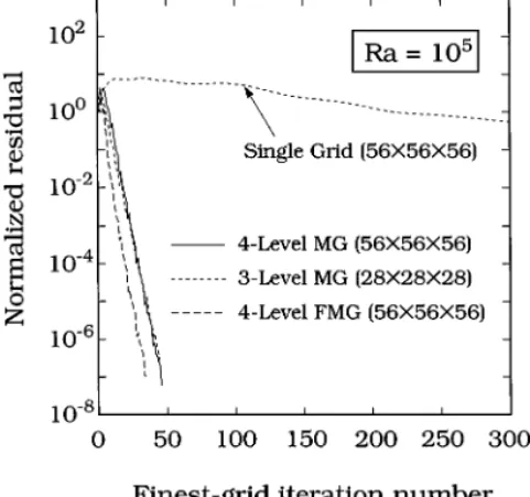
The convergence for a 3D heated box problem (L/H = 1 and W/H = 1) using a similar initial guess is illustrated in Fig. 4. As shown, the convergence of MG still outperforms that
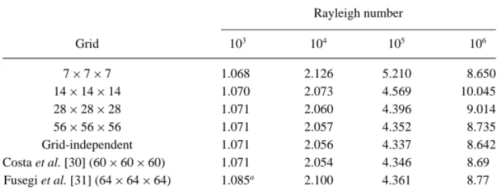
TABLE II Rayleigh number Grid 103 104 105 106 7× 7 × 7 1.068 2.126 5.210 8.650 14× 14 × 14 1.070 2.073 4.569 10.045 28× 28 × 28 1.071 2.060 4.396 9.014 56× 56 × 56 1.071 2.057 4.352 8.735 Grid-independent 1.071 2.056 4.337 8.642 Costa et al. [30] (60× 60 × 60) 1.071 2.054 4.346 8.69 Fusegi et al. [31] (64× 64 × 64) 1.085a 2.100 4.361 8.77 aThis result of Fusegi et al. for Ra= 103was obtained with a nonuniform grid of 32× 32 × 32.
of the single-grid method. Again, the convergence of MG is not affected by the problem size; the convergence rate for three and four levels is almost the same. Furthermore, the FMG seems to work better than the V-cycle MG. Clearly, for FMG, by the time the finest grid is added, its initial guess is good already even though the convergence rate remains the same. Furthermore, the benchmark comparison with previous calculations [30, 31] for
Nu is illustrated in Table II. Again, the agreement is very good, but our results are closer to
those by Costa et al. [30].
The flow patterns and isotherms calculated for the two-block case for Ra= 105are shown in Fig. 5. Due to the side wall insulation, the flow is quite similar to 2D flow; the flow in the third dimension is weak. In addition, since the interface is no longer at a fixed temperature, the flow is slightly different from that in a heated box. The comparison of CPU time required for different methods is summarized in Fig. 6, and again FMG appears to be the best method. Due to memory limitation, Newton’s method is excluded from the comparison for 3D calculations. For NEQ≈ 106, the FMG takes about 10 min CPU time on an IBM
workstation, and it is about two orders of magnitude faster than using the finest grid alone. 5.2. Performance on Free-Interface Problems
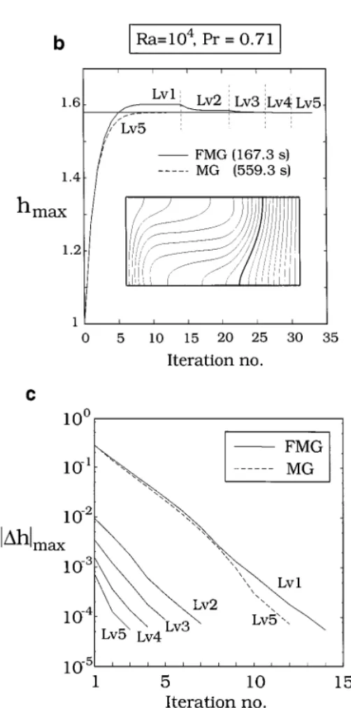
After the MG methods for the fixed-interface problems have been demonstrated, we are now ready to move on to the calculations including an unknown interface. When the melt/solid interface is included, the strategies on locating the interface are important. Figure 7a illustrates the IMM convergence of the interface shape (Ra= 104) by the V-cycle
MG; the MG/IMM iteration scheme is shown in Fig. 3a. As shown, it requires more than 5 fixed-grid iterations to converge; the initial guess is the same as before and h= 1. However, if we monitor the maximum interface position at x2= 1 during iterations, as shown by the dashed line in Fig. 7b, 10 iterations are needed to converge. Nevertheless, the final interface position is quite far away from the initial guess, which also illustrates the robustness of the IMM scheme here. The convergence of|1h|maxis further illustrated in Fig. 7c. Fourteen
interface updates are needed to reduce the norm to 10−4 for the V-cycle MG (again, the dashed line). Nevertheless, the number of fine-grid iterations for each interface shape is also significantly reduced as convergence is approached. As a result, the overall CPU time required is much less than that for 14 fixed-grid calculations. If Ra= 105is used, the inter-face position will move toward the cold wall even more. The CPU time required will be a bit more as well.
FIG. 5. Calculated temperature and velocity fields for the 3D two-block problem at Ra= 105.
FIG. 7. Multigrid methods for the 2D free-interface problem(Ra = 104): (a) interface update using the V-cycle
method (Fig. 3a); (b) convergence of the maximum interface position for V-cycle (dashed line) and FMG (the scheme is shown in Fig. 3b); and (c) convergence of interface corrections for V-cycle and each level of FMG. The converged isotherms are also shown in (b).
For FMG, the convergence of the maximum interface position is also shown in Fig. 7b (solid lines). Apparently, the convergence of the interface improves progressively as the grid level increases. Clearly, it takes much more interface updates, but mainly on the coarser meshes (lower levels). As the finest level is added, only two to four iterations are required to achieve the same accuracy as that by the V-cycle MG/IMM. As a result, the CPU time for FMG/IMM is only about one-third of that for the V-cycle MG/IMM. The difference can be further illustrated in Fig. 7c for the convergence history of the interface norm|1h|max
for both methods. Interestingly, the convergence rate for the interface using IMM seems to be the same for all levels of meshes; it converges almost linearly. In other words, the major difference between the V-cycle MG/IMM and FMG/IMM is the initial guess of the interface shape for the finest grid that requires most of the CPU time. As shown in Fig. 7c, for FMG, by the time the finest level is added, the initial norm|1h|maxis small already. As a result,
for the problem with an unknown interface shape, FMG/IMM requires about three times more CPU time than that needed for a fixed-grid problem. Furthermore, the convergence of the FG iterations is progressively speeded up due to the better initial guess from previous solutions. Therefore, the overall performance leads to the CPU time being less than three times of that for a fixed-grid problem.
Although the FMG/IMM scheme seems to be satisfactory, further improvement is still possible. By examining Fig. 7c, it is interesting to note that|1h|max always has a jump
from one grid level to the other due to interpolation. We also observe that the magnitude of the jump is not affected much by the convergence of the previous level if the convergence of the previous level is down to a certain degree (usually about a two-order decrease in the residual norm). Therefore, the convergence criteria for coarser grids for both field and interface variables can be loosened. By doing so, we can further reduce the CPU time by 15 to 30% for most cases.
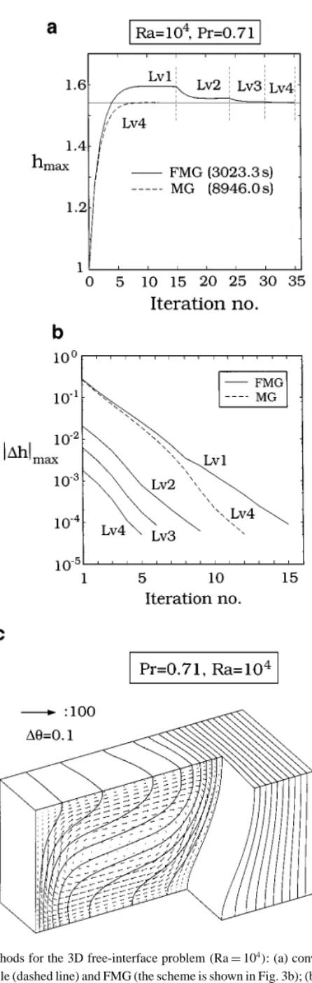
Similar convergence is also obtained for the 3D heated box problem with an interface (Ra= 104). The results are summarized in Fig. 8. As shown in Fig. 8a, the V-cycle MG/IMM is still about three times slower than the FMG/IMM. Although the FMG/IMM still requires about four fixed-grid iterations, the total CPU time for about one million unknowns is less than 50 min on an IBM RS6000/590 workstation with a good quality of convergence. The convergence rates of the interface at different levels by FMG, again, are very similar to those of the 2D case, as shown in Fig. 8b. The converged result for temperature and velocity fields is shown in Fig. 8c.
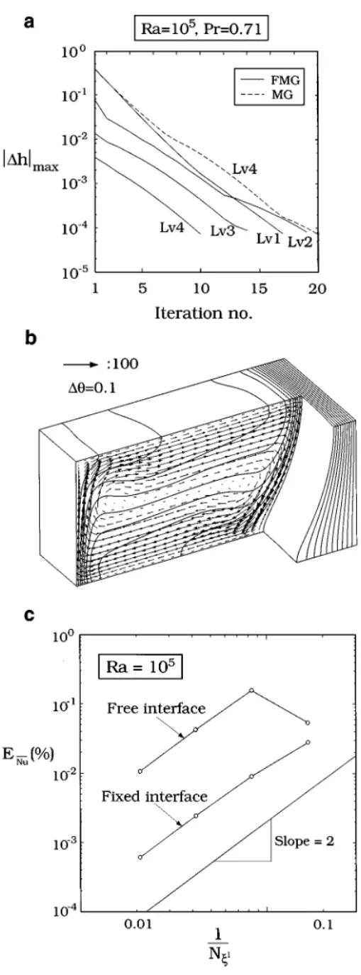
For a further illustration on the robustness and the convergence speed, the result for Ra= 105is placed in Fig. 9 for comparison; h= 1 and zero velocity and pressure are also
used for the initial guess. As shown in Fig. 9a, it requires more interface updates for both MG and FMG. The convergence rate is also slightly slower than that in the previous case. However, due to the much stronger flow, the interface position is farther away from the initial position and the isotherms become much more distorted. Even for single-grid calculations, the convergence for higher Ra is slower as well. In other words, the speedup of the MG schemes remains satisfactory. More importantly, when using the single-grid approach with the finest grid, it is difficult to achieve the same convergence criteria. Furthermore, since the side walls for the previous cases are insulated, the interface deformation in the third dimension is not much. A more deformed interface will be illustrated in Section 5.3 for crystal growth applications.
Since different levels of grids are used, the order of convergence can be estimated easily. The grid-independent solution is again obtained by Richardson extrapolation from the
FIG. 8. Multigrid methods for the 3D free-interface problem(Ra = 104): (a) convergence of the maximum
interface position for V-cycle (dashed line) and FMG (the scheme is shown in Fig. 3b); (b) convergence of interface corrections for V-cycle and each level of FMG; and (c) converged isotherms and velocity fields.
FIG. 9. Multigrid methods for the 3D free-interface problem(Ra = 105): (a) convergence of interface
correc-tions for V-cycle and each level of FMG; (b) converged isotherms and velocity fields; and (c) estimated errors of Nu as a function of grid size for the 3D fixed-grid and free-interface problems.
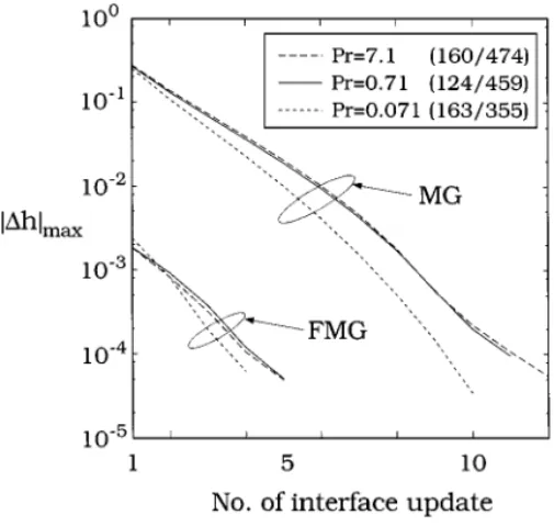
FIG. 10. Effects of Prandtl number (Pr) on the interface convergence of the V-cycle MG and FMG; only the finest grid results are shown. The numbers of finest grid iterations of FMG and V-cycle MG are indicated in parentheses in the legend.
solutions of the finest two grids. For the results in Figs. 5 and 9b, the error on Nu, i.e., ENu, as a function of grid spacing on the computational domain is plotted in Fig. 9c. As shown, as the grid is fine enough, second-order accuracy for both cases is obtained. Apparently, our FVM approximation is second-order accurate and it is the same as we did before for the 2D problems solved by Newton’s method [8].
Since the heat transfer and fluid flow are strongly coupled in our study, the Prandtl number can also affect the convergence. The convective heat transfer becomes more important with the increasing Prandtl number; the interface deformation is increased as well. To illustrate this, we use Ra= 104, and the effects of different Prandtl numbers on the interface
convergence and the total number of finest grid iterations for MG and FMG are shown in Fig. 10. As shown, for the interface update, the lower the Prandtl number, the faster the convergence speed. However, we are also aware that the convergence of the field variables, especially the velocity, slightly decreases as the Prandtl number increases. As a result, the total fine-grid iteration, and thus the CPU time, is not affected much by the Prandtl number.
5.3. Application to Crystal Growth
In previous calculations, we have demonstrated the convergence and robustness of the MG/IMM schemes, and the FMG/IMM has proven to be the most effective. The final example is to apply the FMG/IMM scheme to the HB crystal growth (Fig. 1c). As mentioned previously, the HB method is one of the major processes for growing GaAs single crystals for optoelectronic devices. The control of the growth interface has been of major interest to crystal growers because it directly controls the crystal quality. However, because the problem is 3D and the interface shape is unknown and strongly affected by the heat flow, both buoyancy and thermocapillary flows, its modeling is regarded as a great challenge in the crystal growth community. The first 3D coupled solution for the open boat configuration was conducted in our previous paper [19] using a SG/SIMPLE approach. The slow convergence
FIG. 11. Sample calculated results for the horizontal Bridgman crystal growth: (a) conduction mode(Ra = Ma= 0); (b) buoyancy mode (Ra = 104, Ma = 0); and (c) buoyancy and thermocapillary modes (Ra = 104,
Ma= 103). The interface shapes are also shown on the right-hand side for comparison; for clarity of
illustra-tion, the results are based on the grid level 3(196 × 34 × 34).
of the method for fine grids thus motivates the development of the present methods. To simplify the calculation, the crucible is neglected here; in practice, the crucible is very thin. The aspect ratios L/H = 8 and W/H = 2 are now much larger. Also, the thermocapillary convection is considered (Ma= 103). Crystal growth rate (Pe= 10−2), the heat of fusion
(St= 20), and the heat exchange with the environment (Bi = 5) are also included. A linear heating profile (in the x1direction) is imposed for the environment. Again, Pr= 0.71 is also
used.
The calculated results are shown in Fig. 11. For the case without convection in Fig. 11a, the isotherms and the interface shape are not deformed much; the interface shape is also plotted on the right of the figure for comparison. As the buoyancy force (Ra= 104) is considered in Fig. 11b, due to the flow the isotherms become quite distorted. As shown, the interface deformation in the x2 direction increases. As the Marangoni convection is taken into account (Ma= 103) in Fig. 11c, the velocity at the surface becomes much larger due to
the thermocapillary force. As a result, the interface deformation increases. Since the driving force for the flow at the free surface is proportional to the thermal gradients there, the flow near the crucible is driven outward; the velocity vectors are more or less perpendicular to the isotherms at the interface. As a result, near the crucible, the interface shape is sharpened by the flow. In fact, such a small contact angle could induce parasitic nucleation and results in a polycrystalline growth. The convergence of this example is still very good, which will be illustrated shortly. Therefore, the schemes presented here seem to be promising for crystal growth applications as well as for other solidification problems.
FIG. 12. Convergence of the maximum interface position for different convection modes using FMG for Fig. 11.
Furthermore, the performance of the interface update also depends on the convection modes. As shown in Fig. 12, the case with both flow modes takes the most interface updates for convergence because its solution is the farthest away from the initial guess. Even so, the number of interface updates for the top level ranges only from 5 to 10, which is still quite satisfactory. On the contrary, using the finest grid alone for Fig. 11c, the convergence is very slow. A comparison of their convergence is shown in Fig. 13, where we represent the convergence of the maximum interface position as a function of the number of fine-grid
FIG. 13. Comparison of the interface convergence for FMG and single-grid methods for Fig. 11c. SG-2 updates the interface synchronically with the field variables using Eq. (35) withα = 0.1.
iterations. As shown, FMG takes about 350 fine-grid iterations for convergence, while the single-grid methods take more than 3000 iterations. In fact, to make the comparison possible, the convergence criteria for the single-grid iterations are also loosened to about 0.01 for both field and interface variables. Two interface migration schemes are used for single-grid iterations. One updates the interface every 100 iterations of the field variables. The other updates the interface synchronically with the field variables, which requires a relaxation parameter of 0.1 to ensure the stability; see also Eq. (35). Through this comparison, it is clear that FMG outperforms the traditional single-grid approaches. The method is not only efficient, but also robust in crystal growth calculations.
6. CONCLUSIONS
Efficient multigrid methods are presented for solving 2D and 3D incompressible flow problems with an unknown melt/solid interface, mainly for solidification applications. The implementation concept is based on a multiblock and multilevel approach that allows com-plicated geometry of the problem to be treated. The present schemes are one to two orders of magnitudes faster than the global Newton’s method using the GMRES iterative matrix solver and the single-grid SIMPLE method. The CPU time required for the present schemes is linearly proportional to the problem size. Both V-cycle and full multigrid methods are tested for calculating the interface shape using the isotherm migration method. It is found that the full multigrid method is the most effective, and its best performance requires about two to three times more CPU time than is needed for a similar fixed-grid problem. The 2D and 3D cases with strong buoyancy convection are successfully tested on a workstation with good quality of convergence. The performance of the scheme is not affected much by the Prandtl number. Although the convergence for stronger flows is slower, its speedup is not degraded much in our study as long as the coarsest grid remains stable during iterations. The application to a 3D crystal growth problem with buoyancy and thermocapillary flows is further illustrated, and the present schemes outperform the traditional schemes. In principle, the present schemes may be easily extended to time-dependent problems as well as to other free-boundary problems. Local refinement may also be another extension.
ACKNOWLEDGMENTS
The authors are grateful for the support from the National Science Council and the National Center for High Performance Computing of the Republic of China under Grant NSC87-2214-E002-035.
REFERENCES
1. J. Chang and R. A. Brown, Natural convection in steady solidification: Finite element analysis of a two-phase Rayleigh–Benard problem, J. Comput. Phys. 53, 1 (1984).
2. C. J. Kim and M. Kaviany, Numerical method for phase change problems with convection and diffusion, Int. J. Heat Mass Transfer 35, 457 (1992).
3. M. Lacroix, Predictions of natural-convection-dominated phase-change problems by the vorticity–velocity formulation of the Navier–Stokes equations, Numer. Heat Transfer 22, 79 (1992).
4. R. Viswanath and Y. Jaluria, Computation of different solution methodologies for melting and solidification problems in enclosures, Numer. Heat Transfer, Part B 24, 77 (1993).
5. S. K. Sinha, T. Sundararajan, and V. K. Garg, Study of the effects of macrosegregation and buoyancy-driven flow in binary mixture solidification, Int. J. Heat Mass Transfer 36, 2349 (1993).
6. J. C. Chen, C. F. Chu, and W. F. Ueng, Thermocapillary convection and melt–solid interface in the floating zone, Int. J. Heat Mass Transfer 37, 1733 (1994).
7. C. W. Lan, Newton’s method for solving heat transfer, fluid flow and interface shapes in a floating molten zone, Int. J. Numer. Methods Fluids 19, 41 (1994).
8. M. C. Liang and C. W. Lan, A finite-volume/Newton method for a two-phase heat flow problem using primitive variables and collocated grids, J. Comput. Phys. 127, 330 (1996).
9. A. Iserles, A First Course in the Numerical Analysis of Differential Equations (Cambridge Univ. Press, Cambridge, 1996), p. 227.
10. W. Hackbusch, Multi-grid Methods and Applications (Springer-Verlag, Berlin, 1985).
11. S. P. Vanka, Block-implicit multigrid solution of Navier–Stokes equations in primitive variables, J. Comput. Phys. 65, 138 (1986).
12. W. Hackbusch and U. Trottenberg (Eds.), Proceedings, Third European Multigrid Conference (Birkhausen, Basel, 1991).
13. I. Demirdzic, Z. Lilek, and M. Peric, Fluid flow and heat transfer problem for non-orthogonal grids: Benchmark solution, Int. J. Numer. Methods Fluids 15, 329 (1992).
14. Z. Lilek, S. Muzaferija, and M. Peric, Efficiency and accuracy aspects of a full-multigrid simple algorithm for three-dimensional flows, Numer. Heat Transfer, Part B 31, 23 (1997).
15. J. Farmer, L. Martinelli, and A. Jameson, Fast multigrid method for solving imcompressible hydrodynamic problems with free interfaces, AIAA J. 32, 1175 (1994).
16. S. V. Patankar, Numerical Heat Transfer and Fluid Flow (Hemisphere, Washington, DC, 1980).
17. E. Monberg, in Handbook of Crystal Growth 2a: Basic Techniques, edited by D. T. J. Hurle (North-Holland, Amsterdam, 1994), p. 52.
18. M. C. Liang and C. W. Lan, Three-dimensional convection and solute segregation in vertical Bridgman crystal growth, J. Cryst. Growth 167, 320 (1996).
19. M. C. Liang and C. W. Lan, Three-dimensional thermocapillary and buoyancy convections and interface shapes in horizontal Bridgman crystal growth, J. Cryst. Growth 180, 587 (1997).
20. L. D. Landau and E. M. Lifshitz, Fluid Mechanics (Pergamon Press, Elmsford, NY, 1987), 2nd ed., Vol. 6, p. 217.
21. C. M. Rhie and W. L. Chow, Numerical study of the turbulent flow past an airfoil with trailing edge separation, AIAA J. 21, 1527 (1983).
22. H. L. Stone, Iterative solution of implicit approximations of multidimensional partial differential equations, SIAM J. Numer. Anal. 5, 530 (1968).
23. P. K. Khosla and S. G. Rubin, A diagonally dominant second-order accurate implicit scheme, Comput. Fluids
2, 207 (1974).
24. J. H. Ferziger and M. Peric, Computational Methods for Fluid Dynamics (Springer-Verlag, Berlin, 1996). 25. A. Brandt, Multilevel adaptive computations in fluid dynamics, AIAA Paper 79, 1455 (1979).
26. G. De Vahl Davis, Natural convection of air in a square cavity: A bench mark numerical solution, Int. J. Numer. Methods Fluids 3, 249 (1983).
27. M. Hortmann, M. Peric, and G. Scheuerer, Finite volume multigrid prediction of laminar natural convection: Bench-mark solutions, Int. J. Numer. Methods Fluids 11, 189 (1990).
28. J. A. Meijerink and H. A. van der Vorst, An iterative solution method for linear systems of which the coefficient matrix is a symmetric M-matrix, Math. Comput. 31, 148 (1977).
29. Y. Saad and M. H. Schultz, GMRES: A generalized minimal residual algorithm for solving nonsymmetric linear systems, SIAM J. Sci. Stat. Comput. 7, 856 (1986).
30. M. Costa, A. Oliva, and C. D. Perez-Segarra, Three-dimensional numerical study of melting inside an isother-mal horizontal cylinder, Numer. Heat Transfer, Part A 32, 531 (1997).
31. T. Fusegi, J. M. Hyun, K. Kuwaharas, and B. Farouk, A numerical study of three-dimensional natural con-vection in a differential heated cubical enclosure, Int. J. Heat Mass Transfer 34, 1543 (1991).