網路搜尋量是否可以增進股票市場波動率的預測?國際實證

(1)

國立臺灣大學管理學院財務金融學系碩士論文

Department of Finance College of Management

National Taiwan University Master Thesis

網路搜尋量是否可以增進股票市場波動率的預測?

國際實證

Can internet search volume improve volatility

forecasting for the stock markets? International Evidence

陳蕙妤 Hui-Yu Chen

指導教授：王耀輝博士 Advisor: Yaw-Huei Wang, Ph.D.

中華民國 101 年 6 月 June 2012

(2)

I

(3)

II

誌謝

回顧過去兩年研究所生涯，要感謝許多人的支持、鼓勵與幫助。首先要感謝家人在我就學期間的付出，謝謝父母不論是在物質上，還是在精神上的資助與支持，也謝謝妹妹總是在我心情煩躁時聽我抱怨。

對於論文的完成，最需要感謝的人莫過於指導教授─王耀輝老師，謝謝老師細心地教導和耐心地指導，總是能及時發現錯誤，並且在我遇到問題時提供解決方法，讓我得以順利克服論文所遇到的所有困難。也謝謝兩位口委老師─張森林老師和徐之強老師對論文的指正與建議，使得我的論文更佳的完善。

感謝所有財金所的同學們，和你們一起分享經驗、討論問題總讓我獲益良多。

尤其要謝謝恩偉、彥銘和宣叡給了我許多幫助，和你們在同一個指導老師門下感到很幸運。謝謝怡婷、佩汝和智閎總是耐心且不遺餘力地回答我的疑問，給我許多有用的建議。最後則要謝謝我的朋友們常常關心我、鼓勵我，偶而還要當我的垃圾桶。特別要謝謝相伊花了許多時間幫忙我檢查英文文法，讓我能及時訂正完論文。

此論文的完成，代表我的學生生涯告一個段落，我即將邁入職場，走向人生另一個階段。我將會持續地學習、充實自己，踏實地往人生目標邁進！

(4)

III

摘要

在這篇論文中，我們使用 Google 搜尋量作為測量散戶投資者注意的媒介，來探討在不同的國家中，搜尋量和股票市場波動率之間的動態關係，以及檢驗搜尋量是否可以幫助預測波動率。我們發現搜尋量對預測未來實現波動率(realized volatility)一般是有用的。當有一個正的搜尋量衝擊，波動率並不會立即的反應而是在之後有正向的移動，但是波動率卻可以立即地影響搜尋量。當建立波動率預測的模型，搜尋量增加了有價值的信息，並且正面地影響未來的波動率。它還可以顯著地增進預測波動率的預測能力在樣本內，樣本外也可以但比較不顯著。在新興市場(emerging markets) 和新領域市場(frontier markets)，搜尋量可以增進預測波動率的現象變得較不明顯。而在我們的實證當中，有些國家沒有這個現象的可能原因除了市場的開發程度，還有較低頻率的資料、意義較不明確單一的搜尋關鍵字、較低的 Google 市佔率、國家的所在位置、較低的網路使用者普及率和較低的散戶投資者的比例。

關鍵字: 實現波動率, 預測, 散戶投資者, 網路搜尋量

(5)

IV

Abstract

In this paper, we use Google search volume as proxy of retail investors’ attention to study the dynamic relationship with stock market volatility and examine if it can help to forecast volatility in different countries. We find search volume is useful to predict future realized volatility generally. When there is a positive shock of search volume, realized volatility wouldn’t react immediately but have positive movement later, while volatility can affect search volume immediately. Search volume adds valuable information for modeling volatility and influences future volatility positively. Search volume also can improve volatility forecasting in- and out-of-sample. But it becomes much more insignificantly in out-of-sample forecast evaluation. The phenomenon that search volume can improve volatility forecasting becomes more unobvious when turning to emerging markets and frontier markets. Besides the developed level of markets, there are some possible reasons, like lower frequency of data, less univocal search terms, lower market shares of Google, locations of countries, smaller penetration rate of internet users and lesser market shares of retail investors, can explain why this phenomenon becomes unobvious for some countries from our empirical results.

Key words: realized volatility, forecasting, retail investor, internet search volume

(6)

Contents

誌謝 ... II 摘要 ... III ABSTRACT ... IV

1. INTRODUCTION ... 1

2. DATA ... 6

2.1STOCK INDEX VOLATILITY ... 6

2.2INTERNET SEARCH VOLUME ... 10

2.3SUMMARY STATISTICS ... 17

3. METHODS ... 27

3.1VECTOR AUTOREGRESSIVE MODEL (VAR MODEL) ... 27

3.1.1 Granger causality test ... 28

3.1.2 Impulse response function (IRF) ... 28

3.1.3 Variance decomposition ... 29

3.2REGRESSION MODELS ... 29

3.3VOLATILITY FORECASTS ... 30

4. EMPIRICAL RESULTS ... 32

4.1DYNAMICS OF SEARCH VOLUME AND VOLATILITY (VAR MODEL) ... 32

4.1.1 Whether search volume is useful in forecasting volatility? ... 33

4.1.2 How volatility reacts over time to shock of search volume and vice versa? ... 36

4.1.3 How much of volatility can be explained by search volume? ... 38

4.2WHETHER SEARCH VOLUME HAS VALUABLE INFORMATION FOR MODELING VOLATILITY? .... 40

4.3DOES SEARCH VOLUME HELP TO IMPROVE VOLATILITY FORECASTS? ... 43

4.3.1 In-sample forecast evaluation ... 43

4.3.2 Out-of-sample forecast evaluation ... 50

4.4WHY SEARCH VOLUME CAN’T HELP TO FORECASTING VOLATILITIES IN SOME COUNTRIES? ... 57

5. CONCLUSION ... 60

REFERENCE ... 62

(7)

1

1. Introduction

In this paper, we use Google search volume (Da, Engelberg and Gao (2011)) as proxy of retail investors’ attention to study the dynamic relationship with stock market volatility, test whether it can add more information for modeling volatility, examine if it can help to forecasting volatility in- and out-of-sample per country and compare these phenomenon in different markets.

In stock markets, huge movements catch investors’ eyes. The model of Lux and Marchesi (1999) implies that volatility triggers search activity. And Merton (1987) establishes that investor attention may be relevant for stock pricing and stock liquidity.

When the attention of investors increases, this may indicate trading activity increases.

Many paper document that retail trades can make stock prices move (Kumar and Lee (2006), Dorn, Huberman and Sengmueller (2008), Kaniel, Sear and Titman (2008), Hvidkjaer (2008)). And Foucault, Sraer and Thesmar (2011) prove that trading activities made by retail investors are positively related to volatility, which can be regarded as behaviors of noisy traders. They estimate that volatility is driven by retail investors about 23% except fundamentals. Therefore, abnormal volatility attracts retail investors’ attention and then causes retail investors invest in, which in turn makes volatility.

Nevertheless, measuring retail investors’ attention is a hard work since it cannot be observed directly. In empirical studies, many proxies for attention have been employed, like published news announcements and headlines (Mitchell and Mulherin (1994), Berry and Howe (1994), Frieder and Subrahmanyam (2005), Barber and Odean (2008) and Yuan (2008), Fang and Peress (2009)), trading volume (Gervais, Kaniel, and Mingelgrin (2001), Barber and Odean (2008), Hou, Peng, and Xiong (2008)), advertisement expense (Grullon, Kanatas, and Weston (2004), Lou (2008),

(8)

2

Chemmanur and Yan (2009)), price limits (Seasholes and Wu (2007)) and extreme returns (Barber and Odean (2008)). But using these proxies need critical assumption that if stock’s name is mentioned or its return or turnover is extreme, then that indicate retail investors must pay attention to it, while this assumption cannot be guarantee in practice.

Internet search volume is proved to be a more direct and easier method to measure retail attention by Da, Engelberg and Gao (2011), who use search volume of stock tickers from Google Trends. They show that this method is timelier than other well-established attention proxies and mainly captures the retail investor attention.

This method seems to be adequate for two reasons. First is that, nowadays, internet has become a popular way to search for information for individual investors. Since the usage of internet increased steadily worldwide during the recent decades, World Wide Web became accessible by nearly everyone and everywhere. And it is the largest pool which supply available information, freely or costly. Internet user usually choose search engine to seek information when needed. Second, an internet user will actively search a specific word only if he or she has interest in or demand for information about the object underlying the keyword.

Google search volume is the most popular proxy since Google search engine has the largest worldwide market shares, accounted for about 90.7% of all search engine on 2011.¹ Google search volume has significantly positive effects on trading activity, trading volume, stock liquidity and return volatility, both historical and implied (Vlastakis and Markellos (2010), Bank, Larch and Peter (2011)).

In addition, there are several evidences that internet search volume has power to forecast, such as unemployment rates, home sales, automotive sales (Choi and Varian

1 Source: StatCounter Global Stats (http://gs.statcounter.com/)

(9)

3

(2009)) and influenza (Ginsberg et al. (2009)). In the financial field, Google search volume is documented to predict earnings (Da et al (2010a), Drake, Roulstone and Thornock (2011)), abnormal returns and trading volumes (Joseph, Wintoki, Zhang (2011)). Da et al. (2011) report that an increase in Google search volume predict higher stock prices in the short-run and reversals in the long run, which is consist with the attention theory of Barber and Odean (2008).

Nowadays is the era of globalization. Investors use international portfolio to diversify risks and increase profits. Besides to invest in developed markets and emerging markets, more and more investors like to invest in frontier markets. It is proved that when portfolio contains equities of frontier markets, both portfolio risk and returns can be improved (Jayasuriya and Shambora (2009)). In this point of view, we want to comprehensively explore not only the relationship between retail investors’

attention measured by internet search volume and the stock market volatility but also the predict power of search volume for volatility forecasting in different markets with different development levels.

From the view of international portfolio, we’d like to use the same internet search engine, Google search volume index, measuring worldwide attentions of retail investors for three different MSCI indices, developed, emerging and frontier markets (DM, EM, FM) index, to test if search volume can increase different index volatility forecasting power. However, this method cannot be used since Datastream doesn’t provide these three MSCI indices’ intraday high and low prices, which are needed for realized volatility, and Google Trends also have not enough search volume data of MSCI frontier markets index.

Moreover, in stock markets, the main retail investors usually are local residents not foreigners. Instead, we focus on leading indices of each country, which belongs to

(10)

4

markets of various development levels according to MSCI Market Classification.² And we should choose the internet search volume whose search engine has the highest market shares in its home country to measure local attentions of retail investors. In almost countries, Google is the most popular search engine. Baidu and Naver is leading search engine in China and South Korea respectively. But there are problems that they either have no English version or do not provide detail search volume data to be downloaded. Therefore, we use Google search volume to measure local attentions for each country’s leading index and then test if search volume can improve volatility forecasting in different markets.

At first, we estimate a VAR model for every stock index to capture the dynamic relationship between Google search volume and stock index volatility. And then examine if past volatility can significantly influence present search volume (Granger (1969) and Sims (1972)) by Granger causality tests, see how volatility reacts over time to shock of search volume, and vice versa, by impulse response function and test how much of volatility can be explained by internet search volume by long-run variance decomposition under the VAR model. Next, we use three other regression models, AR(1), HAR and EGARCH, to rule out whether search volume has additional information for modeling volatility. Last, we compare the forecasting ability of the volatility models with and without lagged search volume in- and out-of-sample by using the mean squared error (MSE), the quasi-likelihood loss function (QL) and the R² of regression of the actual realized volatilities on their prediction.

We find past search volume is useful to predict future volatility generally and half of countries’ Granger causality is bi-directional: high search activities follow high volatility, and high volatility follows high search activities. But, when there is a

2 Source: http://www.msci.com/products/indices/market_classification.html

(11)

5

positive shock of search volume, volatility wouldn’t react immediately but have positive movement later while volatility can affect search volume immediately.

Throughout all countries, movement of volatility is contributed by search volume is ranging from 0.11% to 20.53%. As consistent with Foucault, Sraer and Thesmar (2011), search volume adds valuable information for modeling volatility and influences future volatility positively. Search volume also can improve volatility forecasting in- and out-of-sample. But it becomes much more insignificantly in out-of-sample forecast evaluation.

As the developed level of markets is lower, the phenomenon that search volume can help to forecast volatility becomes less obvious. Besides the developed level of markets, there are some possible reasons of why this phenomenon can’t be seen from our tests and models in some countries. The proper reasons are lower frequency of data, less univocal search terms, lower market shares of Google, location of countries, smaller penetration rate of internet users and lesser market shares of retail investors.

The remainder of this paper is organized as follows. In Section 2, we describe the search volume data, data set of realized volatility and the statistics. Section 3 explains the method, models and tests that we use where section 3.1 studies the dynamic relationship between Google search volume and stock index volatility, section 3.2 examine whether the search volume can add valuable information to different volatility models and section 3.3 evaluates in- and out-of-sample volatility forecasts to examine if search volume can help to forecast future volatility. Section 4 is the results of tests and modeling. Finally, section 5 concludes.

(12)

6

2. Data

2.1 Stock index volatility

This study presents an analysis across market classifications, developed, emerging and frontier. We select 24 developed countries, 21 emerging countries and 24 frontier countries according to MSCI Market Classification.

From Datastream, we download the daily close prices, intraday high prices and intraday low prices of main stock index per country from June 2004 to February 2012.

However, Datastream doesn’t provide all indices’ intraday high and low prices, especially for frontier markets, and some intraday high and low prices start from 2006/4/20 or later. Note that we use all three indices of USA since S&P 500, NASDAQ and DJIA are all important index in USA.

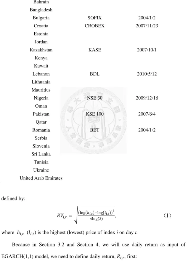
Table 1 contains the list of countries chosen from MSCI Market Classification, the name of leading index for each country and the start date of intraday high and low prices data provided by Datastream. For those countries without index name and start date mean that intraday high and low prices are not provided by Datastream. We will remove those countries without intraday high and low prices. For example, panel A shows that in developed markets, only New Zealand doesn’t have intraday high and low prices data. Panel B displays that 21 countries decrease to 16 countries in emerging markets. Panel C shows that in frontier markets, only 8 countries have intraday high and low prices data. Among these indices, the index price data of BDL, the leading index of Lebanon, has the shortest period starting from 2010/5/12.

Many researches use squared daily return as proxy for volatility. But any realized volatility measure calculated from only daily return will be noisy estimate. So we use the volatility proxy introduced by Parkinson (1980), which is much more accurate than the squared daily return. For stock index i, daily realized volatilities, _, , are

(13)

7

Table 1

List of countries with leading index and start date

This table displays the list of countries chosen from MSCI Market Classification, the name of leading index for each country and the start date of intraday high and low prices data provided by DataStream. For those countries without index name and start date mean that intraday high and low prices are not provided by DataStream. Panel A, B and C provide the list of developed, emerging and frontier markets respectively.Note that we use three leading indices, S&P 500, NASDAQ and DJIA, in USA.

Panel A: Developed Markets

Country Index Start Date

Australia S&P/ASX 200 2004/1/2

Austria ATX 2004/1/2

Belgium BEL 20 2004/1/2

Canada S&P/TSX COMPOSITE 2004/1/2 Denmark OMXC20 2004/1/2

Finland OMXH 2004/1/2

France CAC 40 2004/1/2

Germany DAX 30 2004/1/2

Greece ATHEX COMPOSITE 2004/1/2

Hong Kong HANG SENG 2004/1/2

Ireland ISEQ 2004/1/2

Israel TA 100 2006/4/20

Italy FTSE MIB 2004/1/2

Japan NIKKEI 225 2004/1/2

Netherlands AEX 2004/1/2

New Zealand

Norway OBX price 2004/1/2

Portugal PSI-20 2004/1/2

Singapore STRAITS TIMES 2008/1/15

Spain IGBM 2004/1/2 Sweden OMXS30 2004/1/2

Switzerland SMI 2004/1/2

United Kingdom FTSE 100 2004/1/2

USA S&P 500 2004/1/2

USA NSADAQ 2004/1/2 USA DJIA 2004/1/2

(14)

8

Table 1-Continued

Panel B: Emerging Markets

Brazil

Chile IGPA 2006/4/20

China SSE A SHARE 2004/1/2

Colombia IGBC 2004/1/2

Czech Republic Egypt

Hungary BUX 2004/1/2

India SENSEX 2004/1/2

Indonesia IDX COMPOSITE 2004/1/2

South Korea KOSPI 2004/1/2

Malaysia KLCI 2004/1/2

Mexico BOLSA 2004/1/2 Morocco

Peru IGBL 2006/4/20

Philippines PSEi 2004/1/2

Poland

Russia RTS 2004/1/2

South Africa FTSE/JSE ALL SHARE 2006/4/20

Taiwan TAIEX 2004/1/2

Thailand SET 2004/1/2

Turkey ISE 100 2006/4/20

(15)

9

Table 1-Continued Panel C: Frontier Markets

Argentina MERVAL 2004/1/2

Bahrain Bangladesh

Bulgaria SOFIX 2004/1/2

Croatia CROBEX 2007/11/23

Estonia Jordan

Kazakhstan KASE 2007/10/1 Kenya

Kuwait

Lebanon BDL 2010/5/12

Lithuania Mauritius

Nigeria NSE 30 2009/12/16

Oman

Pakistan KSE 100 2007/6/4

Qatar

Romania BET 2004/1/2 Serbia

Slovenia Sri Lanka

Tunisia Ukraine United Arab Emirates

defined by:

, ^, ^, , (1)

where _, ( _, ) is the highest (lowest) price of index i on day t.

Because in Section 3.2 and Section 4, we will use daily return as input of EGARCH(1,1) model, we need to define daily return, _, , first:

(16)

10

, log ^,

, , (2)

where _, is the close price of index i on day t.

Besides, we will use weekly search volume instead if daily search volume is not available for index. So we also have to define weekly realized volatility, _, , and weekly return, _, :

, ∑ _, , (3)

, log ^,

, , (4)

where t is Friday, t-4 is Monday and t-5 is last Friday.

2.2 Internet search volume

For internet search volume, we choose to use the search engine which has the highest market shares according to StatCounter Global Stats, which express global and each country’s ranking of search engines’ market shares. In global, Google has about 90.7% market shares of all search engines on 2011.

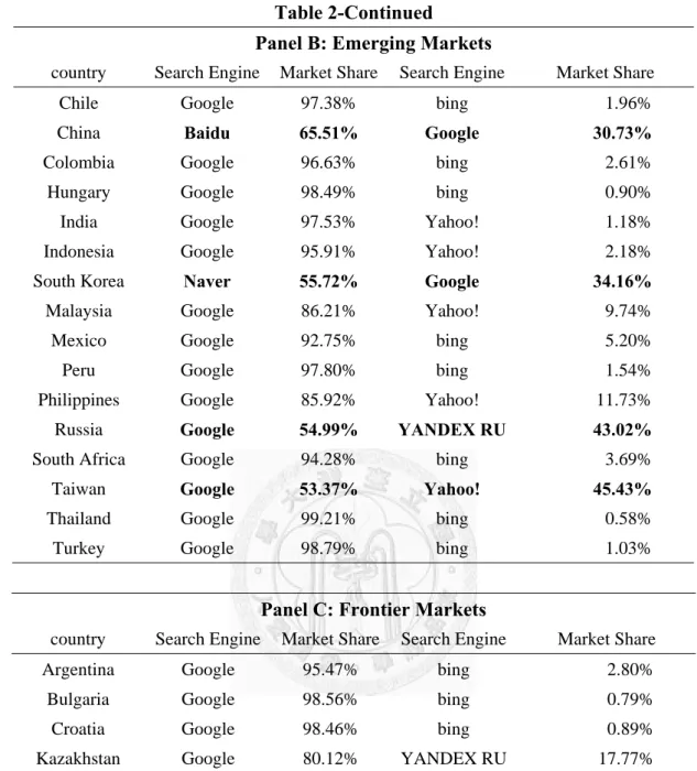
Table 2 presents top 2 search engines with market shares in each country on 2011.

Panel A, B and C are developed, emerging and frontier markets respectively. From this table we find that in addition to China, where Baidu is the biggest search engine, and South Korea, where Naver is the most popular search engine, Google has the highest market shares in the other countries. And the market shares of Google are beyond 70% in almost all countries, except Hong Kong, Russia and Taiwan, where market shares are between 53.37% and 59.60%. Although Google is not the top one in China and South Korea, it still owns 30.73% and 34.16% market shares respectively, ranked at second.

Eventually, we use the same search engine, Google, to measure local attention of individual investors. There are two main reasons. First is the problem of language,

(17)

11

Table 2

Top 2 search engines on 2011

This table presents top 2 search engines with market shares in each country on 2011. Data source is StatCounter Global Stats (http://gs.statcounter.com/). Panel A, B and C are developed, emerging and frontier markets respectively. The country whose top 1 search engine has market shares below 70% or is not Google is indicated through bold numbers.

Country Search Engine Market Share Search Engine Market Share

Australia Google 94.11% bing 3.92%

Austria Google 96.91% bing 1.98%

Belgium Google 98.08% bing 0.83%

Canada Google 91.83% bing 4.79%

Denmark Google 96.57% bing 2.62%

Finland Google 97.90% bing 1.68%

France Google 94.89% bing 2.99%

Germany Google 95.73% bing 1.99%

Greece Google 97.63% bing 1.56%

Hong Kong Google 59.60% Yahoo! 39.35%

Ireland Google 94.60% bing 2.71%

Israel Google 97.17% bing 1.87%

Italy Google 96.76% Yahoo! 1.07%

Japan Google 70.85% Yahoo! 26.65%

Netherlands Google 94.61% StartPagina 2.54%

Norway Google 93.77% bing 3.00%

Portugal Google 96.98% bing 1.95%

Singapore Google 85.91% Yahoo! 11.12%

Spain Google 96.48% bing 2.28%

Sweden Google 96.80% bing 2.41%

Switzerland Google 96.35% bing 2.28%

United Kingdom Google 91.78% bing 4.40%

USA Google 79.71% Yahoo! 9.57%

(18)

12

country Search Engine Market Share Search Engine Market Share

Chile Google 97.38% bing 1.96%

China Baidu 65.51% Google 30.73%

Colombia Google 96.63% bing 2.61%

Hungary Google 98.49% bing 0.90%

India Google 97.53% Yahoo! 1.18%

Indonesia Google 95.91% Yahoo! 2.18%

South Korea Naver 55.72% Google 34.16%

Malaysia Google 86.21% Yahoo! 9.74%

Mexico Google 92.75% bing 5.20%

Peru Google 97.80% bing 1.54%

Philippines Google 85.92% Yahoo! 11.73%

Russia Google 54.99% YANDEX RU 43.02%

South Africa Google 94.28% bing 3.69%

Taiwan Google 53.37% Yahoo! 45.43%

Thailand Google 99.21% bing 0.58%

Turkey Google 98.79% bing 1.03%

Panel C: Frontier Markets

country Search Engine Market Share Search Engine Market Share

Argentina Google 95.47% bing 2.80%

Bulgaria Google 98.56% bing 0.79%

Croatia Google 98.46% bing 0.89%

Kazakhstan Google 80.12% YANDEX RU 17.77%

Lebanon Google 94.58% bing 2.81%

Nigeria Google 88.96% Yahoo! 4.94%

Pakistan Google 94.67% Yahoo! 2.46%

Romania Google 97.62% Yahoo! 1.13%

like Naver, the top one search engine in South Korea, is all in Korean without the version of English. Next, search engine does not provide detail search volume data to be downloaded, ex: Yahoo!.

Google provide Search Volume index, instead of effective total number, of

(19)

13

search term publicly by Google Trends.³ This index is a portion of Google web searches to compute how many searches have been done for the terms we enter, relative to the total number of searches done on Google over time. In this website, we can see graph of search volume index and download the search volume data globally, or in specific region, country or city, even in different periods. We also can compare search volume of several searching terms, up to five, when entering terms separated by comma “,”.

After we signed into our Google Account, we could download two different modes of scaled data, relative and fixed. In relative mode, the data is scaled to the average search traffic for search term (represented as 1.0) during the time period we’ve selected while in fixed mode, the data is scaled to the average traffic during a fixed point in time (usually January 2004). Since the scale basis doesn’t change with time in fixed mode, we can relate them in different time periods. Therefore, we all download the search volume data with fixed scaling.

Search volume could date back to January 2004. We’d like to download the highest frequency search volume data, the daily data. But the search volume data at daily frequency may has many missing data, or even not enough volume to show graph and to be downloaded. For those indices with above problems, we will make use of weekly search volume instead. We only consider trading days of the stock markets in order to match search volumes to the respective time series of volatility.

A search engine user may search for a specific index using its name, ticker symbols or moreover, the short name of its stock exchange. Since stock indices often have many names and ticker symbols, it is a problem to choose an appropriate search term for stock index. We need to find the most widely used search term for specific

3 Source: http://www.google.com.tw/trends/.

(20)

14

stock index. In general, the short name of the index is preferred by individuals. Take the leading index, S&P/ASX 200, in Australia for example. Using its name as search term, there is not enough search volume to show graph. Search volume of “ASX 200”

has a lot missing data before 2011. Finally, we set “ASX”, which has correlation about 0.84 with “ASX 200” and far more often been searched, as keywords to download daily search volume data.⁴

For USA, we use all three leading index, S&P 500, NASDAQ, DJIA. The answer of the question which search term individuals use when looking for information about the stock index is easy, especially NASDAQ, which “NASDAQ” is used as keywords. For S&P 500, the number of search volume of “S&P” is about 2.1 times as often as the term “S&P 500”. The correlation between the two search terms is 0.84. To DJIA, search volume of “DJIA” and “Dow Jones” amount to 15% and 46%

respectively when compared to “Dow”. And the pairwise correlations between these search volumes are remarkably high, all above 0.96. Therefore, we choose the search term that is most preferred by retail investors.

However, for some countries, we cannot find search volume of index while using its names or ticker symbols. At this time, we choose to use the name or short name of stock exchange where the index is traded. For example, “Bolsa de Madrid” is the Spanish name of the stock exchange of the leading index, IGBM, in Spain. We take away those countries which we cannot discover any search volume of the main index.

And then we rearrange the sample period for each country. We also remove the countries whose number of observation is under 100, such as Portugal, whose search volume data has too many missing data before 2011.

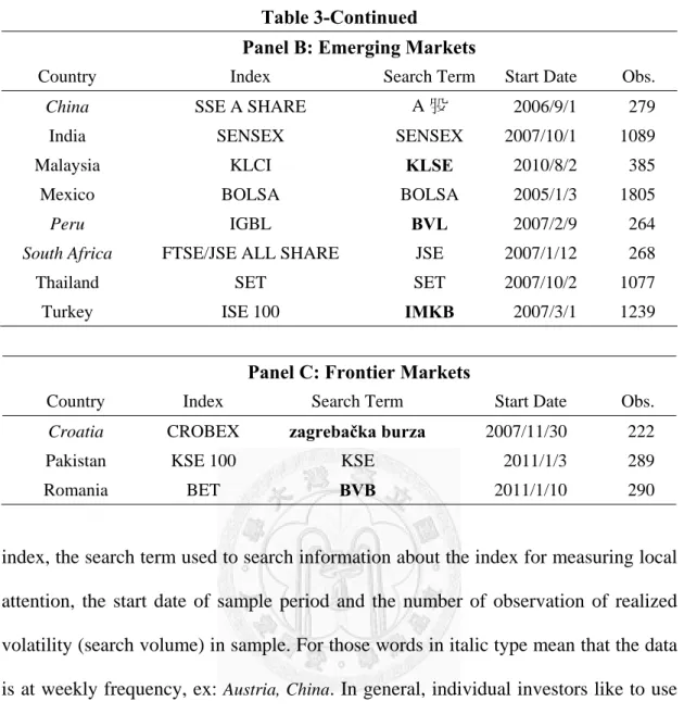
Table 3 displays the list of countries in our sample with the name of leading

4 Source: Google Correlate (http://www.google.com/trends/correlate/)

(21)

15

Table 3

List of countries in the sample with search term, start date and number of observation

This table contains the list of countries in our sample with the name of leading index, the search term used to measure local attention, the start date of sample period and the number of observation of realized volatility (search volume) in sample. For those name of countries in italic type mean that the data is at weekly frequency, ex: Austria. The search term which is not short name of relative index is indicated through bold type. Panel A, B and C provide the list of developed, emerging and frontier markets respectively.

Country Index Search Term Start date Obs.

Australia S&P/ASX 200 ASX 2005/7/7 1684

Austria ATX ATX 2008/9/19 180

Belgium BEL 20 BEL 2004/1/9 425

Canada S&P/TSX COMPOSITE TSX 2005/7/19 1661

France CAC 40 CAC 2007/1/2 1325

Germany DAX 30 DAX 2006/1/2 1571

Hong Kong HANG SENG HANG 2009/2/9 760

Italy FTSE MIB MIB 2007/8/31 224

Japan NIKKEI 225 NIKKEI 2005/11/1 1552

Netherlands AEX AEX 2007/1/2 1323

Singapore STRAITS TIMES STRAITS 2009/2/2 775 Spain IGBM Bolsa de Madrid 2006/10/2 1380

Sweden OMXS30 OMX 2009/8/14 133

Switzerland SMI SMI 2007/11/9 225

United Kingdom FTSE 100 FTSE 2006/1/3 1558

USA S&P 500 S&P 2006/1/3 1551

USA NASDAQ NASDAQ 2005/1/3 1803

USA DJIA DOW 2005/1/3 1803

(22)

16

Country Index Search Term Start Date Obs.

China SSE A SHARE A 股 2006/9/1 279

India SENSEX SENSEX 2007/10/1 1089

Malaysia KLCI KLSE 2010/8/2 385

Mexico BOLSA BOLSA 2005/1/3 1805

Peru IGBL BVL 2007/2/9 264

South Africa FTSE/JSE ALL SHARE JSE 2007/1/12 268

Thailand SET SET 2007/10/2 1077

Turkey ISE 100 IMKB 2007/3/1 1239

Country Index Search Term Start Date Obs.

Croatia CROBEX zagrebačka burza 2007/11/30 222

Pakistan KSE 100 KSE 2011/1/3 289

Romania BET BVB 2011/1/10 290

index, the search term used to search information about the index for measuring local attention, the start date of sample period and the number of observation of realized volatility (search volume) in sample. For those words in italic type mean that the data is at weekly frequency, ex: Austria, China. In general, individual investors like to use short name of index to search information. Only in Malaysia, people more prefer to use the ticker symbol. “KLSE” is one of ticker symbols of the leading index, KLCI, which we cannot find enough search volume of its short name. There are 6 countries, Spain, Sweden, Peru, Turkey, Croatia and Romania, where (short) names of stock exchange are used as search terms.

From Panel A of Table 3, there are 18 indices which belong to developed markets in our sample. Among these countries, there are 5 countries, Austria, Belgium, Italy, Sweden and Switzerland, which weekly data are used. The longest sample period is Belgium but the number of observation is only 425 since the data is at weekly

(23)

17

frequency. Panel B of Table 3 shows that 8 emerging countries are included in sample and weekly data are used for China, Peru and South Africa. The last panel of Table 3 presents that in frontier markets, only Croatia with weekly data and 2 countries with daily data are contained in sample.

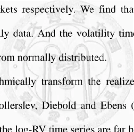
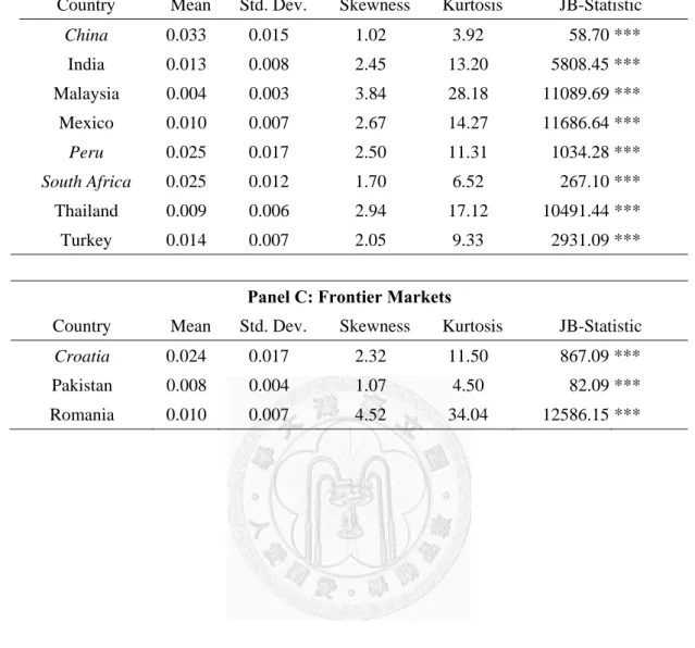
2.3 Summary statistics

Table 4 presents the descriptive statistics of realized volatility of each index, including mean, standard deviation, skewness, kurtosis and Jarque–Bera statistic (JB-Statistic), which is used to test the hypothesis that the data are from a normal distribution. A star, double star and triple star denote significance at 10%, 5% and 1%

level, respectively. Panel A, B and C provide the summary statistics of developed, emerging and frontier markets respectively. We find that weekly data have higher standard deviation than daily data. And the volatility time series per country are all positively skewed and far from normally distributed.

Therefore, we logarithmically transform the realized volatility time series as suggested by Andersen, Bollerslev, Diebold and Ebens (2001) and Andersen et al.

(2003). Table 5 shows that the log-RV time series are far better than RV data although log-RV time series mostly are not normally distributed.

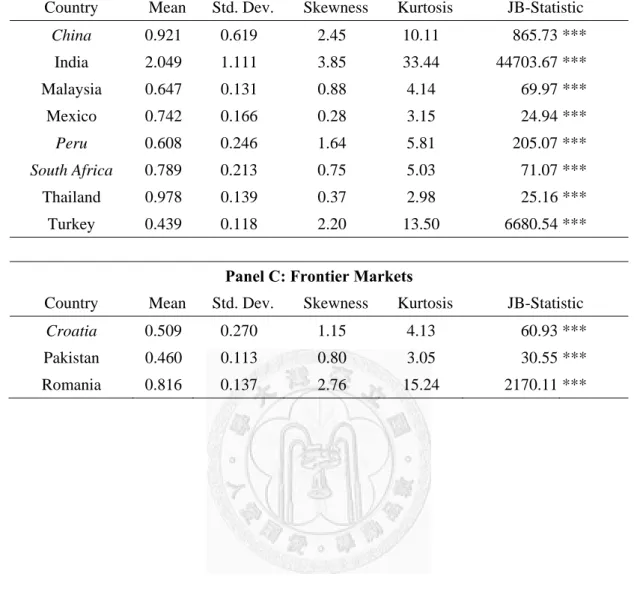
Table 6 displays the descriptive statistics of search volume (SV) of each index.

Just like the realized volatility data, the search volume time series are also heavily skewed and normality are all rejected with 99% confidence level. We therefore also take logarithms of search volume data (log-SV), whose descriptive statistics are showed by Table 7. Both skewness and excess kurtosis are significantly reduced, but normality is still rejected mostly.

Figure 1 displays the graphs of daily realized volatility (gray) and search volume (black) of the stock indices DJIA (USA), CAC 40 (France), SENSEX (India) and

(24)

18

Table 4

Summary statistics of realized volatility

This table presents the descriptive statistics of realized volatility of each index. Jarque–Bera statistic (JB-Statistic) is used to test null hypothesis that the data are from a normal distribution. For the name of countries in italic type mean that the data is at weekly frequency, ex: Austria. A star, double star and triple star denote significance at 10%, 5% and 1% level, respectively. Panel A, B and C provide the summary statistics of developed, emerging and frontier markets respectively.

Country Mean Std. Dev. Skewness Kurtosis JB-Statistic Australia 0.008 0.005 2.47 12.89 8564.19 ***

Austria 0.036 0.022 2.10 9.08 409.84 ***

Belgium 0.019 0.012 2.41 12.06 1866.21 ***

Canada 0.009 0.007 3.74 27.15 44197.68 ***

France 0.012 0.007 1.96 8.36 2433.92 ***

Germany 0.011 0.008 2.44 12.01 6861.55 ***

Hong Kong 0.009 0.005 1.57 7.09 841.62 ***

Italy 0.032 0.015 1.53 6.09 176.67 ***

Japan 0.009 0.007 4.22 32.25 59912.97 ***

Netherlands 0.011 0.007 2.22 9.98 3773.62 ***

Singapore 0.007 0.004 2.17 10.01 2190.80 ***

Spain 0.011 0.007 2.22 13.05 6932.78 ***

Sweden 0.024 0.011 1.80 8.18 220.28 ***

Switzerland 0.023 0.013 2.24 9.93 637.92 ***

United Kingdom 0.010 0.007 2.64 13.99 9645.66 ***

USA-S&P 500 0.010 0.008 2.97 15.74 12749.70 ***

USA-NASDAQ 0.009 0.007 2.99 16.65 16678.06 ***

USA-DJIA 0.009 0.007 3.40 20.53 26544.49 ***

(25)

19

Country Mean Std. Dev. Skewness Kurtosis JB-Statistic

China 0.033 0.015 1.02 3.92 58.70 ***

India 0.013 0.008 2.45 13.20 5808.45 ***

Malaysia 0.004 0.003 3.84 28.18 11089.69 ***

Mexico 0.010 0.007 2.67 14.27 11686.64 ***

Peru 0.025 0.017 2.50 11.31 1034.28 ***

South Africa 0.025 0.012 1.70 6.52 267.10 ***

Thailand 0.009 0.006 2.94 17.12 10491.44 ***

Turkey 0.014 0.007 2.05 9.33 2931.09 ***

Croatia 0.024 0.017 2.32 11.50 867.09 ***

Pakistan 0.008 0.004 1.07 4.50 82.09 ***

Romania 0.010 0.007 4.52 34.04 12586.15 ***

(26)

20

Table 5

Summary statistics of logarithms of realized volatility

This table presents the descriptive statistics of logarithms of realized volatility of each index.

Jarque–Bera statistic (JB-Statistic) is used to test the hypothesis that the data are from a normal distribution. For the name of countries in italic type mean that the data is at weekly frequency, ex: Austria. A star, double star and triple star denote significance at 10%, 5% and 1% level, respectively. Panel A, B and C provide the summary statistics of developed, emerging and frontier markets respectively.

Country Mean Std. Dev. Skewness Kurtosis JB-Statistic Australia -4.985 0.562 0.27 3.11 20.86 ***

Austria -3.473 0.519 0.39 2.95 4.65

Belgium -4.119 0.528 0.47 2.90 15.74 ***

Canada -4.893 0.601 0.55 3.49 99.63 ***

France -4.627 0.572 0.11 2.98 2.69 Germany -4.701 0.600 0.22 2.99 12.36 ***

Hong Kong -4.843 0.485 0.13 2.68 5.49 *

Italy -3.544 0.443 0.22 3.07 1.77

Japan -4.918 0.563 0.47 3.76 94.02 ***

Netherlands -4.723 0.592 0.16 3.10 6.22 **

Singapore -5.066 0.514 0.43 3.04 23.94 ***

Spain -4.701 0.591 -0.01 2.98 0.04

Sweden -3.823 0.417 0.24 3.20 1.55

Switzerland -3.911 0.470 0.44 3.36 8.40 **

United Kingdom -4.741 0.566 0.34 3.10 31.48 ***

USA-S&P 500 -4.867 0.650 0.36 3.07 33.18 ***

USA-NASDAQ -4.842 0.570 0.44 3.31 65.27 ***

USA-DJIA -4.950 0.621 0.50 3.31 83.05 ***

(27)

21

China -3.514 0.440 0.02 2.49 2.99

India -4.520 0.555 0.24 2.96 10.18 **

Malaysia -5.574 0.538 0.51 3.39 19.14 ***

Mexico -4.737 0.557 0.26 3.41 33.53 ***

Peru -3.892 0.589 0.26 3.68 8.01 **

South Africa -3.807 0.442 0.30 3.19 4.51

Thailand -4.825 0.523 0.46 3.32 43.11 ***

Turkey -4.404 0.447 0.37 3.26 32.08 ***

Croatia -3.931 0.608 0.44 2.70 8.13 **

Pakistan -5.078 0.773 -3.44 27.18 7581.95 ***

Romania -4.773 0.521 0.72 4.47 51.04 ***

(28)

22

Table 6

Summary statistics of search volume

This table presents the descriptive statistics of search volume of each index. Jarque–Bera statistic (JB-Statistic) is used to test the hypothesis that the data are from a normal distribution.

For the name of countries in italic type mean that the data is at weekly frequency, ex: Austria.

A star, double star and triple star denote significance at 10%, 5% and 1% level, respectively.

Panel A, B and C provide the summary statistics of developed, emerging and frontier markets respectively.

Austria 0.263 0.163 4.63 30.98 6513.24 ***

Belgium 1.166 0.266 0.84 5.17 133.30 ***

Canada 1.767 0.689 4.42 33.75 70824.93 ***

France 2.720 1.765 5.33 44.73 102320.80 ***

Germany 1.812 1.107 5.85 51.40 162206.60 ***

Hong Kong 1.467 0.233 0.64 3.83 74.46 ***

Italy 0.507 0.156 1.89 9.35 509.50 ***

Japan 1.860 0.629 0.16 3.51 23.47 ***

Netherlands 1.883 1.173 5.22 38.64 75967.86 ***

Singapore 1.895 0.347 0.87 5.74 339.08 ***

Spain 1.228 0.294 1.55 9.24 2789.19 ***

Sweden 0.476 0.141 4.39 33.38 5541.17 ***

Switzerland 0.613 0.327 3.65 20.34 3318.72 ***

United Kingdom 1.124 0.575 5.95 54.89 183887.60 ***

USA-S&P 500 0.882 0.354 13.01 289.94 5361267.00 ***

USA-NASDAQ 0.657 0.255 3.98 31.66 66433.57 ***

USA-DJIA 1.460 1.073 5.53 54.04 204757.60 ***

(29)

23

China 0.921 0.619 2.45 10.11 865.73 ***

India 2.049 1.111 3.85 33.44 44703.67 ***

Malaysia 0.647 0.131 0.88 4.14 69.97 ***

Mexico 0.742 0.166 0.28 3.15 24.94 ***

Peru 0.608 0.246 1.64 5.81 205.07 ***

South Africa 0.789 0.213 0.75 5.03 71.07 ***

Thailand 0.978 0.139 0.37 2.98 25.16 ***

Turkey 0.439 0.118 2.20 13.50 6680.54 ***

Croatia 0.509 0.270 1.15 4.13 60.93 ***

Pakistan 0.460 0.113 0.80 3.05 30.55 ***

Romania 0.816 0.137 2.76 15.24 2170.11 ***

(30)

24

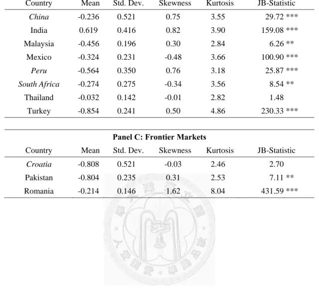
Table 7

Summary statistics of logarithms of search volume

This table presents the descriptive statistics of logarithms of search volume of each index.

Jarque–Bera statistic (JB-Statistic) is used to test the hypothesis that the data are from a normal distribution. For the name of countries in italic type mean that the data is at weekly frequency, ex: Austria. A star, double star and triple star denote significance at 10%, 5% and 1% level, respectively. Panel A, B and C provide the summary statistics of developed, emerging and frontier markets respectively.

Austria -1.435 0.400 1.39 6.88 170.89 ***

Belgium 0.128 0.223 0.11 2.68 2.56

Canada 0.522 0.279 1.72 8.22 2705.67 ***

France 0.896 0.408 1.41 6.90 1274.64 ***

Germany 0.508 0.364 1.84 9.02 3256.09 ***

Hong Kong 0.371 0.156 0.16 2.92 3.62

Italy -0.719 0.273 0.65 3.82 21.90 ***

Japan 0.555 0.381 -0.73 2.86 138.06 ***

Netherlands 0.541 0.374 1.85 8.76 2580.74 ***

Singapore 0.623 0.179 0.09 3.46 7.84 **

Spain 0.179 0.225 0.27 4.18 96.43 ***

Sweden -0.772 0.227 1.57 9.31 275.42 ***

Switzerland -0.574 0.371 1.47 6.18 176.06 ***

United Kingdom 0.054 0.311 2.19 11.01 5413.15 ***

USA-S&P 500 -0.162 0.246 1.77 13.63 8110.50 ***

USA-NASDAQ -0.472 0.306 0.84 5.64 734.06 ***

USA-DJIA 0.247 0.454 1.38 5.92 1216.91 ***

(31)

25

Table 7-Continued Panel B: Emerging Markets

China -0.236 0.521 0.75 3.55 29.72 ***

India 0.619 0.416 0.82 3.90 159.08 ***

Malaysia -0.456 0.196 0.30 2.84 6.26 **

Mexico -0.324 0.231 -0.48 3.66 100.90 ***

Peru -0.564 0.350 0.76 3.18 25.87 ***

South Africa -0.274 0.275 -0.34 3.56 8.54 **

Thailand -0.032 0.142 -0.01 2.82 1.48 Turkey -0.854 0.241 0.50 4.86 230.33 ***

Croatia -0.808 0.521 -0.03 2.46 2.70

Pakistan -0.804 0.235 0.31 2.53 7.11 **

Romania -0.214 0.146 1.62 8.04 431.59 ***

(32)

26

Figure 1:

Realized volatility and search activity

This Figure displays daily realized volatility (gray) and search volume (black) of the stock indices DJIA (USA), CAC 40 (France), SENSEX (India) and BET (Romania). The sample periods start from 2005/1/3/, 2007/1/2, 2007/10/1 and 2011/1/10 respectively and all end on 2012/2/28.

BET (Romania) where the sample periods start from 2005/1/3/, 2007/1/2, 2007/10/1 and 2011/1/10 respectively and all end on 2012/2/28. We choose 2 indices from developed markets and each from emerging and frontier markets. This can be seen from Figure 1 that realized volatility of stock index and search volume measuring local attention of index exhibit a strong co-movement over time. The correlation coefficients are 0.78, 0.69, 0.61 and 0.58 respectively.

.00 .01 .02 .03 .04 .05 .06

0 5 10 15 20 25 30

250 500 750 1000 1250

.00 .01 .02 .03 .04 .05 .06 .07 .08

0 4 8 12 16 20 24 28 32

250 500 750 1000 1250 1500 1750

.00 .01 .02 .03 .04 .05 .06 .07 .08

0 4 8 12 16 20 24 28 32

250 500 750 1000

.00 .01 .02 .03 .04 .05 .06 .07 .08

0.4 0.6 0.8 1.0 1.2 1.4 1.6 1.8 2.0

50 100 150 200 250

DJIA (USA)

SENSEX (India)

CAC 40 (France)

BET (Romania)

Realized volatility Search volume Realized volatility Search volume

(33)

27

3. Methods

3.1 Vector autoregressive model (VAR model)

In this section, we estimate a VAR model for every stock index to capture the dynamic relationship between Google search volume and stock index volatility. We study the dynamics of realized volatility and search volume by three ways: (1) Granger causality tests to examine if past volatility can significantly influence present search volume (Granger (1969) and Sims (1972)). (2) Impulse response function to see how volatility reacts over time to shock of search volume and vice versa. (3) Long-run variance decomposition to test how much of volatility can be explained by internet search volume.

First, we need to estimate a VAR(p) model:

-RV_t ∑ _, -RV_t-j ∑ _, -SV_t-j _, , (5)

-SV_t ∑ _, -RV_t-j ∑ _, -SV_t-j _, , (6)

where we decide the lag order (p) by Schwarz Criterion (SC), or named Bayes Information Criterion (BIC). The model with the lower value of SC is the one to be preferred to use.

The degree of freedom (df) used by Granger causality presented in Table 8 is just the optimal lag order (p) used for VAR model. The VAR model contains the first through sixth lags (t-1~t-6) of all the endogenous variables as p is 6. We could find that p is between 1 and 6 for daily data while weekly data have much smaller p, from 1 to 3. It makes sense that if t is this Friday and t-6 is last Thursday, then it means this week and last week when we transform to weekly frequency. At this time, p is 1. So it is normal that lag order is smaller for weekly data, where Peru has largest p=3.

And then, we examine the following 3 tests under the optimal VAR model for every index.

(34)

28

3.1.1 Granger causality test

Granger causality test, approached by Granger (1969) is to see how much of the current y can be explained by past values of y and then to examine whether adding lagged values of x can improve the explanation. If the coefficients of lagged x are statistically significant, y is said to be Granger-caused by x. That is, if search volume has statistically significant information about future volatility by t-tests or F-tests then search volume is said to Granger cause stock market volatility. Note that the statement

“x Granger cause y “does not imply that y is the effect or the result of x.

Here we use pairwise Granger causality tests to test whether an endogenous variable can be treated as exogenous in the VAR model. The null hypotheses are

“log-RV doesn't Granger cause log-SV” and “log-RV doesn't Granger cause log-SV” to see whether realized volatility is useful in forecasting search volume and whether search volume is useful in forecasting volatility at the same time. If Chi-squared (Wald) statistic is larger than critical value, such that p-value is under 0.1 with 90%

confidence level, then we can reject the null hypothesis.

3.1.2 Impulse response function (IRF)

Generally, impulse response refers to the reaction of any dynamic system in response to some external change. It traces the effect of a shock to one of the innovations on current and future values of the endogenous variables. Here we used to explore how volatility reacts over time to the shock of search volume, and vice versa.

To trace the response function, we set the number of period as 100 and use the Cholesky decomposition with the ordering, log-RV log-SV, due to the economically meaningful restriction of volatility being contemporaneously exogenous, i.e. volatility can affect search volume immediately, but search volume cannot contemporaneously affect volatility. This ordering intuitively indicates that abnormal volatility attracts