行政院國家科學委員會專題研究計畫 成果報告
深開挖破壞機制與沉陷影響範圍之研究(3/3)
計畫類別: 個別型計畫
計畫編號: NSC94-2211-E-011-001-
執行期間: 94 年 08 月 01 日至 95 年 10 月 31 日 執行單位: 國立臺灣科技大學營建工程系
計畫主持人: 歐章煜 共同主持人: 謝百鉤
報告類型: 完整報告
報告附件: 出席國際會議研究心得報告及發表論文 處理方式: 本計畫可公開查詢
中 華 民 國 95 年 11 月 2 日
深開挖破壞機制與沈陷影響範圍之研究
ABSTRACT
The excavation depth normally is the only parameter used in empirical formulas, as established by the authors and many other investigators, for predicting the ground settlement induced by excavation. The settlement influence zone predicted from such an empirical method often contradicts the field observation. For this reason, a series of parametric studies using the finite element method to fumble for the influence factors affecting the settlement influence zone induced by excavation are carried out.
The finite element method, used in this study, considers the high stiffness of the soil at small strain and is verified through the well-documented case histories. It is found that in addition to the excavation depth, the depth of the soft soil bottom, depth to the hard soil layer and the excavation width are also related to the settlement influence zone.
Furthermore, the potential failure surface, as deduced from the failure mechanism, covering the above-mentioned parameters, is used to determine the primary settlement influence zone. A method, revised from the previous work by the authors, based on the parametric study results, to predict the settlement influence zone is then proposed in this study. The nine case histories, used in the authors’ previous study, are used to verify the proposed method. Obviously, the revised method can predict the settlement profiles for all excavation stages while the other empirical methods can not. Besides, the revised method certainly can improve the accuracy in the prediction of ground settlement.
INTRODUCTION
Excavation will inevitably induce ground settlement. The profile of ground settlement should be predicted prior to excavation in order to evaluate the safety of buildings in the vicinity of excavations. The finite element method and the simplified method are two commonly used tools to predict the settlement. The former not only can predict the ground settlement but wall deflection. It also enables the engineers to understand the mechanism of settlement due to excavation and helps to design auxiliary methods to reduce the ground settlement. However, based on the authors’
experience, the finite element method usually gives a good prediction on wall deflection rather than ground settlement unless small strain theories are taken into account. On the other hand, elastoplastic theories, with the implementation of small strain theories, are usually very complicated and most of the input parameters in these models are obtained from quite complicated test procedures rather than conventional soil tests.
The simplified method is mainly derived from field observations of case histories, which many investigators (e.g., Liu et al., 2005; Finno and Bryson, 2002 ) have
delved into. This method is sometimes called as the empirical method. Since each excavation case is equivalent to a large-scale field test, it should cover all factors that may affect ground settlement. The method derived from field observations usually give a reasonable prediction on ground settlement, without much complexity, for similar excavation projects, in terms of soil conditions, construction methods, and designs.
There are some simplified methods in literature available to predict the ground settlement or wall deflection caused by excavation. However, most of them are not able to yield a very good prediction because the mechanism of induced settlement is not involved in the derivation. Some of the simplified methods represent the
envelopes of the settlement induced by all excavation stages and some of them result
in a prediction far from the truth.
The authors (Hsieh and Ou, 1998) made some progress in predicting the ground movement by classifying the settlement profile as the concave and spandrel types and established a relatively reasonable formula to predict the ground movement on the basis of field observations. The method was verified through nine case histories.
However, there are deviations between observed and computed results. The method certainly needs improvement.
From the field observations, we find that most of the existing methods only suitable to the final stages, not for all stages. The method established by the authors (Hsieh and Ou, 1998) also has a similar problem. The method certainly needs improvement to meet the actual condition. In this study, the finite element method, capable of accurately predicting the wall deflections and ground movements, is used as a tool to explore the dominant factors affecting ground movement. Then, the settlement influence zone, deduced from the mechanism of stability, is proposed.
BACKGROUND
Though many simplified methods or empirical methods for predicting ground settlement induced by excavation have been proposed, only three of them, i.e., Peck’s method (1969), Bowles’ method (1989), Clough and O’Rourke’s method (1990), are used for comparison in this study as in the previous study (Hsieh and Ou, 1998) because these methods are frequently applied in engineering practice. For saving the space, we are not going to the details of introducing the methods above and interested readers can refer to the related references.
Most of the existing methods use relatively simple parameters to predict the ground settlement. For example, Peck (1969) and Clough and O’Rourke (1990) adopted the excavation depth as the only parameter to predict the ground movement.
Bowles (1989) used the area covered by lateral wall movement as a parameter to
predict the ground movement. The authors (Hsieh and Ou, 1998) found that the settlement profile induced by excavation can be classified as the concave and spandrel types. Based on the regression analysis of field observations, we have established a method for predicting both types of settlement. In this method, the excavation depth is also the only parameter involved in the prediction of ground settlement. Based on the observed settlement profiles of the nine excavation case histories at the final stage, Hsieh and Ou’s method (1998) is of better accurate prediction than the other methods.
The key step for the prediction work is to define the settlement influence zone.
Peck (1969) proposed that the influence zone of settlement should be two or three times of the excavation depth. Clough and O’Rourke (1990) proposed that excavation in sandy soils may induce an influence zone of settlement about twice the excavation depth. As for stiff to very stiff clay, three times the excavation depth. Soft or medium soft clay, twice the excavation depth.
As discussed earlier, the types of settlement induced by excavation include the spandrel type and the concave type. The authors (Hsieh and Ou, 1998) has proposed the conception of the primary influence zone (PIZ) and the secondary influence zone (SIZ) on the basis of the principles of mechanics and regression analysis of excavation case histories. According to our study, the influence zone may extend very far and the distribution of the settlement curve includes the primary influence zone and the secondary influence zone no matter whether the settlement belongs to the spandrel type or the concave type. The curve is steeper in the primary influence zone where buildings receive more influence. In the secondary influence zone the slope of the curve is gentler and its influence on buildings is less. The primary settlement influence zone is about equal to two times excavation depth and the secondary influence zone is approximately as large as the primary influence zone.
In addition to the above, there are various other suggested values of the influence zone (Nicholson, 1987, for example).
The literature reveals that the above-mentioned methods are appropriate for the
prediction of settlement at the final excavation stage of excavation. Whether they are suitable for the stages other than the final stage remains to be resolved. Take the ground settlement of the Taipei National Enterprise Center (abbreviated as TNEC) excavation (Ou et al., 1998), as shown in Figure 1, as an example to illustrate the characteristics of settlement influence zones.
(1) As soon as excavation was started, settlement began occurring and its influence zone was large. The influence zone, for settlement, reached as far as 50 m away from the wall while the excavation depth at the third stage was 4.9 m. At this stage, no distinction between the primary influence zone and the secondary influence zone was discerned.
(2) At the fifth stage of excavation (excavation depth= 8.6 m), the primary influence zone, which was about as far as 32 m away from the retaining wall, began to be distinguishable from the settlement profile.
(3) After the fifth stage, though the excavation depth kept growing, the range of the primary influence zone was not enlarged accordingly.
From Figure 1 and the above explanation, the existing methods are not necessarily valid for every stage of excavation. The settlement influence zone certainly needs more investigation.
FINITE ELEMENT ANALYSIS
The finite element method is capable of computing the displacement at every node of a mesh after excavation, thus obtaining the deformation of the retaining wall and ground settlement as well as the stresses in an element. Though the finite element method can accurately predict the deformation and bending moment of a retaining wall, it is not capable of accurately predicting the ground settlement using the common elastoplastic models, as shown in Figure 2. The difficulty in predicting ground settlement in a braced excavation is mainly due to the fact that the soil models
are not able to simulate the deformation behavior of the soil, especially at small strain condition. In general, the better the soil model capable of simulating the deformation characteristics of soil, the higher the analysis accuracy. A number of studies were conducted to improve the accuracy of FEM predictions (e.g., Hashash and Whittle, 1996; Hight and Higgin, 1995; Stallebrass and Taylor, 1997; Finno and Calvello, 2005;
Hashash, et al., 2006). Some advance models, most of them based on the elastoplastic theory, are thus developed. However, such models are usually quite complicated and require parameters that are not necessarily obtainable through conventional soil tests.
The hyperbolic model, as proposed by Duncan and Chang (1970), has been used in the analyses of geotechnical problems quite extensively, possibly due to the fact that this type of soil model is relatively simple, conceptually understandable and easy for determining soil parameters. However, the original hyperbolic model takes the tangential Young’s modulus to simulate the primary loading and unloading-reloading modulus to model the state of elasticity. Differentiating between the primary loading sate and elastic loading state is based on the current stress level and the previous maximum stress level. The method works for most of the geotechnical problems, especially for loading problems such as dam construction, rather than unloading problems such as deep excavation. Use of the simple stress level criterion in excavation problems will cause the soil in front of the wall to be in the state of primary loading. For this reason, Hsieh and Ou (1997) introduced the concept of plasticity theory to modify the hyperbolic model where yield functions for soft clay, as derived based on Lo’s equation (Lo, 1965) and isotropic hardening rule, were used to differentiate Young’s modulus between the primary and unloading-reloading states.
The thus obtained model is relatively rational, compared with the original hyperbolic model and relatively simple, compared with the theory of plasticity.
According to the test results, clay usually possesses the high initial stiffness at small strain, about %. Unable to take this factor into consideration in the soil model will cause the prediction far from the field observation. Besides, clay also
10−3
exhibits degradation behavior where the elastic modulus or unloading-reloading modulus degrades with the increase of the stress level (Santagata et al., 1999).
Therefore, in this study the elastic Young’s modulus ( ) is assumed to be equal to the initial Young’s modulus at small strain ( ), i.e., the strain less than or equal to
%. When the strain is greater than %, the degradation of the elastic Young’s modulus can be properly simulated and expressed as a hyperbola (Hsieh et al., 2003, 2005):
E
eE
i10−3 10−3
b a SL
SL s
E s E
u i u
e
+
−
=
(1)where =undrained shear strength of the clay; and are parameters and can be obtained from the soil tests (Hsieh et al., 2003, 2005).
s
ua b
The tangential Young’s modulus ( ) from the hyperbolic model can then be rewritten as:
E
t)2
1
(
R SL E
E
t = e − f (2)where
SL
= stress level,R
f=failure ratio.For verification, a well documented and high quality deep excavation case history, the TNEC excavation, is studied. Figure 3 displays the comparison between the observed wall deflection and ground settlement and computed ones using the modified hyperbolic model with the consideration of the stiffness at small strain and the stiffness degradation phenomenon. The above mentioned model obviously can accurately predict both wall deflection and ground settlement. Therefore, the finite element method with the above model will be used for the parametric study to investigate the major factors affecting the settlement influence zone.
PARAMETRIC STUDY
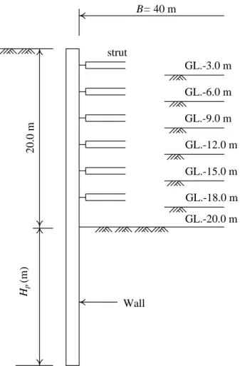
The basic excavation profile used for the parametric study is shown in Figure 4.
The soil is assumed to be homogeneous clay and has the same properties as those at the TNEC excavation site. This is because the clay at the TNEC excavation site has a complete triaxial test results at small strain, and the soil parameters used in the parametric study will adopt those at the TNEC excavation site, such as normalized initial tangent modulus ( , anisotropic strength ratio ( ) and constants a, b.
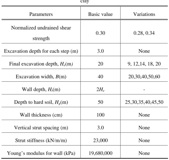
Table 1 lists the values of the key parameters of the soil and retaining-support system and their variations in the parametric study.
) / uc
i
s
E K
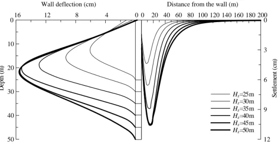
sThe typical computed wall deflections and ground settlement profiles are given in Figure 5, in which the final excavation depth,
H e
=20 m ands u
/σ v
′= 0.3, but the depth to hard soil layer, , varies from 25 m to 50 m. Casagrande’s method (1936), used to determine the pre-consolidation pressure from the result of oedometer test results, is adopted to differentiate the primary influence zone and the secondary influence zone from the settlement profile, as shown in Figure 6.H g
According to the parametric study results, it is found that the wall penetration depth ( ) has little influence on the PIZ. Woo and Moh (1990) investigated the behavior of excavations in soft clay and found that the wall depth ( ) is about to equal to 1.6 to 2.2 times final excavation depth ( ) for most of excavation case histories. Therefore, this study adopts =2.0 in the following parametric study.
H
pH
pH
eH
pH
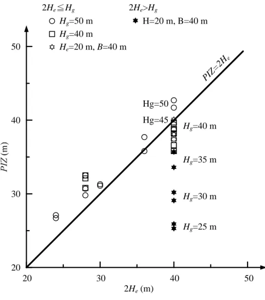
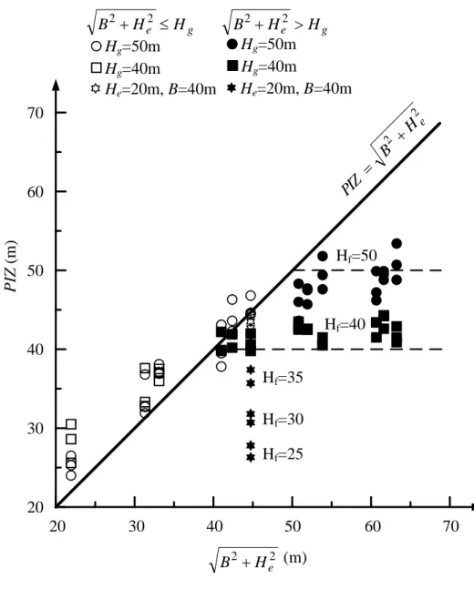
eAssuming the hard soil is very deep, about 50 meters below the ground surface, and not able to restrain the development of the failure surface, the relationship between PIZ, B, and
H
e is given in Figure 7. This figure reveals that when2 2
H e
B
+ is equal to or smaller than 2H
e, the PIZ is equal to 2H
e and otherwise,the PIZ is equal to
B
2 +H
e2 . Under the condition ofB 2
+H e 2
≤2 , it is a narrow excavation, in which the push-in failure mode is easier to happen than the basal heave failure mode or settlement influence zone due to basal heave should be smaller than that due to push-in because the failure surface engendered by basal heave is restricted by the embedded part of the wall and not able to pass through it (Figure 13b). Similarly, under the condition ofH
e2 2
H
eB
+ > 2 , it is a wide excavation, in which the basal heave mode is easier to happen than the push-in failure mode because the bearing capacity factor related to the factor of safety against basal heave decreases with the increase of excavation width (Bjerrum and Eide, 1956). Even though push-in also happens in addition to basal heave, the settlement influence zone due to push-in should be smaller than that due to basal heave.H
eAssuming the hard soil is of a limited depth, varying from 25 m to 50 m, the relationship between PIZ, B and the depth of the hard soil ( ) under the condition
of
H g
≤
+
2
2
H e
B
2 , i.e., narrow excavation, is displayed in Figure 8. As shown in this figure, when 2 , PIZ=2 ; when 2 , PIZ= . Figure 9 shows the relationship between PIZ, B and the depth of the hard soil ( ) under thecondition of
H
eH
e ≤H g H
eH
e>H g H g H g
2 2
H
eB
+ > 2 , i.e., wide excavation. As shown in this figure, whenH
e≤
+
2
2
H e
B
2H g
, PIZ=B
2+H
e2 ; whenB 2
+H e 2
>2H g
, PIZ=H g
.The maximum ground settlement of the spandrel type certainly occurs near the retaining wall. Earlier documents (Ou et al., 1993; Nicholson, 1987) claimed the maximum ground settlement of the concave type would occur at a distance of 0.5 from the wall. Nevertheless, observing the typical settlement curve of excavations, as shown in Figure 1, the location of the maximum ground settlement is determined with the starting of excavation and does not change with the increase of the excavation
H
edepth. Thus, neither Nicholson’s nor the author’s earlier study conforms to the actual conditions.
Figure 10, based on the parametric study results, displays the relationship between the location of maximum settlement and PIZ. As shown in the figure, the location of the maximum settlement of the concave type can be determined by the equation: (Note: definition of can be referred to Figure 2). As elucidated earlier, the primary influence zone (PIZ) is determined as soon as the excavation is started and the location of the maximum settlement ( ), which does not move with the continuation of excavation, is determined accordingly, too.
PIZ
D
m =0.33D
mD
mEarlier studies, based on the limited field data, suggest that the settlement at the transition point between the PIZ and SIZ is about equal to 0.1 times the maximum ground settlement, that is,
δ
i =0.1δ
vm. However, based on the parametric study, it is found from Figure 11 thatδ
i can be reasonably estimated by assumingδ i
=δ vm
/6.Based on the parametric study above, the original prediction method for the concave settlement profile is then revised as shown in Figure 12b, in which the primary influence zone (PIZ) is not necessarily equal to 2 . In addition to the excavation depth, the excavation width, depth to hard soil and depth of the soft soil bottom are also related to the PIZ.
H
eDETERMINATION OF THE PRIMARY INFLUENCE ZONE
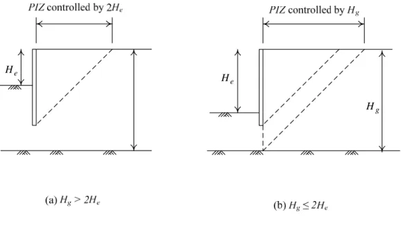
The push-in and the basal heave are two main overall failure modes of excavations. As shown in Figure 13a, the push-in is caused by the earth pressures, reaching the limiting state, on both sides of the retaining wall, which is thereby moved, a large distance, toward the excavation zone (especially the part embedded in soil) until reaching the full-zone failure. The analysis views the retaining wall as a free
body and the external forces on the wall and internal forces of the wall are in
equilibrium. The factor of safety against push-in or penetration depth of the wall can thus be obtained.
The basal heave arises from the weight of soil outside the excavation zone exceeding the bearing capacity of soil below the excavation bottom, causing the soil to move and the excavation bottom to heave so much that the whole excavation collapses. Figure 13b also shows a possible form of basal heave. When analyzing the basal heave, we should assume several possible basal heave failure surfaces and find their corresponding factors of safety according to mechanics. The surface having the smallest factor of safety is the most likely potential failure surface or critical failure surface.
According to the loading behavior of soil, strain in soil will increase greatly when soil is going to fail or has failed. The movement or strain within the primary influence zone is rather large and we can reasonably assume the primary influence zone is the potential failure zone. According to the elucidation of the mechanism of overall shear failure above, failure due to excavation can be mainly divided into push-in failure and basal heave failure. The former may happen in sand, clay, or any other type of soil (hard soils excluded) while the latter happens only in soft clay.
Since the design of the strutted wall is based on the conception of the free earth support method, not only the bottom of the retaining wall has movement but also the soil below the wall bottom may exhibit movement. If we suppose that the movement of the soil is not restricted (i.e., hard soils are very far underneath), the formation of the active failure in back of the retaining wall will not be obstructed and the active failure zone will be about twice as wide as the excavation depth (2 ). When the hard soil is shallow enough to restrict the movement of the soil, the range of the active failure zone will be about the same as the depth of the hard soil. Such observations are consistent with one of the parametric study results shown in Figure 8. Therefore, the potential failure zone based on the push-in failure mode, occurring in narrow
H
eexcavations or the condition of
B 2
+H e 2
≤2 , can be determined (Figure 14) as follows:H
e( H
eH
g)
PIZ
1= min 2 ,
(3)where
H
g = depth of the hard soil.The hard soil in this study refers to the soil which will not occur the basal heave or push-in, such as rock, gravel, etc.
Excavation in soft clay may also induce basal heave. Based on the results of the parametric study shown in Figure 9, the potential basal heave failure surface can be the one with the wall top as axis and the diagonal as radius (X in Figure 15). If the sandy or the hard soil locates shallower, the potential basal heave failure surface will then be tangential to the sandy or hard soil and the potential basal heave failure range in back of the wall will be close to the distance to the soft clay bottom from the
ground surface. Thus, the potential failure zone based on the basal heave failure mode, occurring in wide excavations or the condition of
B 2
+H e 2
>2 , can bedetermined as follows (Ou et al., 2005):
H
e(
2 2)
2 min
H
f,B H
ePIZ
= + (4)where
H
f= depth of the soft clay bottomB = excavation width
Both and are potential failure zones. The primary influence zone of excavation-induced settlement is the maximum of the potential failure zones. This observation is also consistent with the parametric study results (Figure 7). Thus, the primary influence zone is the larger of or :
PIZ
1PIZ
2PIZ
1PIZ
2) , max( PIZ
1PIZ
2PIZ =
(5) If the hard soil locates very deep and does not affect the settlement influencezone, with the occurrence of basal heave,
B
2 +H
e2 >2 , is greater than , which in turns causesH
eB
H e
73 .
1
B
2+H
e2 <1.15B. Therefore, for simplification,2 2
H
eB
+ in Eq. 4 may be replaced by excavation width, . Eq. 10 thus can be rewritten asB
( H B )
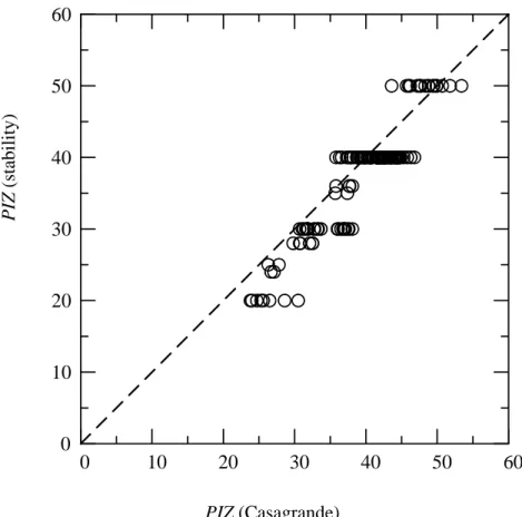
PIZ
2= min
f,
(6)The primary influence zone (PIZ) for each hypothetical case in the parametric study can therefore be determined based on Eqs 3, 6 and 5. Figure 16 reveals the relationship of the PIZ determined through the proposed method and those directly deduced from the settlement profile using Casagrande’s method. We can see from the figure that the PIZ derived from the proposed method, i.e., Eqs 3, 6 and 5, agree very well with the actual primary settlement influence zone.
DETERMINATION OF THE SPANDREL SETTLEMENT PROFILE
The above parametric study using the finite element method and subsequent derivation of the primary influence zone mainly focus on the concave settlement profile. With the spandrel settlement profile, the soil near the wall normally has a relative large movement. To reproduce such behavior using the finite element method normally requires the use of the interface element. However, the introduction of the interface element in analysis requires some extra parameters, which make the analysis more complicated. Instead, the establishment of the method for predicting the
spandrel settlement profile will use a reasonable inference and case studies, just as in the previous study.
The principle of Saint Venant (Timoshenko and Goodier, 1951) states that if some distribution of forces acting on a portion of the surface of a body is replaced by a different distribution of forces acting on the same portion of the body, then the effects of the two different distributions on the parts of the body far away from the region of application of the forces are essentially the same, provided that the two distributions
of the forces have the same resultant force. As described in the previous study, different excavation and strut installation procedures will results in different states of stresses for the soil near the wall (i.e., primary influence zone), which in turn yield different shapes of settlement profile, i.e., concave type and spandrel type. As discussed in the preceding section, the primary influence zone can be obtained from the potential failure surface, deduced from the failure mechanism of excavations. The potential failure surface or failure mechanism is mainly related to the subsurface soil properties and geometry of excavations, and has little relation to the excavation and strut installation procedures as long as the final excavation depth and strut-retaining stiffness are the same. Therefore, Eqs 3, 6 and 5 can also be used to determine the primary influence zone of the spandrel settlement profile.
Such different excavation and strut installation procedures but with the same resultant force, i.e., active force, will induce the same or close state of stresses for the soil far away from the wall and therefore the corresponding the settlement beyond the primary influence zone in the concave settlement profile and spandrel settlement profile may be the same under such conditions. This implies that the settlement beyond the primary influence zone is not affected by the shapes of settlement profile in the primary influence zone. We therefore assume that the settlement at the
transition point in the spandrel settlement profile is equal to that in the concave
settlement profile, i.e.,
δ i
=δ vm
/6. The spandrel settlement profile is then revised, as shown in Figure 12a.VERIFICATION OF THE PROPOSED METHOD
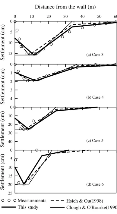
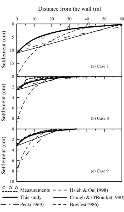
The authors in their previous study (Hsieh and Ou, 1998) adopted nine case histories to verify the proposed method. As described in that study, cases 1 to 6 have the concave type of settlement profile while cases 7 to 9 have the spandrel type of settlement profile. For proving if the new method capable of enhancing predictability,
this study adopts the same case histories. For comparison, the Hsieh and Ou’s method (1998), along with other empirical methods, are also indicated in each case history.
Since all of the excavations were described in that paper, for saving the space, this study only briefs the basic geometry of the excavations. Interested readers can refer to Hsieh and Ou (1998) for more descriptions of the excavations and subsurface
geological profiles.
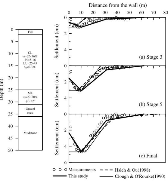
Case 1, TNEC excavation, is a 40 m wide excavation, with 35 cm deep and 90 cm thick diaphragm wall. The final excavation depth was 19.7 m. The basement was constructed using the top down construction method, which included 16 construction stages (note: 7 excavation stages). In addition to the final stage, settlement profiles at two intermediate stages, i.e., stage 5 ( =8.6 m) and stage 9 ( =15.2 m) are also used for verification.
H e H e
At stage 5, concerning the push-in failure, twice the excavation depth, , is 17.2 m, and the cobble-gravel soil is regarded as a hard soil, =46 m, =17.2 m. With the depth of the bottom of the soft clay ( ) being 37.5 m, =40 m,
= 37.5 m. Thus, we will conclude the primary influence zone ( ) is 37.5 m.
Figure 17a shows the comparison between the new method and the other two methods.
At stage 9, =30.4 m, =46 m, =30.4 m; =40 m, =37.5 m,
=37.5 m. Thus, we can conclude the primary influence zone is 37.5 m
( =37.5 m). Figure 17b shows the comparison between the new method and the other two methods. As displayed in Figures 17a and b, the settlement profile
computed from the new method satisfactorily conforms to the field measurement while those derived from the other two methods are far from the field measurements.
H
e2
H g PIZ 1
H
fB
PIZ 2 PIZ
H e
2
H g PIZ 1 B H f
PIZ 2
PIZ
At final stage, =39.4 m, =46 m, =39.4 m; =40 m, =37.5 m, =37.5 m. Thus, we can conclude the primary influence zone is 39.4 m
H e
2
H g PIZ 1 B H f
PIZ 2
( m). Figure 17c shows that the new method can enhance the prediction,
compared with the previous method. The settlement profile derived from Clough and O’ Rourke’s method can lead to a satisfactory settlement envelope as far as the primary influence zone is concerned, though the secondary influence zone is obviously ignored.
PIZ
From the above discussion, the primary influence zones at stage 5, 9 and 13 (final stage) are found to be 37.5 m, 37.5 m and 39.4 m, respectively. Obviously, the
primary settlement influence zones remain unchanged or change little with the
increasing excavation depth, which conforms the field observation as shown in Figure 1.
Case 2 is an excavation with 60 m long and 35 m wide. The diaphragm wall was 31m in depth and 80 cm in thickness. The final excavation depth was 18.45 m. The braced excavation method was adopted with 7 excavation stages. In addition to the final stage ( =18.45 m), settlement profiles at two intermediate stages, i.e., stage 3 ( =6.9 m) and stage 5 ( =13.2 m) are also used for verification.
H e
H e H e
At stage 3, according to the excavation geometry and the soil profile displayed in Figure 18, we have the following data: =13.8 m, =31 m, =13.8 m;
=35 m, =31 m, =31 m. Thus, we can conclude the primary influence zone is 31 m (
H e
2
H g PIZ 1
B H f PIZ 2
= 31
PIZ
m). At stage 5, =26.4 m, =31 m, =26.4 m;=35 m, =31 m, =31 m. Thus, we can conclude the primary influence zone is 31 m (
H e
2
H g PIZ 1
B H f PIZ 2
= 31
PIZ
m). Figures 18a and b shows the comparisons between the measured settlement profiles and those computed separately from the three methods for stages 3 and 5, respectively. As shown in these figures, the settlement profiles derived from the new method are close to the field measurements. On the other hand, the results computed using Clough and O’Rourke’s method and Hsieh and Ou (1998)are far from the field measurements.
At final stage, =36.9 m, =31 m, =31 m; =35 m, =31 m,
=31 m. Thus, we can conclude the primary influence zone ( ) is 31 m.
Figure 18c shows that the settlement computed from the new method has a better prediction accuracy than the other two methods. Obviously, the primary settlement influence zones estimated from the new method, all equal to 31 m, does not change with the increasing excavation depth, which conforms the field observation as shown in Figure 1
H e
2
H g PIZ 1 B H f
PIZ 2 PIZ
Case 3 is a Tokyo subway excavation with the 30 m excavation width. The final excavation depth was 17 m. According to the geological condition described in Hsieh and Ou (1998), if the dense sand, locating at a depth of 37 m below the ground surface, is treated as hard layer, then we have the following data: =34 m,
=37 m, =34 m; =30 m, =37 m, =30 m. Thus, we can conclude the primary influence zone ( ) is 34 m. Following Figure 12, Figure 19a shows the new method is of better accurate prediction than Hsieh and Ou (1998). Again, Clough and O’Rourke’s method is unable to predict the settlement profile, even unable to envelope the settlement profile.
H e
2
H g PIZ 1 B H f PIZ 2
PIZ
Case 4 is a 50 m wide excavation. The final excavation depth was 18.5 m.
According to Hsieh and Ou (1998), if the hard rock, locating at a depth of 44 m below the ground surface, is treated as hard layer while the London clay, between 10 m and 30 m, is regarded as the stiff soil, which would not engender the basal heave. Then, we have the following data: =37 m, =44 m, =37 m; =50 m,
=0m, =0 m; =37 m. Figure 19b shows that both the new method and Hsieh and Ou’s method can result in good prediction while Clough and O’Rourke’s method provides good envelope of the settlement profile for the soil near the wall but neglects the settlement in the secondary zone.
H e
2
H g PIZ 1 B
H f PIZ 2 PIZ
Case 5 is the Chicago subway excavation with the 12.2 m excavation width. The final excavation depth was 12.2 m. According to Hsieh and Ou (1998), if the hard rock, locating at a depth of 25 m below the ground surface, is treated as hard layer while the clay, between 5 m and 16.2 m, is regarded as the soft soil. Then, we have the following data: =24.4 m, =25 m, =24.4 m; =12.2 m, =16.2 m,
=12.2 m; =24.4 m. Figure 19c shows that both the new method and Hsieh and Ou’s method can result in good prediction while Clough and O’Rourke’s method provides good envelope of the settlement profile.
H e
2
H g PIZ 1 B H f
PIZ 2 PIZ
Case 6 is the Oslo subway excavation, with the 11 m excavation width. The final excavation depth was 11m. According to Hsieh and Ou (1998), if the bedrock,
locating at a depth of 16 m below the ground surface, is treated as a hard layer while the clay, between 2 m and 16 m, is regarded as a soft soil. Then, we have the
following data: =22 m, =16 m, =16 m; =11 m, =16 m,
=11 m; =16 m. Figure 19d shows that the new method is of better accuracy in prediction ground settlement than the methods of Hsieh and Ou (1998) and Clough and O’Rourke (1990).
H e
2
H g PIZ 1 B H f
PIZ 2 PIZ
Case 7 is the Far-East Enterprise Center excavation, located in Taipei, with the 64 m excavation width. The final excavation depth was 20 m. According to Hsieh and Ou (1998), if the gravel soil, at a depth of 32 m below the ground surface, is treated as a hard layer. The clay, between 8 m and 32 m, is regarded as a soft clay. Then, we have the following data: =40 m, =32 m, =32 m; =64 m, =32 m,
=32 m; =32 m. Figure 20a displays that both the new method and Hsieh and Ou’s method can result in very good prediction in ground settlement while the other three methods, Bowles (1986), Clough and O’Rourke (1990) and Peck (1969), are not able to have a good prediction.
H e
2
H g PIZ 1 B H f
PIZ 2 PIZ
Case 8 is the Bell Common Tunnel in England, with the 40 m excavation depth and 9 m excavation depth. According to Hsieh and Ou (1998), if the gravel soil, at a depth of 30 m below the ground surface, is treated as a hard layer. The clays, above 30 m below the ground surface, all have relative high undrained shear strength and are therefore treated as a stiff soil, which would not induce basal heave. Then, we have the following data: =18 m, =32 m, =18 m; =40 m, =0 m,
=0 m; =18 m. Figure 20b displays that both the new method and Hsieh and Ou’s method result in very good prediction in ground settlement while the other three methods, Bowles (1986), Clough and O’Rourke (1990) and Peck (1969), are not able to have a good prediction.
H e
2
H g PIZ 1 B H f
PIZ 2 PIZ
Case 9 is the Neasden Underpass in north London, with the 8.5 m final
excavation depth and 20 m excavation width. According to Hsieh and Ou (1998), if the hard rock, at a depth of 30 m below the ground surface, is treated as a hard layer.
The clays, above 30 m below the ground surface, all have relative high undrained shear strength and are all treated as a stiff soil, which would not cause basal heave.
Then, we have the following data: =17 m, =30 m, =17 m; =20 m,
=0 m, =0 m; =17 m. Figure 20c displays that both the new method and Hsieh and Ou’s method yield very good prediction in ground settlement while the other three methods, Bowles (1986), Clough and O’Rourke (1990) and Peck (1969), are not able to have a good prediction.
H e
2
H g PIZ 1 B
H f PIZ 2 PIZ
As demonstrated in the studies of cases 1 to 9 (Figures 17 to 20), we can find that the new method can have a substantial improvement in the prediction of settlement at the intermediate stages while has some improvements for the settlement at the final stage, compared with the authors’ previous work (Hsieh and Ou, 1998). This is because the values of , used in the authors’ previous work, are not deviated too much from the values of other parameters like
H e
2
B , H g
andH f
. As for theintermediate stages, values of 2
H e
are usually much smaller than the parameters (B ,
and ), and one of those parameters is often the controlling parameters to determine the primary settlement influence zone.H g H f
CONCLUSION
The authors developed a method to predict the ground settlement in their previous work, suitable for the concave as well as the spandrel settlement profiles. The method was verified through the nine case histories, by which the settlements computed from the method were close to the field measurements. However, the previous method used the excavation depth as the only parameter to determine the settlement influence zone like the other empirical methods, e.g., Clough and O’Rourke (1990), Peck (1969) and Bowles (1986) and so on. This causes the primary settlement influence zone
increasing with the excavation depth, which contradicts the field observation, i.e., the settlement influence zone remains unchanged or changes little, with the increasing excavation depth. Therefore, a new method, with the determination of the primary influence zone, location of the maximum settlement and settlement at the transition point between the primary influence zone and settlement influence zone, is proposed, based on the parametric study results using the finite element method and failure mechanism. The new method is obviously able to predict the settlement profile for all excavation stages while the previous method and most of the empirical methods can not. Besides, the following conclusions can be drawn:
1. Since the primary settlement influence zone is defined as the one with relatively large settlement or angular distortion, according to the stress-strain behavior of soil, we can reasonably assume the primary influence zone is the potential failure zone, in which the soil is subjected to relatively large strain or movement. From the parametric study results, it is found that in addition to the excavation depth, the excavation width, the locations of hard soil layer and bottom of soft clay are also related to the primary influence zone, which forms a basis of the new method. The
proposed new method certainly have a substantial improvement in predicting the ground settlement for excavations with twice the excavation depth very different from the other parameters, such as excavation width, depth to hard soil layer and depth of bottom of soft clay.
2. Although there are two basic types of settlement profile, concave and spandrel, induced by excavation, the settlement influence zone is basically nothing to do with types of settlement profile. Besides, the settlement at the transition point between the primary influence zone and secondary influence are basically the same.
Such derivation causes the proposed new method to be quite consistent among the two settlement profiles.
3. Based on the field observation, the location of the maximum ground settlement usually remains constant, i.e., does not change with the excavation depth. Such phenomenon is also verified through the finite element method. Based on the results from the parametric study, we have found the location of maximum ground settlement,
D m
=PIZ/3.
References
Bjerrum, L. and Eide, O. (1956), Stability of strutted excavation in clay, Geotechnique, Vol. 6, pp. 32-47.
Bowles, J. E. (1986), Foundation Analysis and Design, 4th Ed., McGraw-Hill Book Company, New York, U.S.A.
Casagrande, A. (1936), The determination of the Pre-Consolidation Load and Its Practical Significance, Discussion D-34, Proceedings of the First International Conference on Soil Mechanics and Foundation Engineering, Cambridge, Vol. III, pp.60-64.
Clough, G. W. and O'Rourke, T. D. (1990), Construction-induced movements of in situ walls, Design and Performance of Earth Retaining Structures, ASCE Special Publication, No. 25, pp.439-470.
Duncan, J.M. and Chang, C.Y. (1970), Nonlinear analysis of stress and strain in soils, Journal of the Soil Mechanics and Foundations Division, ASCE, Vol. 96, No. 5, pp. 637-659.
Finno, R. J. and Bryson, L. S. (2002), Response of building adjacent to stiff excavation support system in soft clay, Journal of Performance of Constructed Facilities, ASCE, Vol. 16, No. 1, pp. 10–20.
Finno, R. J. and Calvello, M. (2005), Supported excavations: observational method and inverse modeling, Journal of Geotechnical and Geoenvironmental Engineering, ASCE, Vol. 131, No. 7, pp. 826–836.
Hashash, Y. M. A., Marulanda, C. M., Ghaboussi, J. and Jung, S. (2006), Novel approach to integration of numerical modeling and field observations for deep excavations, Journal of Geotechnical and Geoenvironmental Engineering, ASCE, Vol. 132, No. 8, pp. 1019–1031.
Hashash, Y. M. A. and Whittle, A. J. (1996), Ground movement prediction for deep excavations in soft clay. Journal of Geotechnical Engineering, ASCE, Vol. 122, No. 6, pp. 474–486.
Hight, D.W. and Higgins, K.G. (1995), An approach to the prediction of ground movements in engineering practice: background and application, Int. Symp. on Pre-failure Deformation Characteristics of Geomaterials, IS-Hokkaido, Sapporo, pp. 909-945.
Hsieh, P. G., Kung, T. C., Ou, C. Y., and Tang, Y. G. (2003), Deep excavation analysis with consideration of small strain modulus and its degradation behavior of clay, Proceedings 12th Asian Regional Conference on Soil Mechanics and Geotechnical Engineering, pp. 785-733.
Hsieh, P. S., Kung, T. C., and Ou, C. Y. (2005), Simulation of stress-strain curve under undrained condition, Geotechnical Engineering, SEAGS, No. 1, Vol. 36, pp.
91-95.
Hsieh, P. G. and Ou, C.Y. (1997), Use of the modified hyperbolic model in excavation analysis under undrained condition, Geotechnical Engineering Journal, SEAGS, Vol. 28, No. 2, pp. 123-150.
Hsieh, P.G. and Ou, C.Y. (1998), Shape of ground surface settlement profiles caused by excavation, Canadian Geotechnical Journal, Vol. 35, No. 6, pp. 1004-1017.
Liu, G. B., Ng, C. W. W., and Wang, Z. W. (2005), Observed performance of a deep multistrutted excavation in Shanghai soft clays, Journal of Geotechnical and Geoenvironmental Engineering, ASCE, Vol. 131, No. 8, pp. 1004–1013.
Lo, K. Y. (1965), Stability of slopes in anisotropic soils, Journal of the Soil Mechanics and Foundations Division, ASCE, Vol. 91, No. 4, pp. 85-106.
Nicholson, D. P. (1987), The design and performance of the retaining wall at Newton station, Proceeding of Singapore Mass Rapid Transit Conference, Singapore, pp.
147-154.
Ou, C.Y., Heish, P. G. and Chiou, D. C. (1993), Characteristics of ground surface settlement during excavation, Canadian Geotechnical Journal, Vol. 30, pp.
758-767.
Ou, C. Y., Hsieh, P. G. and Duan, S. M. (2005), A Simplified Method to Estimate the Ground Surface Settlement Induced by Deep Excavation, Geotechnical Research Report No. GT200502, Department of Construction Engineering, National Taiwan University of Science and Technology.
Ou, C.Y., Liao, J. T. and Lin, H. D. (1998), Performance of diaphragm wall constructed using top-down method, Journal of Geotechnical and Geoenvironmental Engineering, ASCE, Vol. 124, No. 9, pp. 798-808.
Peck, R. B. (1969), Deep excavation and tunneling in soft ground, Proceedings of the 7th International Conference on soil Mechanics and Foundation Engineering, Mexico City, State-of-the-Art Volume, pp. 225-290.
Santagata, M.C., Germaine, J.T. and Ladd, C.C. (1999) Initial stiffness of K0-normally consolidated Boston Blue Clay measured in the triaxial apparatus, Pre-failure Deformation Characteristics of Geomaterials, Balkema, Rotterdam.
Stallebrass, S.E. and Taylor, R.N. (1997), The development and evaluation of a constitutive model for the prediction of ground movements in overconsolidation clay, Geotechnique, Vol. 47, No. 2, pp. 235-253.
Timonshenko, S. and Goodier, J. N. (1951), Theory of Elasticity, 2nd edition, McGraw-Hill Book, Co., New York.
Woo, S. M. and Moh, Z. C. (1990), Geotechnical characteristics of soils in Taipei basin, Proceeding of 10th Southeast Asian Geotechnical Conference, Special Taiwan Session, Taipei, Vol. 2, pp. 51-65.
Table 1: Basic conditions and variations for parametric study of excavations in soft clay
Parameters Basic value Variations
Normalized undrained shear strength
0.30 0.28, 0.34
Excavation depth for each step (m) 3.0 None Final excavation depth, He(m) 20 9, 12,14, 18, 20
Excavation width, B(m) 40 20,30,40,50,60
Wall depth, Ht(m) 2He -
Depth to hard soil, Hg(m) 50 25,30,35,40,45,50
Wall thickness (cm) 100 None
Vertical strut spacing (m) 3.0 None
Strut stiffness (kN/m/m) 23,000 None
Young’s modulus for wall (kPa) 19,680,000 None
D m
GL.-6.0 m GL.-3.0 m
GL.-9.0 m GL.-12.0 m GL.-15.0 m GL.-18.0 m GL.-20.0 m B= 40 m
2 0 .0 m H
p(m)
strut
Wall
FIGURE 4 Typical excavation profile used in the parametric study
50 40 30 20 10 0
De p th (m )
16 12 8 4 0
Wall deflection (cm)
0 20 40 60 80 100 120 140 160 180 200
12 9 6 3 0
S ettl em en t (c m )
H
g=25 m H
g=30 m H
g=35 m H
g=40 m H
g=45 m H
g=50 m Distance from the wall (m)
FIGURE 5 Variation of the typical computed wall deflection and ground settlement profiles with the depth to the hard soil layer
δ
iδ
vmPIZ
=2 H
ePIZ (m)
H
e2
2 2
H
eB PIZ = +
e
e
H
H B
2+
2≤ 2
e
e
H
H
B
2+
2> 2
H
g=25 mH
g=30 mH
g=35 m Hg=45H
g=40 m Hg=50PIZ=2H
e
2He≦Hg
H
g=50 mH
g=40 mH
e=20 m, B=40 m2He>Hg
H=20 m, B=40 m
2He(m)
20 30 40 50
20 30 40 50
FIGURE 8
Relationship between the primary influence zone and the various parameters (He, Hg, B) under the condition ofB 2 + H e 2 ≤ 2 H e
Hf=35 Hf=30 Hf=25
Hf=40 Hf=50
H
g=50mH
g=40mH
g=50mH
g=40mH
e=20m, B=40mH
e=20m, B=40m20 30 40 50 60 70
20 30 40 50 60 70
PIZ (m)
FIGURE 9
Relationship between the primary influence zone and the various parameters (He, Hg, B) under the condition ofe
e H
H B 2 + 2 > 2
2 2
H e
B +
(m)2 2
H e
B PI Z
+
=
g
e H
H
B 2 + 2 ≤ B 2 + H e 2 > H g
PI Z
D . 4 0
m ax
=
PIZ D
. 23 0
ma x =
PI Z
D
. 33 0
ma x
=
ma x D (m )
vm i
δ δ
. 16
= 0
vm
i
δ δ
. 25
= 0
vm i
δ = 0 . 1 δ
δ
vm
i δ
PIZ d
vmv
δ δ
/vmv
δ δ
/PIZ d
{
H
eH
gH
e(b) H
fSand or hard soil
FIGURE 15 The primary settlement influence zone derived from the failure mode“basal heave"
Soft soil H
fB
H
e(a)
X
0 10 20 30 40 50 60 0
10 20 30 40 50 60
PIZ (Casagrande)
PI Z (stability)
FIGURE 16 Relationship between the PIZ determined through the proposed method and those directly from the settlement profile using Casagrande's method
(unit: meter)
0
0
Distance from the wall (m)
Sett lement (cm ) Sett lement (cm )
Hsieh & Ou(1998)
Clough & O'Rourke(1990) (a) Stage 3
Sett lement (cm )
Measurements This study
(b) Stage 5
(c) Final
0 10 20 30 40 50 60 70 80
4 2 0
4 2
6 4 2
Fill
CL
=26-36%
PI=8-16 LL=25-45
su=0.3 v'
ML
=22-30%
=32°
Gravel rock
Mudstone