成本導向多標籤學習演算法與應用

(1)

國立臺灣大學電機資訊學院資訊工程學研究所博士論文

Department of Computer Science and Information Engineering College of Electrical Engineering and Computer Science

National Taiwan University Doctorial Dissertation

成本導向多標籤學習演算法與應用

Cost-Sensitive Multi-Label Classification with Applications

駱宏毅 Hung-Yi Lo

指導教授：林守德博士、王新民博士

Advisors: Shou-De Lin, Ph.D. and Hsin-Min Wang, Ph.D.

中華民國 102 年 1 月

January 2013

(2)

i

(3)

ii

誌謝

「然而因著神的恩，我成了我今天這個人」哥林多前書第十五章 10 節上

讀博士班期間曾經歷過許許多多挑戰、困難和挫折。難以言喻的奇妙經歷點滴在心裡，

包括入學前教會的鄭桂忠弟兄向我介紹林守德教授、考最後一科資格考時經歷主的平安與能力、參與資料探勘比賽時從詩歌中被感動並得著信心與鼓勵、以及投第三篇期刊論文時得到許多意外的幫助。這些事都非我能力所能計劃並安排的，見證神的恩典與看顧，將一切榮耀與感謝歸給神。

我要感謝本篇論文最重要的兩位推手，我的指導教授王新民老師和林守德老師。我從民國 94 年一月即開始至中研院資訊所服國防役，役滿繼續擔任研究助理的工作。直到博士班畢業為止，這八年的時間都受王新民老師的指導與栽培。在前幾年研究不太順利的時候，非常感謝王老師對我非常有耐心、一直鼓勵我。每一次在對研究覺得失望灰心時跟老師個別面談，

都讓我重新燃起信心和鬥志。也謝謝老師讓我在研究上有自由發揮的空間，訓練我有獨立自主研究的能力。老師在開會時總是非常仔細地深入報告的細節，並提出許多寶貴的建議。此外要感謝老師非常用心且花費大量時間在我每一篇投稿的論文、報告投影片及海報上。每一次老師都是從頭到尾、每字每句仔細地看過並反覆考慮過。王老師的認真、嚴謹、仔細，以身做責示範作研究應有的態度跟用心，實在是我永遠學習的榜樣。

也非常感謝林守德老師在我進入台大讀博士班後的指導。我是林老師來到台灣大學後的第一屆博士班學生。老師始終非常平易近人，營造了非常充滿研究熱忱、團結且有向心力的實驗室氣氛。幾次我遭遇困境去找林老師，他總是在學生的角度替學生們著想並盡可能地給予幫助。在 97 年我們參加了資料探勘比賽。開始只是我對於期末作業的提議，但老師非常認真對待，帶動了實驗室對於參加比賽得獎的氣氛，最終也得到了連續多年得獎的偉大成果。

此外，老師也給我非常多的成長機會，如擔任教學助理、在國際會議發表 Tutorial、和指導實驗室裡的學弟妹作研究。這些事都對於我在知識和為人處事上的長進非常有幫助。老師對於帶領實驗進步非常有智慧，每學期對實驗室開會或研究上細節的安排都非常值得我學習。

老師對於做人、做事、和做研究「態度」上的要求，也是我永遠學習榜樣。

在博士論文計畫審查階段，感謝陳銘憲老師、林軒田老師、陳信希老師等委員們不吝指教地給予許多寶貴意見。不僅對於我的研究主題，也對於我正在投稿中的期刊論文修訂非常有幫助。博士學位考試時，林智仁老師、林軒田老師、陳銘憲老師、交通大學簡仁宗老師、

成功大學曾新穆老師、台灣科技大學李育杰老師等口試委員們精闢切要的論點與建議，幫助我能更完善地修訂論文內容。在此特別感謝我的碩士班指導教授李育杰老師。李老師是帶領我進入資料探勘與機器學習領域的入門導師。老師一點一滴教導我資料探勘的知識，為我後來在中研院和讀博士班期間的研究打下良好的基礎。在畢業後許多人生選擇的轉彎路口，老師也都給我許多寶貴的建議與幫助。謝謝您一路以來的諄諄教誨！

(4)

iii

感謝中研院語音語言與音樂處理實驗室的同事們，陪伴我完成這篇論文。謝謝王如江、

陳冠宇、李鴻欣、黃信德、簡御仁、陳傳祐、施羽芩、游廷碩、陳羿帆…等，尤其感謝如江是我研究上的好夥伴、感謝廷碩對於出國和業界工作方面跟我分享很多寶貴的經驗、鴻欣追根究底的研究精神非常令我佩服。謝謝台灣大學機器發明與社群網路探勘的同學們，特別謝謝曾與我合作過的夥伴蕭卓毅、張峻銘、江宗憲、殷圖駿、魏吟軒、游書豪、蔡青樺。也感謝李政德陪我一起走過這五年多，跟我分享很多研究與出國經驗、謝謝楊政倫幫我改論文的英文、謝謝楊明翰和何建彤教我認識鬥塔遊戲，為枯燥的研究增添不少樂趣、謝謝我的鄰座顏君釗、張博詞、林瑋詩幫我處理很多電腦或座位方面的問題、感謝嚴恩勗跟我合作過一次印象深刻的線性分類器的報告、感謝解巽評常常提供實驗室裡鮮為人知的神祕資訊、謝謝賴弘哲、曾建霖在我畢業找工作時給我很多資訊跟幫助。此外，非常感謝資工系資格考讀書會的夥伴們，感謝王界人、林育仕、吳信宏、郭人瑋、何立勇、曾志傑、陳泰瑜、董才業。沒有你們的陪伴、互相教導學習，我可能連資格考都通過不了。尤其志傑後來成為我在教會中的好同伴與配搭，非常感謝他。也感謝與我一同參與 KDD Cup 的同學和老師們，很高興能與大家一同努力過。感謝在博士班期間認識的朋友們，感謝在 ISMIR 2009 認識的楊奕軒博士是研究上很好的夥伴，也是值得學習的榜樣、謝謝胡敏君博士在我畢業和找工作的過程中給我很多幫助、謝謝任佳珉跟黎欣捷陪伴我渡過難忘的 ICASSP 2011 布拉格之旅。

最後感謝我親愛的家人們，謝謝爸爸、媽媽從小到大對我的栽培，讓我能毫無後顧之憂地攻讀博士學位。感謝我的老婆在我讀博士班期間一直無怨無悔地陪伴並支持。在許多熬夜趕工的夜晚，謝謝老婆辛苦地獨自照顧家庭跟小孩。並且感謝老婆生了兩個可愛的兒子在我研究的路上陪伴我，雖然兒子常常調皮搗蛋，但讓我的生活增添了許多純真的歡笑！最後感謝我的妹妹、岳父、岳母，及許多其他親友們的支持與照顧。謹將本篇論文獻給我最愛的你們。

駱宏毅謹誌民國 102 年一月

(5)

iv

摘要

本論文的第一部份研究一個新的機器學習問題，稱之為成本導向多標籤分類問題。在這個問題中，每一筆資料的不同標籤可以有不同的分類錯誤成本。我們首先利用機器學習演算法中簡化問題的技術，將成本導向多標籤分類簡化成成本導向單標籤分類問題。此外，我們提出了一個基於基底擴展模型的方法來解成本導向多標籤分類問題。此方法稱為一般化 k 標籤集合群體分類法。此群體分類中，每一個基底函式是一個標籤冪集合分類器。基底函式的係數的學習方式是最小化成本導向錯誤率。我們推導出快速的求解係數的計算方式。此方法也可以應用在一般的多標籤分類問題。在一般的多標籤分類問題和成本導向多標籤分類問題的實驗結果都證實我們提出的新方法的預測效果更好。

如何在應用問題中找出分類錯誤成本，是一個重要的實務問題。本論文的第二部份研究兩個成本導向分類問題的應用：醫學影像分類與社群標籤預測。在醫學影像分類問題中，我們發現了正例資料中的病患不平衡問題。這個問題嚴重影響影像分類器的預測能力。我們利用成本導向學習法設計了病患平衡學習演算法。利用這個方法我們成功地贏得了 KDD Cup 2008 年冠軍。在社群標籤預測問題中，我們提出了利用標籤計數當作分類錯誤成本，並利用成本導向多標籤學習法解決這個問題。實驗結果證實成本導向多標籤學習法，不論是在成本導向評量標準或是在一般評量標準都比我們在 MIREX 2009 音樂標籤預測比賽中得到冠軍的方法預測效果還要好。在社群書簽預測的實驗結果也證實我們所提出的方法較其他方法有更好的預測效果。

關鍵字：成本導向多標籤分類、多標籤分類、群體分類法、音樂標記與搜尋、醫學影像分類、

病患平衡式學習法、成本導向分類

(6)

v

Abstract

We study a generalization of the traditional multi-label classification, which we refer to as cost-sensitive multi-label classification (CSML). In this problem, the misclassification cost can be different for each instance-label pair. For solving the problem, we propose two novel and general strategies based on the problem transformation technique. The proposed strategies transform the CSML problem to several cost-sensitive single-label classification problems. In addition, we propose a basis expansion model for CSML, which we call the Generalized k-Labelsets Ensemble (GLE). In the basis expansion model, a basis function is a label powerset classifier trained on a random k-labelset. The expansion coefficients are learned by minimizing the cost-weighted global error between the prediction and the ground truth. GLE can also be used for traditional multi-label classification. Experimental results on both multi-label classification and cost-sensitive multi-label classification demonstrate that our method has better performance than other methods.

Cost-sensitive classification is based on the assumption that the cost is given according to the application. “Where does cost come from?” is an important practical issue. We study two real-world prediction tasks and link their data distribution to the cost information. The two tasks are medical image classification and social tag prediction. In medical image classification, we observe a patient-imbalanced phenomenon that has seriously hurt the generalization ability of the image classifier. We design several patient-balanced learning algorithms based on cost-sensitive binary classification. The success of our patient-balanced learning methods has been proved by winning KDD Cup 2008.

For social tag prediction, we propose to treat the tag counts as the misclassification costs and model the social tagging problem as a cost-sensitive multi-label classification problem. The experimental results in audio tag annotation and retrieval demonstrate that the CSML approaches outperform our winning method in Music Information Retrieval Evaluation eXchange (MIREX) 2009 in terms of both cost-sensitive and cost-less evaluation metrics. The results on social bookmark prediction also demonstrate that our proposed method has better performance than other methods.

Keywords: cost-sensitive multi-label classification, multi-label classification, ensemble method, tag-based music annotation and retrieval, medical image classification, patient-balanced learning, cost-sensitive learning

(7)

List of Tables

1.1 An Example of Multi-Label Dataset for Music Tag Annotation . . . . 2

2.1 An Example of Multi-Label Dataset with Transformed Multi-Class Labels . . . 11

3.1 The 45 Tags Used in the MIREX Audio Tag Classiﬁcation Evaluation 24

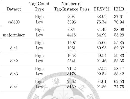
3.2 Comparison of Prediction Results of High Count Tags and Low Count Tags in Terms of False Negative Rate (in %) . . . 27

3.3 Some Example URLs with the Eight Example Tags as the High Count Tags in the Delicious Dataset . . . 29

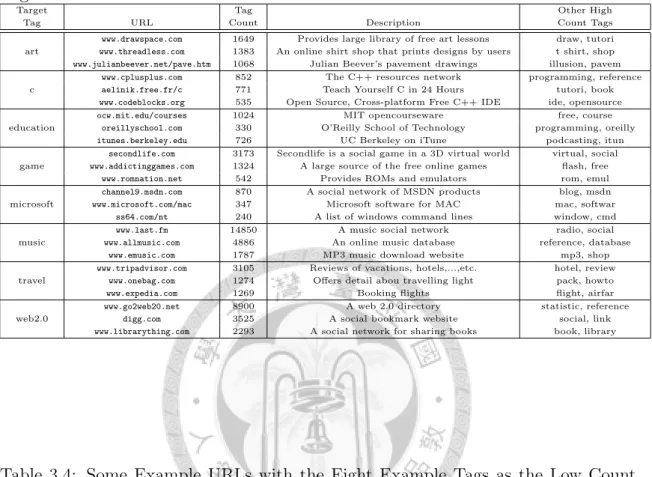
3.4 Some Example URLs with the Eight Example Tags as the Low Count Tags in the Delicious Dataset . . . 29

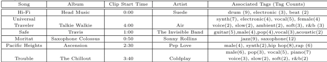
4.1 Some Examples of Audio Clips with Associated Tags Obtained from the MajorMiner Website . . . 34

4.2 Music Features Used in this Work . . . 39

(12)

4.3 Evaluation Results of MIREX 2009 Audio Tag Classiﬁcation on the MajorMiner Dataset. There are 12 submissions. Our submissions without and with pre-segmentation are denoted by NOS and SEG, respectively . . . 42

4.4 Evaluation Results of MIREX 2009 Audio Tag Classiﬁcation on the Mood Dataset. There are 12 submissions. Our submissions without and with pre-segmentation are denoted by NOS and SEG, respectively 42

4.5 Performance Rankings of Our Two Submissions to MIREX 2009 Au- dio Tag Classiﬁcation on Two Datasets . . . 43

4.6 Audio Tag Annotation and Retrieval Results of Diﬀerent Classiﬁers and Ensemble Methods on the MajorMiner Dataset (in %) . . . 45

4.7 Audio Tag Annotation and Retrieval Results of Cost-Sensitive Multi- Label Classiﬁcation Methods in Terms of Cost-Sensitive Metrics (in

%) . . . 46

4.8 Audio Tag Annotation and Retrieval Results of Cost-Sensitive Multi- Label Classiﬁcation Methods in Terms of Regular (Cost-Less) Metrics (in %) . . . 47

5.1 Statistics of the Multi-Label Datasets . . . 52

5.2 Selected Parameters k and M of GLE and RAk EL for the Multi-Label Datasets . . . 54

(13)

5.3 Experimental Results in Terms of Five Diﬀerent Evaluation Metrics.

The Numbers in Parentheses Represent the Rank of the Algorithm Among the Compared Algorithms. The Average Rank is the Average of the Ranks Across All Datasets. •/◦ indicates whether GLE is statistically superior/inferior to the compared algorithm (the pairwise t-test at the 5% signiﬁcance level). . . 56

5.4 Relative Improvement of GLE and Its Two Simpliﬁed Versions Over RAk EL in Terms of Five Diﬀerent Evaluation Metrics (In %) . . . 57

5.5 Experimental Results in Terms of Two Cost-Sensitive Evaluation Metrics. The Average Rank is the Average of the Ranks Across All Datasets. •/◦ indicates whether GLE is statistically superior/inferior to the compared algorithm (the pairwise t-test at the 5% signiﬁcance level). . . 60

6.1 Statistics of the BC and PE dataset . . . 81

6.2 Performance (AUC, in %) of Diﬀerent Patient-balanced Approaches on the BC Training Set (Cross-Validation) and Test Set. . . 83

6.3 Performance (AUC, in %) of Diﬀerent Patient-balanced Approaches on the PE Training Set (Cross-Validation) and Test Set. . . 83

(14)

List of Figures

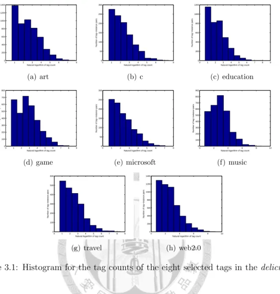
3.1 Histogram for the tag counts of the eight selected tags in the delicious data. . . 30

4.1 Work ﬂow of the proposed audio tag annotation and retrieval system. 37

4.2 Illustration of audio segmentation. . . 49

4.3 Work ﬂow of the classiﬁer ensemble used in the MIREX 2009 winning method. . . 50

5.1 Average relative improvement of GLE over RAk EL in terms of five different evaluation metrics with respect to different parameters k and M . . . 58

5.2 Experimental Results of GLE with Diﬀerent γ And ν in Terms of Five Diﬀerent Evaluation Metrics on The Scene Dataset. . . 61

5.3 Experimental Results of GLE with Diﬀerent γ And ν in Terms of Five Diﬀerent Evaluation Metrics on The Enron Dataset. . . 62

5.4 Experimental Results of GLE with Diﬀerent γ And ν in Terms of Five Diﬀerent Evaluation Metrics on The Cal500 Dataset. . . 63

(15)

5.5 Experimental Results of GLE with Diﬀerent γ And ν in Terms of Five Diﬀerent Evaluation Metrics on The Majorminer Dataset. . . 64

5.6 Experimental Results of GLE with Diﬀerent γ And ν in Terms of Five Diﬀerent Evaluation Metrics on The Medical Dataset. . . 65

5.7 Experimental Results of GLE with Diﬀerent γ And ν in Terms of Five Diﬀerent Evaluation Metrics on The Bibtex Dataset. . . 66

5.8 Experimental Results of GLE with Diﬀerent γ And ν in Terms of Five Diﬀerent Evaluation Metrics on The Dlc1 Dataset. . . 67

5.9 Experimental Results of GLE with Diﬀerent γ And ν in Terms of Five Diﬀerent Evaluation Metrics on The Dlc2 Dataset. . . 68

5.10 Experimental Results of GLE with Diﬀerent γ And ν in Terms of Five Diﬀerent Evaluation Metrics on The Dlc3 Dataset. . . 69

5.11 Experimental Results of GLE with Diﬀerent γ And ν in Terms of Five Diﬀerent Evaluation Metrics on The Dlc4 Dataset. . . 70

6.1 Histograms of the number of positive instances belonging to each patient on two medical image datasets . . . 77

(16)

Chapter 1 Introduction

Machine learning is the study of computer algorithms that improve automatically through experience [45]. It plays a key role in many areas of industry, finance, and science. Classification, is one of the most important task in machine learning. In the traditional classification problem, the computer is given a training set (x_i, y_i)^N_i=1, where x_i ∈ R^d is the feature vector of the i-th training sample and y_i is the class label. For binary classification, y_i ∈ {+1, −1} is the binary category label; while for multi-class classification, y_i ∈ {1, 2, . . . , K} denotes the K predefined classes.

The goal of these classification problems is to learn a classifier which maps data into the predefined classes. The learning procedure can be achieve by minimizing the expected misclassification cost on the training samples. The binary and multi- class classification problems are also called single-label classification problem, since each instance could be associated only one single label. In this proposal, we focus on a raising classification problem, called multi-label classification, which will be described below.

(17)

Instance Label Set

1 Rock,Guitar

2 Rock, Guitar, Drum 3 Rock, Guitar, Vocal 4 Country, Guitar 5 Rock, Guitar, Drum 6 R&B, Vocal 7 Country, Guitar

8 Vocal

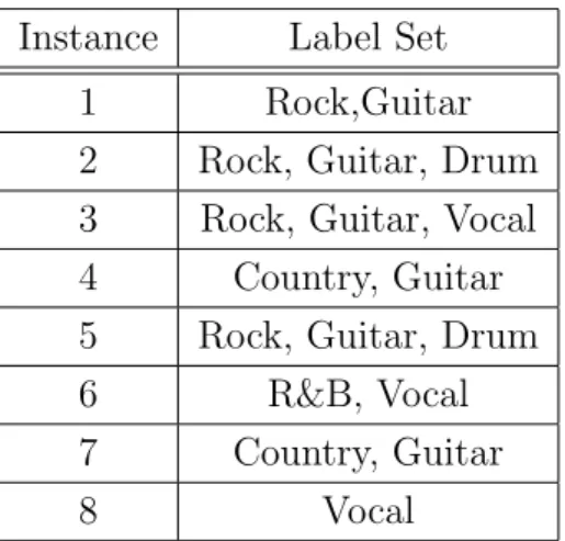
Table 1.1: An Example of Multi-Label Dataset for Music Tag Annotation

1.1 Multi-Label Classiﬁcation

Multi-label classiﬁcation has attracted a great deal of attention in recent years.

Different from single-label classification, in multi-label classification, an instance could be associated with a set of labels jointly. For example, in image classification, an image may possess several concepts, such as “sea” and “sunset”. Table 1.1 shows an example of multi-label dataset for music tag classification.

We define the problem of multi-label classification as below. Let Y ⊆ L = {λ1, λ₂, ..., λ_K}, which is a finite set of K possible labels. To facilitate the discussion, hereafter, Y is represented by a vector y = (y1, y₂, ..., y_K) ∈ {1, −1}^K, in which yj = 1⇔ λj ∈ Y, yj =−1 ⇔ λj ∈ Y. We denote the labels of the whole instances/ by Y ∈ R^N^×K, where the i-th row of Y is y_i; and denote the whole instances by X ∈ R^N^×d, where the i-th row of X is x_i. Given a training set (x_i, y_i)^N_i=1 that contains N samples, the goal of multi-label classification is to learn a classifier H :R^d→ 2^K such that H(x) predicts which labels should be assigned to an unseen sample x well.

Multi-label classiﬁcation methods can be grouped into two categories: algo- rithm adaptation and problem transformation [55]. The algorithm adaptation meth-

(18)

ods extend some specific learning algorithms for single-label classification to solve the multi-label classification problem. Zhang and Zhou [66] extended the famous back-propagation algorithm for multi-label learning (BPMLL). Some algorithms are extended from the instance-based learning, such as multi-label K-nearest neighbor (MLKNN) [67] and instance-based learning by logistic regression (IBLR) [10]. Elis- seeff and Weston [16] proposed an SVM-based method to minimize the ranking loss.

The problem transformation methods transform the multi-label classification problem to one or many single-label classification tasks. Binary relevance and label powerset are two popular problem transformation approaches. The binary relevance (BR) method trains a binary classifier for each label independently. Sun et al. [51]

proposed a two stage learning method to improve the binary relevance method based on hypergraph spectral learning. They exploited hypergraph spectral learning for feature transformation in the first stage and trained binary relevance classifiers in the second stage. The label powerset (LP) method treats each distinct combination of labels as a different class and, thus, treats the multi-label classification as a multi-class classification problem. In the next section, we introduce the concept of cost-sensitive single-label classification.

1.2 Cost-Sensitive Single-Label Classiﬁcation

Non-uniform misclassiﬁcation costs are very common in a variety of real-world applications. For example, in banking authentication, the cost of mistakenly authenticat- ing an intruder as a normal user is usually larger than that of mistakenly classifying a normal user as an intruder. The former type of mistakes might result in serious losses; while the later type of mistakes can be endured.

Current cost-sensitive learning research has been focused on binary or multi-

(19)

class classification [32, 35]. For cost-sensitive binary classification, Elkan proposed theoretical foundations [17]. Zadrozny et al. proposed a method called costing, based on rejection sampling method [65]. Costing can make common cost-less bi- nary classification algorithms cost-sensitive. Cost-sensitive multi-class classification research is more challenging than the binary one. MetaCost is the first cost- sensitive multi-class classification algorithm, which is based on a threshold-moving method [14]. Other approaches include re-weighting, sampling [70], and regression- based method [59].

Cost-sensitive classification starts from the assumption that the cost is given based on the application. “Where does cost come from? ” becomes an important practical issue [32]. One well-known application of cost-sensitive binary classification is the mailing campaign in KDD Cup 1998. The task is to send mail requests to potential donors to achieve maximum total profit. Different people might donate different amounts of money. Missing a major donor will results in large loss (cost), while sending requests to those who will not donate will also lose money. Beside the KDD Cup 1998 dataset, there are very few datasets with available cost information.

In this proposal, we study two real-world prediction tasks and link their data distribution to the cost information. The two tasks are medical image classification and social tag prediction. We study the medical image classification problem on the KDD Cup 2008 breast cancer (BC) dataset and the KDD Cup 2006 pul- monary embolism (PE) dataset. We observe a patient-imbalanced problem that has seriously hurt the generalization ability of the image classifier. We design several patient-balanced learning algorithms based on cost-sensitive binary classification.

The success of our patient-balanced learning methods has been proved by winning KDD Cup 2008.

For social tag prediction, consider that the tag count indicates the number of

(20)

users who have annotated the given resource with the tag. We believe the tag count information should be considered in automatic social tagging because the count reflects the confidence degree of the tag. Important, confident, and relevant tags (with respect to the resources, such as music tracks or websites) are usually assigned by many different users. We propose to treat the tag counts as the mis-classification costs and model the social tagging problem as a cost-sensitive learning problem. The experimental results in audio tag annotation and retrieval demonstrate that the cost- sensitive learning approaches outperform our winning method in Music Information Retrieval Evaluation eXchange (MIREX) 2009. The results on social bookmark prediction also demonstrate that our proposed method has better performance than other methods.

1.3 Cost-Sensitive Multi-Label Classiﬁcation

In addition to cost-sensitive single-label classification, we study a novel cost-sensitive multi-label classification (CSML) problem, which is a generalization of the traditional multi-label classification. In the CSML, the misclassification cost can be different for each instance-label pair and is given before the training process. For example, in image classification, the misclassification cost of the label “sunset” for an image whose subject is sunset should be higher than the misclassification cost of an additional label “gull”. More specifically, for each instance x_i, a misclassification cost c_j is coupled to each label λ_j belonging to the label set of that instance. We give a generalized definition as follow. We are given a training set (x_i, y_i, c_i)^N_i=1 that contains N samples, where the j-th component c_ij denotes the cost to be paid when the label yij is misclassified. More specifically, cij is a false negative cost when y_ij = 1, and a false positive cost when y_ij = −1. We denote the misclassification costs of the whole instances by C ∈ R^N^×K, where the i-th row of C is c_i. The goal of cost-sensitive multi-label classification is to learn a classifier H : R^d → 2^K such

(21)

that H(x) minimizes the expected misclassiﬁcation cost on an unseen sample x.

Since the problem is novel, no existing algorithm can be applied. In this work, we ﬁrst propose two general strategies based on the reduction technique.

The proposed strategies reduce the CSML problem to cost-sensitive single-label classification problem. In addition, we propose a basis expansions model for CSML, called Generalized k -Labelsets Ensemble (GLE), where a basis function is an LP classifier trained on a random k -labelset. The expansion coefficients are learned to minimize the global error between the prediction and the ground truth. GLE can also be used for traditional cost-less multi-label classification.

1.4 Proposal Organization

Now we briefly outline the contents of this proposal. In Chapter 2, we describe the proposed CSML methods. In Chapter 3, we study the effect of tag count in using multi-label classification for social tag prediction. The observation inspires us to formulate the social tag prediction task as a cost-sensitive multi-label classification problem by treating the tag counts as the misclassification costs. Chapter 4 presents our winning method of MIREX 2009 audio tagging competition and shows the experimental results of using CSML for audio tagging. The results demonstrate that the CSML approaches outperform our MIREX 2009 winning method. Chapter 5 contains the experimental results of GLE on both general multi-label classification datasets and cost-sensitive social tagging. Chapter 6 describes the patient- imbalanced problem in medical image classification and proposes patient-balanced learning algorithms. Chapter 7 concludes this proposal.

(22)

Chapter 2 Cost-Sensitive Multi-Label Classiﬁcation

In this chapter we start from reviewing some cost-sensitive single-label classification methods. Then, we propose two CSML methods: cost-sensitive stacking and cost-sensitive RAk EL, which are based on reducing CSML problem to several cost- sensitive single-label problems. Finally we propose Generalized k -Labelsets Ensem- ble (GLE) for both multi-label classification and cost-sensitive multi-label classification.

2.1 Cost-Sensitive Single-Label Classiﬁcation Meth- ods

In cost-sensitive binary classification, we are given a cost-sensitive training set (x_i, y_i, c_i)^N_i=1, where c_i ⊂ [0, ∞) is the misclassification cost. The goal of cost- sensitive classification is to learn a classifier f (x) that minimizes the expected cost as follows:

E[cI(f (x) ̸= y)], (2.1)

where I(·) is an indicator function that yields 1 if its argument is true, and 0 otherwise. In contrast, the expected cost in the traditional binary classiﬁcation is

(23)

deﬁned as:

E[I(f (x)̸= y)], (2.2)

which is a special case of (2.1) where all samples have an equal misclassification cost c. Many different cost-less binary classifiers can be extended to the cost-sensitive versions. In the following subsections, we describe two cost-sensitive binary classifiers: support vector machine (SVM) and AdaBoost.

2.1.1 Cost-Sensitive SVM

SVM finds a separating surface with a large margin between training samples of two classes in a high-dimensional feature space implicitly introduced by a computationally efficient kernel mapping [12]. The large margin implies good generalization ability according to statistical learning theory. We exploit a linear SVM classifier f (x) of the following form:

f (x) = w^Tx + b. (2.3)

In traditional SVM, the parameters w = (w₁, w₂, ..., w_d) and b can be learned by solving a minimization problem formulated as follows:

minw,b,ξ

1

2w^Tw + C

∑N i=1

ξ_i, s.t. y_i(w^Tx_i+ b) ≥ 1 − ξi

ξ_i ≥ 0

(2.4)

where ξ_i is the training error associated with instance x_i; C is a tuning parameter that controls the tradeoﬀ between maximizing the margin and minimizing the training error. Cost-sensitive SVM can be learned by modifying (2.4) to

minw,b,ξ

1

2w^Tw + C

∑N i=1

c_iξ_i, s.t. y_i(w^Tx_i+ b) ≥ 1 − ξi

ξ_i ≥ 0

(2.5)

where each cost c_i is associated with a corresponding training error term ξ_i.

(24)

2.1.2 Cost-Sensitive AdaBoost

AdaBoost [19] finds a highly accurate classifier by combining several base classifiers, even though each of them is only moderately accurate. It has been successfully used in applications such as music classification [3] and audio tag classification [15]. The decision function of the AdaBoost classifier takes the following form:

f (x) =

∑T t=1

α_th_t(x), (2.6)

where h_t(x) is the prediction score of a base classifier h_t given the feature vector x of a test sample; T is the number of base classifiers; and α_t can be calculated based on different versions of AdaBoost.

The base classiﬁers are learned iteratively. In the training phase, AdaBoost [52]

maintains a weight vector D_t for the training instances in each iteration and uses a base learner to ﬁnd a base classiﬁer h_t to minimize the weighted error according to Dt. In each iteration, the weight vector Dt is updated by

D_t+1(i) = D_t(i) exp(−αty_ih_t(x_i)) Zt

, (2.7)

where Z_t is a normalization factor that makes D_t+1 a distribution. We can increase the number of base learners iteratively and stop the training process when the generalization ability on the validation set does not improve. Cost-sensitive AdaBoost [52]

can be learned by modifying the update rule of weight vector D_t in (6.7) to

Dt+1(i) = D_t(i) exp(−αtc_iy_ih_t(x_i))

Z_t , (2.8)

where c_i is the cost of training instance x_i. We use decision tree as the base learner in this study.

(25)

2.2 Reducing Cost-Sensitive Multi-Label Classiﬁ- cation into Cost-Sensitive Single-Label Clas- siﬁcation

Reduction is a commonly used machine learning technique when the problem can not be solved by standard learning algorithms. In the research of traditional multi- label classification, a category of methods called problem transformation belongs to this kind of technique. It transforms the multi-label classification problem to one or many single-label classification tasks.

The binary relevance (BR) method is one of the popular problem transformation approaches. It trains a binary classifier for each label independently. For each label, the instances with/without the label will be treated as positive/negative examples for training the corresponding binary classifier. This manner inevitably loses the co-occurrence information of multiple labels that might be useful. Label correlation is an useful information for multi-label classification since some labels often co-occur. For example, in music tag annotation, a song with the “hip hop”

tag is more likely to be also annotated with “rap” than “jazz”, while a song with the “dance” tag is more likely to be also annotated with “electronic” than “guitar”.

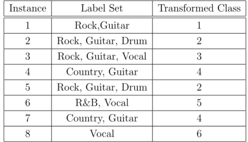
Label powerset (LP) [55] method is another problem transformation approach.

It treats each distinct combination of labels in the training set as a different class and, thus, treats the multi-label classification as a multi-class classification problem. Given a test instance, the multi-class LP classifier predicts the most probable class, which can be transformed to a set of labels. Table 2.1 shows an example of multi-label dataset with transformed multi-class label based on the concept of LP. However, one major concern for this model is that, when the number of labels increases, the number of potential classes increases proportionally, and each class will be associated with very few training instances. Moreover, LP can only

(26)

Table 2.1: An Example of Multi-Label Dataset with Transformed Multi-Class Labels Instance Label Set Transformed Class

1 Rock,Guitar 1

2 Rock, Guitar, Drum 2

3 Rock, Guitar, Vocal 3

4 Country, Guitar 4

5 Rock, Guitar, Drum 2

6 R&B, Vocal 5

7 Country, Guitar 4

8 Vocal 6

predict labelsets observed in the training data. In [56], a method called Random k -Labelsets (RAk EL) is proposed to overcome the drawback of the traditional LP method. RAk EL randomly selects a number of label subsets from the original set of labels and uses the LP method to train the corresponding multi-class classifiers. The final prediction of RAk EL is made by voting of the LP classifiers in the ensemble.

This method can not only reduce the number of classes, but also allow each class to have more training instances. Experimental results have shown an improvement of RAk EL over LP.

Inspired by the reduction methods for multi-label classiﬁcation, we propose two general strategies for reducing the CSML problem to cost-sensitive single-label classiﬁcation problem: a binary relevance based strategy and a label powerset based strategy. We describe these two methods in the following two subsections.

2.2.1 Cost-Sensitive Stacking

In this subsection, we propose a two-stage method called cost-sensitive stacking.

Stacking [63] is a method of combining the outputs of multiple independent classifiers for multi-label classification. In the first stage of cost-sensitive stacking, assume that the K labels are independent and we train cost-sensitive binary classifiers inde-

(27)

pendently. Then, we use the outputs of all binary classiﬁers, f₁(x), f₂(x), ..., f_K(x), as features to form a new feature set. Let the new feature be z = (z₁, z₂, ..., z_K).

We can use the new feature set together with the true label to learn the parameters w_kj of the stacking classiﬁers:

h_k(z) =

∑K j=1

w_kjz_j, (2.9)

where the weight w_kj will be positive if label j is positively correlated to label k;

otherwise, w_kj will be negative. The stacking classiﬁers can recover misclassiﬁed labels by using the correlation information captured in the weight w_kj.

2.2.2 Cost-Sensitive RAk EL

As mentioned in the beginning of Section 2.2, a method called Random k -Labelsets [58] is proposed to realize and improve the LP method. A k -labelset is a labelset R ⊆ L with |R| = k. RAkEL randomly selects a number of k-labelsets from L and uses the LP method to train the corresponding multi-label classiﬁers. Algorithms 1 and 2 describe the training and classiﬁcation processes of RAk EL, respectively.

The prediction of a multi-class LP classiﬁer g_m for sample x is denoted by g_m(x)∈ {1, 2, . . . , V }. Note that V will be much smaller than 2^k if the data is sparse. In Algorithm 2, q(g_m(x), j) is deﬁned as:

q(g_m(x), j) =





1 j ∈ Rm and j is positive in g_m(x),

−1 j ∈ Rm and j is negative in g_m(x),

∅ j /∈ Rm.

(2.10)

For example, when k = 2, the classes 1, 2, 3, and 4 correspond to (1, 1), (1,−1), (−1, 1), and (−1, −1), respectively. If label j is not included in Rm, q(g_m(·), j) is undeﬁned.

If label j corresponds to the ﬁrst label ofRm, q(1, j), q(2, j), q(3, j), and q(4, j) will be 1, 1,−1, and −1, respectively.

We extend RAk EL for cost-sensitive multi-label classiﬁcation. The extension is not straightforward since we are given a cost value for each label but RAk EL

(28)

Algorithm 1 The training process of RAk EL

• Input: number of models M, size of labelset k, set of labels L, and the training setD = (xi, y_i)^N_i=1

• Output: an ensemble of LP classiﬁers gm and the corresponding k -labelsets Rm

1. Initialize S ← L^k

2. for m← 1 to min(M,|L^k|) do

• Rm ← a k-labelset randomly selected from S

• train the LP classiﬁer gm based on D and Rm

• S ← S \ Rm

3. end

considers a set of labels as a class. Our idea is to train the cost-sensitive LP classiﬁer ˆ

g_mby transforming the cost of each label in a labelset to the total cost of the labelset.

The transformed cost ˆc_i of a training sample x_i for training ˆg_m is computed by

ˆ

ci(ci, y_i) =

{ ∑

j∈Rms.t. yij=1

c_ij if ∃j ∈ Rm s.t. y_ij = 1,

1 else,

(2.11)

where c_i is the cost vector mentioned in Section 1.3. Therefore, we can obtain the multi-class training sample with the associated cost, (x_i, ˆy_i, ˆc_i), for training the LP classifier, where ˆyi ∈ {1, 2, . . . , V } is the class value and ˆci is the cost to be paid when the class of this instance is misclassified. We use the multi-class SVM as the LP classifier in this study, and employ the one-versus-one strategy [33] in cost-sensitive multi-class classification.

2.3 Generalized k -Labelsets Ensemble (GLE)

As RAk EL is considered an ensemble-based multi-label classification method, it has to follow the theory states [13] that “a necessary and sufficient condition for an ensemble of classifiers to be more accurate than any of its individual members is if the

(29)

Algorithm 2 The classiﬁcation process of RAk EL

• Input: number of models M, a test sample x, an ensemble of LP classiﬁers g_m, and the corresponding k -labelsets Rm

• Output: the multi-label classiﬁcation vector r = (r1, r₂, ..., r_K) 1. for j ← 1 to K do

(a) rj = 0, n = 0

(b) for each g_m, if j ∈ Rm do

• rj = r_j + q(g_m(x), j)

• n = n + 1 (c) end

(d) rj = ^r_n^j 2. end

individual classifiers are accurate and diverse”. Here the term accurate implies that such classifier has a lower error rate than random guessing. In RAk EL, the diversity of classifiers is achieved by randomly selecting label subsets. The major limitation of this kind of ensemble method is that such “committee-of-diverse-experts” heuristics do not directly optimize for the learning objective. In contrast, AdaBoost.M2 [19] is an ensemble method for single-label classification, which directly optimizes a learning objective. Breiman [4] shows that the training procedure of AdaBoost is a form of gradient optimization to minimize the objective function J (F ) =∑

iexp(−yiF (x_i)), where y_i is the class label of the instance x_i and F (·) is a hypothesis classiﬁer of AdaBoost. Both theoretical and experimental results show the superiority of Ad- aBoost. Our work tries to follow a similar idea to improve RAk EL by re-designing the learning function to optimize a global error objective function.

Another limitation of RAk EL is that it assumes every base classifier in the ensemble is equally important. However, such assumption is problematic because the individual LP classifiers are trained on different randomly selected k -labelsets, some of them may have worse predictive performance than others or can be even

(30)

redundant. Researchers have shown that properly determining the weights of the base classifiers in an ensemble can improve the prediction performance [6, 19]. For example, in AdaBoost, the coefficient αt of a base classifier ft(x) is determined analytically and is proportional to the predictive performance of f_t(x). We believe that learning the weights of base classifiers in an ensemble can improve the prediction performance for multi-label classification.

Inspired by the success of the LP-based methods, we presents a novel machine learning model for multi-label classiﬁcation using the idea of basis expansions model [21, Chapter 5] of the following form:

H(x) =

∑M m=1

β_mh_m(x), (2.12)

where the basis functions h_m(x) exploit the LP classifiers trained on random k - labelsets and β_m are their coefficients. In general, the basis expansions model treats the classifiers h_m(x) as dictionary functions and uses the linear combination of these functions to approximate the target classifier during the learning procedure [21, Chapter 5]. Intuitively, given sufficient dictionary functions, the basis expansions model is a flexible representation for the target multi-label classifier.

In our proposed GLE, the coefficients β_m are learned to minimize the global error between the prediction of H(x) and the ground truth. The coefficients β_m of the corresponding base classifiers h_m(x) become more significant for base classifiers with better performance, and are not redundant given others. Another interpretation of our method is from the Bayesian framework. The GLE can be considered as a kind of Bayesian model combination, that is, P (Yi|x) = ∑

mP (Yi|x, hm)P (h_m), where the Yi is a predicted label set. In this aspect, the coeﬃcients β_m are approximating the prior probabilities P (hm) for the model hm.

In the following subsections, we describe the proposed GLE for multi-label classiﬁcation, review the concept of exploiting hypergraph for multi-label classiﬁca-

(31)

tion, and extend GLE for cost-sensitive multi-label classiﬁcation.

2.3.1 GLE for Multi-Label Classiﬁcation

Similar to RAk EL, GLE first trains M LP-based classifiers using randomly selected k -labelsets from the original set of labels. Then, GLE uses the base classifiers as dictionary functions and learns a linear combination of these functions. Algorithms 3 and 4 describe the training and classification processes, respectively. The weight coefficients β for the base classifiers are learned by solving a minimization problem formulated as follows:

minβ 1

2||Y − ∑^M

m=1

βmQm||²F +^γ₂||β||²2

+^ν₂trace ((∑M

m=1

β_mQ_m )T

L (∑M

m=1

β_mQ_m ))

,

(2.13)

where || · ||F is the Frobenius norm of a matrix, L is the normalized hypergraph Laplacian, and Q_m ∈ R^N×Kis a transformed prediction of g_mwhich will be described in more detail later. The ﬁrst term in the objective function aims to minimize the global error between the prediction of H(x) and the multi-label ground truth Y . The second term is a two-norm regularization term of the coeﬃcients β. The third term is a hypergraph regularization term.

The prediction of a multi-class LP classiﬁer, g_m, for a sample x is denoted by g_m(x) ∈ {1, 2, . . . , Z}. Note that Z will be much smaller than 2^k if the data is sparse. Similar to RAk EL, the i, j-th element in Q_m is calculated by q(g_m(x_i), j), which is deﬁned as:

q(g_m(x_i), j) =











1, if j ∈ Rm

and j is positive in gm(xi),

−1, if j ∈ Rm

and j is negative in g_m(x_i), 0, if j /∈ Rm.

(2.14)

For example, when k = 2, the classes 1, 2, 3, and 4 correspond to (1, 1), (1,−1), (−1, 1), and (−1, −1), respectively. If label j is not included in Rm, q(gm(xi), j) is 0. If

(32)

Algorithm 3 The training process of GLE

• Input: number of models M, size of labelset k, learning parameters γ and ν, set of labelsL, and the training set D = (xi, y_i)^N_i=1

• Output: an ensemble of LP classiﬁers gm, the corresponding k -labelsets Rm

and coeﬃcients βm

1. Initialize S ← L^k

2. for m← 1 to min(M,|L^k|) do

• Rm ← a k-labelset randomly selected from S

• train the LP classiﬁer gm based on D and Rm

• calculate a transformed prediction of gm using (6.2)

• S ← S \ Rm

3. end

4. Learn β using (2.19)

label j corresponds to the first label of Rm, q(1, j), q(2, j), q(3, j), and q(4, j) will be 1, 1,−1, and −1, respectively. We note that the function q(gm(x), j) is used to generate the hm(x) in the final classifier (2.12) by gathering the predictions on all labels j.

The trade-off between fitting the training data and regularization can be con- trolled by the parameters γ and ν. A larger parameter γ will lead to smoother coef- ficients β. The hypergraph Laplacian L∈ R^N×N captures the high order labelling relationship among different instances. Following the spectral graph theory [11, 51], our idea behind the hypergraph regularization term is that the prediction on two instances, that is, two rows in ∑_M

m=1βmQm, should be similar if they have high similarity according to the hypergraph.

To solve the optimization problem (2.13), we start from rewriting the ﬁrst term of the objective function by vectorizing Q_m and Y . We denote the prediction of the base classiﬁers by ˆQ ∈ R^(L·N)×M whose columns are vectorized from Q_m by

(33)

Algorithm 4 The classiﬁcation process of GLE

• Input: number of models M, a test sample x, an ensemble of LP classiﬁers g_m, and the corresponding k -labelsets Rm and coeﬃcients β_m

• Output: the multi-label classiﬁcation vector r = (r1, r₂, ..., r_K) 1. for j ← 1 to K do

(a) rj = 0

(b) for each g_m, if j ∈ Rm do

• rj = r_j + β_m· q(gm(x), j) (c) end

2. end

reshaping Q_m into R^(L^·N); and vectorize Y into ˆY ∈ R^(L^·N). Then, the ﬁrst term of the objective function can be rewritten as ¹₂|| ˆY − ˆQβ||²2. To further simplify the third term of the objective function, we let Q_m,j be the j-th column vector in Q_m. We perform operations on the third term as follows:

ν 2trace

((∑M m=1

β_mQ_m )T

L (∑M

m=1

β_mQ_m ))

= ^ν₂trace





β^TP_1,1β · · · β^TP_1,Lβ ... . .. ... β^TP_L,1β · · · β^TP_L,Lβ





= ^ν₂

∑L j=1

β^TP_j,jβ

(2.15)

where P_i,j ∈ R^M^×M is generated as

P_i,j =





Q^T_1,iLQ1,j · · · Q^T1,iLQM,j

... . .. ... Q^T_M,iLQ1,j · · · Q^TM,iLQM,j



 . (2.16)

Let∑L

j=1P_j,j in (2.15) be denoted as ρ, the loss function in (2.13) can be rewritten as

L(β) = 1

2( ˆY − ˆQβ)^T( ˆY − ˆQβ) + γ

2β^Tβ + ν

2β^Tρβ. (2.17)

(34)

We take derivatives of equation (2.17) with respect to β and set them equal to zero,

∂L

∂β =− ˆQ^TY + ˆˆ Q^TQβ + γˆ · Iβ + ν

2(ρ + ρ^T)β = 0. (2.18) where I is the identity matrix. Hence, the optimization problem (2.13) has a unique solution β^∗:

β^∗ = ( ˆQ^TQ + γˆ · I + ν

2(ρ + ρ^T))⁻¹Q ˆˆY . (2.19) The computational cost of training GLE depends on the training speed of the LP base classiﬁer. We note that the matrix to be inverted in (2.19) is a M -dimensional square matrix and typically the number of models M is set from 15 to 250. Hence, solving such equation is computationally feasible and learning β does not increase much overhead.

2.3.2 Multi-Label Learning with Hypergraphs

Hypergraph is a generalization of the traditional graph in which an edge can connect arbitrary non-empty subsets of the vertex set [1]. We denote a hypergraph by G = (V, E), where V is the vertex set and E is the edge set, where each edge is a subset of V . Traditional graph is a special case of the hypergraph, in which every edge connects exactly two vertices, and is also called “2-graph”. Given a multi-label dataset, the instances with their labels can be represented as one single hypergraph.

More speciﬁcally, the vertex is a data point and the hyperedge is a label that connects the instances associated with it. A normalized hypergraph Laplacian L ∈ R^{|V |×|V |} is a commonly used technique for capturing the relationship among nodes in the hypergraph and has been used in spectral clustering [69]. Sun et al. proposed the hypergraph spectral multi-label learning algorithm [51] to learn a low-dimensional feature transformation W , such that the data points sharing many common labels tend to be close to each other in the transformed space. The optimization problem

(35)

for learning W is formulated as follows:

minW trace(W^TXLX^TW )

s.t. W^TXX^TW = I, (2.20)

where W^TX is the transformed data.

In this paper, we exploit the relation information encoded in the hypergraph Laplacian L in a different manner. We add a hypergraph Laplacian regularizer into the objective function for learning the coefficients in the ensemble. There are several different methods for learning the normalized hypergraph Laplacian matrix, but Agarwal et al. have shown that these methods lead to similar results [1]. In this paper, we use the clique expansion algorithm [1, 51] for calculating the normalized hypergraph Laplacian.

The clique expansion algorithm constructs a 2-graph from the original hypergraph by replacing each hyperedge with a clique, that is, maintaining an edge for each pair of vertices in the hyperedge. For a hypergraph, the vertex-edge incidence matrix J ∈ R^{|V |×|E|} is deﬁned as: J (v, e) = 1 if v ∈ e and 0 otherwise. We de- note the weight associated with the hyperedge e by w(e). We denote the diagonal matrix whose diagonal entries are w(e) by W_H. In the application of hypergraph for multi-label classiﬁcation, the weights are set to uniform for each hyperedge. We denote the vertex degree in the expanded 2-graph by dc(u), where u is a vertex of the 2-graph, and denote the diagonal matrix whose diagonal entries are d_c(u) by D_c. The normalized hypergraph Laplacian can be calculated by

L = I − Dc^−1/2J WHJ^TD_c^−1/2. (2.21)

2.3.3 GLE for Cost-Sensitive Multi-Label Classiﬁcation

GLE can also be extended for cost-sensitive multi-label classiﬁcation. We follow the same training and classiﬁcation procedures as shown in Algorithms 3 and 4,

(36)

and modify the objective function for learning the coefficients β in (2.13). Recall that the first term in the objective function of (2.13) is the global error between the multi-label classifier prediction, ∑M

m=1βmQm, and the multi-label ground truth Y . We modify it to a cost-weighted global error by multiplying the global error with the multi-label misclassification cost matrix C. The optimization problem of learning the coefficients β for cost-sensitive multi-label classification can then be formulated as follows:

minβ 1

2||C ◦(

Y − ∑^M

m=1

βmQm

)||²F +^γ₂||β||²2

+^ν₂trace ((∑M

m=1

β_mQ_m )T

L (∑M

m=1

β_mQ_m ))

,

(2.22)

where ◦ is the dot product of two matrices. Similarly, the optimization problem (2.22) has a unique solution β^∗,

β^∗ = (

C◦ ( ˆQ^TQ) + γˆ · I +ν

2(ρ + ρ^T) )₋₁

Q ˆˆY . (2.23)

(37)

Chapter 3 A Study on the Eﬀect of Tag Count in Using Multi-Label Classiﬁcation for Social Tag Prediction

Tags are free text labels annotated on data in different format, such as images, music tracks, and websites. In some cases, the tags are objective and assigned by experts, such as part-of-speech tagging, or semantic role labelling. In other cases, the tags are more or less subjective while different persons might compose different tag sets for an object. In the Web 2.0 era, there are more and more online services that allow or even encourage users to tag objects such as images, or music tracks, and consequently create a large set of subjective tagging data. The emergence of human computing [64] also creates mass of opportunity for users to tag media. In general, we call such tagging behavior “collective tagging” and the subjective tags produced through such process “collective tags”. The collective tags usually capture different aspects of the content. For example, the types of music tags may contain artist, genre, mood, and instrumentation. Given a feature representation for the content of the resources, some previous researches [15, 40] assumed that the tags are independent and, thus, transformed the social tag prediction problem into many