護理人員生涯需求與醫院生涯發展方案差距對離職傾向之影響－以工作滿意為中介變項

全文

(1)經濟與管理論叢(Journal of Economics and Management), 2009, Vol. 5, No. 2, 167-186. The Co-Movement and Long-Run Relationship between Inflation and Stock Returns: Evidence from 12 OECD Countries Chih-Chuan Yeh* Department of Finance, The Overseas Chinese Institute of Technology, Taiwan. Ching-Fang Chi Department of Banking and Finance, Tamkang University, Taiwan This paper carries out the methodology suggested by Den Haan (2000) to investigate the co-movement of inflation and real stock returns using quarterly data from OECD countries. We confirm the existence of both short-run and long-run relationships between inflation and real stock returns, regardless of whether the underlying time series data are purely I(0), purely I(1), or mutually co-integrated. Moreover, we use the confidence interval approach introduced by Stock (1991) to further point out the ambiguity in unit root tests. However, our results support the existence of an inverse co-movement and long-run relationship between these two variables in 12 OECD countries. That is, an increase in inflation depresses real stock prices. This evidence is consistent with both the inflation illusion hypothesis and with the classical view that stock returns should be undervalued to reflect the imbalance in the tax treatment of inventory. Keywords: inflation, stock returns, co-movement, ARDL-ECM JEL classification: C33, G21, O16. 1. Introduction. The linkage, if any, between inflation and real stock returns has received considerable attention over the last half century. Starting with the pioneering work Received November 17, 2008, revised March 23, 2009, accepted March 10, 2009. * Correspondence to: Department of Finance, The Overseas Chinese Institute of Technology, Taiwan. E-mail: robert@ocit.edu.tw. We wish to thank to the anonymous referees for helpful comments and suggestions..

(2) 168. Chih-Chuan Yeh and Ching-Fang Chi. of Fisher (1930), real stock returns were suggested as a good potential hedge against inflation, often referred to as the Fisher effect. This paper empirically reinvestigates the co-movement between inflation and real stock returns. We implement the analysis by exploring the distinct impacts of inflation on real stock returns at different time horizons. The issue may be of crucial importance in advancing our understanding of stock markets, and in providing benchmarks for decision-making about asset allocation. The relationship between stock returns and inflation has been the subject of extensive research. For decades, it was generally believed that inflation and stock returns exhibited a negative correlation. Often, some type of theoretical hypothesis was mentioned to rationalize a negative co-movement between real stock returns and inflation rates [see, e.g., Fama and Schwert (1977), Fama (1981), Ram and Spencer (1983), and Stulz (1986)]. There are different views on hypotheses that support the negative relationship between inflation and real stock returns. Modigliani and Cohn’s (1979) hypothesis (i.e., the inflation illusion hypothesis) explains that the real effect of inflation is caused by money illusion.1 If the nominal interest rate including the inflation premium is higher, then stock prices are undervalued. That the relationship between inflation and real stock prices eliminates the money illusion is puzzling. Feldstein’s (1980) tax-effects hypothesis argues that inflation erodes real stock returns due to imbalanced tax treatment of inventory and depreciation caused by a decrease in real after-tax profit by inflation. Fama’s (1981) hypothesis, based on the money demand theory, suggests that a negative correlation is not a causal relationship, but a spurious result of the dual effect. The reason is because when inflation is negatively related to real economic activity and there is a positive association between real activity and stock returns, the negative relationship between inflation and stock returns holds. Caporale and Jung (1997) argue against Fama’s conjecture by contending that real stock returns are inversely related to inflation, even when controlling for economic output. Ritter and Warr (2002) use a residual income model to show that valuation errors of leveraged stocks in the presence of inflation cause depressed stock prices. Therefore, decreasing inflation triggered the bull market in the U.S. from 1982 to 1999. 1 There are few empirical studies, including Sharpe (2002), Asness (2000, 2003), Campbell and Vuolteenaho (2004) and Cohen et al. (2005), that provide evidence in support of the money illusion hypothesis..

(3) The Relationship between Inflation and Stock Returns. 169. Recently, however, the sign of the relationship between real stock returns and inflation has been called into question. In a noteworthy study, Rapach (2002) reports that long-run inflation neutrality exists in the stock markets of 16 OECD countries.2 He adopts the method provided by King and Watson (1997) under the restraints in which data satisfies integration and co-integration properties and reports that the long-run Fisher effect exists because long-run real stock returns do not respond to a permanent inflation shock. Thus, the empirical evidence of the relationship between inflation and real stock returns is puzzling. Additionally, some authors employ the bivariate ARIMA model, the bivariate vector autoregression (VAR) model, or the co-integration test to determine the inflation and real stock returns relationship in the long-run. See, for example, Lee (1992), who finds no causal relationship between stock returns and inflation during the postwar period. In this paper, we use the co-movement approach of Den Haan (2000) to investigate the short-run relationship and the autoregressive distributed lag (ARDL) bound test methodology introduced by Pesaran et al. (2001) to investigate the existence of a long-run relationship between inflation and real stock returns using 12 industrialized OECD countries. We do not care whether both of the included variables in levels are purely I (0) , purely I (1) , or mutually co-integrated before entering the co-movement and ARDL bound test. So, not only co-movement but also the ARDL regression can avoid the problem of different integrated orders. Therefore, we use four kinds of unit root tests and the confidence interval method introduced by Stock (1991) to confirm whether the results are mixed. Except for real stock returns in Australia, Ireland, Japan, and the United States, we find that the two level variables among the remaining countries include stationary and non-stationary results. The estimations of the largest autoregressive root in the confidence intervals of Stock (1991) mostly include unity, except for the inflation in New Zealand. The aim of this paper is to characterize and analyze the co-movement and the long-run relationship between inflation and real stock returns in a large group of OECD countries. The empirical results show that 12 OECD countries display significantly negative co-movement between inflation and real stock returns in the short-run. Moreover, a small group of countries (Australia, France, Ireland, and the. 2 A similar argument can be found in Gallagher and Taylor (2002) and Kim (2003), which is supported by compelling empirical evidence..

(4) 170. Chih-Chuan Yeh and Ching-Fang Chi. Netherlands) do not exhibit a long-run equilibrium between these two variables. Section 2 outlines the econometric methodology related to the dynamic and equilibrium relationship separately. Section 3 describes and reports the data sources and main empirical results. Finally, conclusions drawn from this study are presented in Section 4.. 2. Methodology. 2.1 Measuring Correlations at Different Forecast Horizons with VAR Forecast Errors This section describes the methodology suggested by Den Haan (2000) for measuring correlations at different forecast horizons. There are two restrictions on using the unconditional correlation coefficient to investigate the dynamic short-run relationship. First, it is effective only for stationary variables. Second, it does not account for important information about dynamic characteristics in the co-movement of variables. To solve the above restrictions on the orders of integration and lost information, we adopt the correlations of VAR forecast errors at different horizons introduced by Den Haan (2000) to examine the co-movement of inflation and the real stock returns. Let us consider an N × 1 vector of random variables, X t . The vector X t is allowed to contain any combination of stationary processes and processes that are integrated of arbitrary order. Let X t = ( S t , π t )' , that is N = 2 , where S t and π t are real stock returns with inflation at time t , respectively. We want to illustrate the co-movement between inflation, π t , and real stock returns, S t ; X t must include at least π t and S t . Consider the following VAR in levels with polynomial time trend: J. X t = μ + β t + γ t 2 + ∑ ϕ j X t− j + ε t , j =1. (1). where μ , β and γ are the intercept matrices, and ϕ j is a 2 × 2 matrix of coefficients for lag j . The terms ε t follow a white noise process – that is, they must be serially uncorrelated but can be correlated with each other. J is the total.

(5) The Relationship between Inflation and Stock Returns. 171. number of lags. We denote the k-period ahead forecast and the k-period ahead forecast error of the variables S t by Et ( S t + k ) and S tue, t + k , respectively. Let the unexpected forecast error in the real stock returns forecasted k-periods ahead at time t to be denoted by: S tue, t +k = S t +k − Et ( S t +k ) .. (2). Here, Et ( S t + k ) is the expected value of the k -period ahead real stock returns at time t , and S t +k is the actual value at time (t + k ) Similarly, we can define. π tue, t +k = π t +k − Et (π t +k ) . Then, the covariance coefficient and correlation coefficient between S tue, t + k and π tue, t +k are denoted by COV (k ) and COR(k ) , respectively. Den Haan (2000) points out that if all variables included in X t are stationary, then COR(k ) will converge to the unconditional correlation coefficient between S t and π t as k goes to infinity. If some variables in X t are non-stationary,. then their statistics might not converge, but can be estimated consistently for a fixed k . However, this approach need not be concerned with the order of integrated. variables included in X t , but only with the situation in which the number of lags must be large enough to guarantee that ε t is serially uncorrelated and not integrated. Following Den Haan (2000), the unexpected forecast errors forecasted k -periods ahead at time t , S tue, t + k and π tue, t +k , are considered in the VAR. framework. The covariance and correlation coefficients are obtained from the VAR coefficients. Using the correlation coefficient of the forecast error to analyze the relationship between inflation and real stock returns at a particular horizon k is possible – that is, we can observe the co-movements between inflation and real stock returns in the short-run.. 2.2. The ARDL Bounds Testing Approach. Previous studies use econometric methods to investigate the long-run relationships between level variables. Most of these analyses have been based on the use of co-integration approaches. Engle and Granger (1987) and Johansen’s (1991, 1996) methods have been adopted and estimated as well. In addition, Fisher and Seater (1993) provide a bivariate ARIMA framework under important restrictions depending on the orders of integration. And Caporale and Jung (1997) demonstrate.

(6) 172. Chih-Chuan Yeh and Ching-Fang Chi. the existence of an inverse relationship between inflation and real stock returns while controlling for the growth rate of real output and inflation. All of these methods focus on cases in which the underlying variables are integrated of order one. Later, Rapach (2003) uses the approach of King and Watson (1997) to test the same topic. The included variables in the structural VAR approach of King and Watson (1997) are required to be at least I (1) , but need not co-integrate. In this study, we reassess the issue of whether inflation and real stock returns are co-integrated by using the newly developed bounds testing procedure analyze level relationships within an autoregressive distributed lag (ARDL) framework. This renewed interest is due, in large part, to advances in the development of time series methodologies for studying non-stationary data. Given the uncertainty concerning the time series properties of the variables in question, we view this methodology as the most appropriate for this context. For illustrative purposes, this section describes the approach suggested by Pesaran et al. (2001) to solve restrictions on the orders of integration. This approach does not require inflation and underlying real stock returns to be I (0) or I (1) . Let us consider a 2 × 1 vector of random variables, Yt , in an unrestricted VAR in levels. The vector Yt also can include either stationary or non-stationary time series. Consider the following VAR in levels without the time trend, and eq. (1) can be rewritten as: p. Yt = α + ∑ β j Yt − j + υ t .. (3). j =1. However, notice that Yt = ( S t , π t +1 )' , and where S t is the real stock price at time t and π t +1 is the inflation at time t + 1 . The matrix α contains two intercept terms, and β j is a 2 × 2 matrix of coefficients for lag j . In order to investigate the effect of inflation on real stock prices in the long-run, we implement the Pesaran et. al. (2001)’s bounds procedure to extend eq. (1) into the conditional ARDL model from the VECM, and follow Rapach (2002)’s formula: p −1. q −1. j =1. j =1. ΔS t = λ + ϕ S t −1 + δπ t + ∑ β S , j ΔS t − j + ∑ β π , j Δπ t +1− j + ωΔπ t +1 + ξ t ,. (4). where λ is a drift term, and the coefficients of two level terms, ϕ and δ , reveal the long-run relationship. The number of lags in the differential terms are p and.

(7) The Relationship between Inflation and Stock Returns. 173. q , respectively, and determined by Akaike information criterion (AIC) or. Schwarz’s information criterion (BIC) in an ARDL( p, q ) model. Finally, ξ t is generated from a white-noise process. Following Pesaran et al. (2001), if the long-run relationship between inflation and real stock prices exists, the null hypothesis H 0 : ϕ = δ = 0 must be rejected. In other words, the test statistics exceed an asymptotic upper critical value for the F-statistic. Otherwise, if the test statistics fall below an asymptotic upper critical value for the F-statistic, we cannot reject the null hypothesis of no long-run relationship. If, however, the statistics fall within their respective bounds, the inference would be indeterminate. Notice that the asymptotic distribution of this F-statistic is not standard, regardless of whether inflation and the real stock price are stationary. As for the estimators of the parameters in eq. (4), we can use ordinary least squares (OLS) to estimate and test the existence of the long-run relationship through the asymptotic critical value tables by Pesaran et al. (2001). These tables provide two asymptotic distributions, upper and lower bounds, respectively, for corresponding to the regression, which considers unrestricted intercepts and no trends.3 The upper value is obtained when the regressors are purely I (1) but the lower value is obtained when the regressors are purely I (0) . Because. ΔS t − j = Δπ t +1 = 0 holds, we can obtain the reduced form from a steady-state of eq. (4), described by: S t = θ 0 + θ1π t +1 + ε t ,. (5). where θ 0 = −λ ϕ , θ1 = δ ϕ and ε t follows stationary process.. 3. Data and Empirical Results. 3.1. Data Description. The data used in this paper consist of quarterly observations of the nominal stock index and consumer price index for 12 industrialized OECD countries: Australia, Canada, Finland, France, Germany, Ireland, Italy, Japan, Netherlands, New Zealand, Spain, and United States. The data series are from the International Monetary Fund’s 3. Table CI reports detailed asymptotic critical value bounds for the F-statistic in Pesaran et al. (2001)..

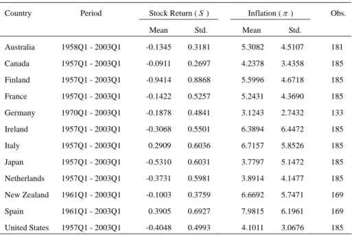
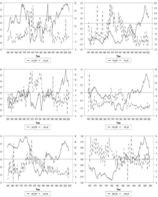
(8) 174. Chih-Chuan Yeh and Ching-Fang Chi. International Financial Statistics (IFS) provided by the Taiwan AREMOS database. The exact length of sample periods for each country is reported in Table 1. Except for the starting dates for Australia, Spain, Germany and New Zealand, the remaining countries start from 1957Q1 to 2003Q1. The natural logarithm of actual changes in the consumer price index (CPI) represents inflation. Additionally, we take the natural logarithm of the nominal stock index divided by the consumer price index (CPI) to represent real stock returns. Table 1 reports basic statistics for inflation and real stock returns for each country. The mean values of inflation in our samples range from 3.12% to 7.98%. As shown, Spain has the highest average inflation (7.98%) while Germany has the lowest average inflation (3.12%). However, all the inflation variability is from 2.74% (Germany) and 6.45% (Ireland). Figure 1 shows plots of the level trend between inflation rates (the dashed line) and real stock returns (the solid line) for each of the 12 countries. Table 1: Basic statistics Country. Period. Stock Return ( S ). Inflation ( π ). Mean. Std.. Mean. Obs.. Std.. Australia. 1958Q1 - 2003Q1. -0.1345. 0.3181. 5.3082. 4.5107. 181. Canada. 1957Q1 - 2003Q1. -0.0911. 0.2697. 4.2378. 3.4358. 185. Finland. 1957Q1 - 2003Q1. -0.9414. 0.8868. 5.5996. 4.6718. 185. France. 1957Q1 - 2003Q1. -0.1422. 0.5257. 5.2431. 4.3690. 185. Germany. 1970Q1 - 2003Q1. -0.1878. 0.4841. 3.1243. 2.7432. 133. Ireland. 1957Q1 - 2003Q1. -0.3068. 0.5501. 6.3894. 6.4472. 185. Italy. 1957Q1 - 2003Q1. 0.2909. 0.6036. 6.7157. 5.8526. 185. Japan. 1957Q1 - 2003Q1. -0.5310. 0.6031. 3.7797. 5.1472. 185. Netherlands. 1957Q1 - 2003Q1. -0.3731. 0.5981. 3.8914. 4.1477. 185. New Zealand. 1961Q1 - 2003Q1. -0.1003. 0.3759. 6.6692. 5.7471. 169. Spain. 1961Q1 - 2003Q1. 0.3905. 0.6927. 7.9815. 6.1961. 169. United States. 1957Q1 - 2003Q1. -0.4048. 0.4993. 4.1011. 3.0676. 185. Notes: 1. The data set was taken from the International Monetary Fund's International Financial Statistics provided by the Taiwan AREMOS database. 2. The real stock return (S) equals the natural logarithm of the nominal stock index divided by the consumer price index. Inflation (π) equals the quarterly rate calculated as the percentage change in the logarithm of consumer price index..

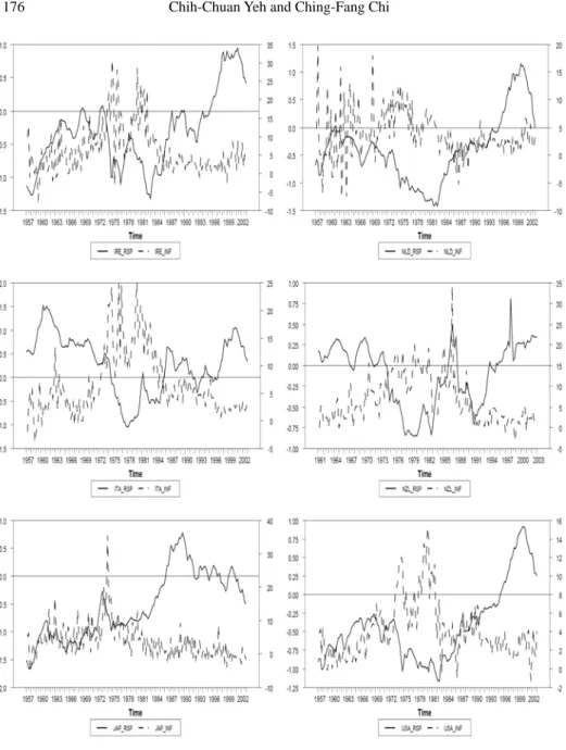
(9) The Relationship between Inflation and Stock Returns. 175. From Figure 1, we obtain the inverse trend between real stock returns and inflation for most counties. The results show that higher inflation erodes stock returns, leading to lower real stock returns in the long-run. However, the level trend of a positive short-term co-movement between two variables exists only for Spain, the Netherlands, and Japan.. Figure 1: The level trend between inflation (dashed lines) and real stock returns (solid lines)..

(10) 176. Chih-Chuan Yeh and Ching-Fang Chi. Figure 1: The level trend between inflation (dashed lines) and the real stock returns (solid lines). (continued). 3.2. The Unit Root Results. We start our empirical analysis by examining the stochastic properties of the time.

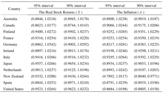
(11) The Relationship between Inflation and Stock Returns. 177. series. Whether VAR or ARDL models are used to investigate the co-movement or long-run relationship between inflation and real stock returns, they are required for diagnostic checks that ensure that no variable is integrated of order more than one. It is more important that in the long-run relationship, the linear (co-integrating) combination of included variables needs to be I (0) in structural econometric methods, such as in an error-correction model (ECM) introduced by Engle and Granger (1987) or the Johansen (1988). For the 12 countries considered, we first investigate the integration properties of S t and π t using Ng and Perron (2001) unit root tests, which are variants of the well-known Dickey and Fuller (1981) and Phillips and Perron (1988) tests, respectively. Both tests use GLS-detrending to maximize power and modified information criteria to select the lag truncation parameter in an effort to minimize size distortions. Table 2 reports the results for the ADF, PP, and Ng-Perron tests for our data. What emerges from this evidence is a confirmation of the complex nature of the dynamic properties of both variables, with a mixture of I (0) and I (1) series found across the sample periods. As shown, except for real stock returns in Australia, Ireland, Japan, and United States, which are I (1) , and inflation in the Netherlands and United States being I (0) , there are mixed results. In addition, Bahmani-Oskooee (1998) suggests that the uncertain results from different tests depend on the power of unit root tests. Moreover, Stock (1991) suggests that only unit root tests and point estimations of the largest autoregressive root are unsatisfying because good information appears to be consistent with the observed data.4 Therefore, we report the asymptotic confidence intervals developed from Stock (1991) under 95% and 90% confidence levels in Table 3. We find that only the largest root of the inflation in United States does not include unity under the 90% confidence level, and it significantly rejects the null hypothesis of non-stationarity.. 4 Campbell and Mankiw (1987) and Cochrane (1988) support the notion that the confidence intervals for the largest autoregressive root are more useful than unit root tests alone..

(12) 178. Chih-Chuan Yeh and Ching-Fang Chi. Table 2: Unit root test results Country. ADF. PP. Ng-Perron MZ a. S Australia. π. π. S. -2.1815 -2.5070. -2.1878. MZ t. π. S. -6.9492. *** ***. -4.8132 -7.9334. -7.1092 *. π. S *. -1.8683*. -1.4262 *. Canada. -2.2368 -1.9472. -2.0617. -5.4972. -5.3348. -1.8648. Finland. -1.5062 -2.3544. -0.7729. -5.5815***. -6.2073*. -10.2920**. -1.5478. France. -1.7206 -2.0055. -1.4005. -5.4293***. -6.2466*. -1.797. -1.7411*. -0.9113. ***. -6.0769. *. *. -1.6092. -1.6754. Germany. -1.6715 -2.0531. -1.3430. -8.2930. Ireland. -2.2717 -2.1132. -1.6553. -8.5140*** ***. -6.4373 -0.9362. Italy. -1.7722 -1.7194. -1.8098. -3.7745. Japan. -1.8939 -2.2281. -1.7612. -9.4025***. Netherlands. -2.2591 -1.9607. -1.3678 -12.3831. ***. New Zealand -1.8871 -3.3634**. -1.8684. -4.6475***. Spain. -1.4947. -9.3811. -0.9813. -4.1485***. -2.4445 -1.9946. United States -1.0913 -2.8365*. *. -21.6328 -5.8357*. ***. -5.1859. -1.7419. -5.6175. -0.6845. -1.806. -1.7908. -8.2407**. -0.5891. -0.7635. -2.2374**. -1.6378** *. -0.9339 -1.9466*. ***. -2.7465. -3.2559. -4.0611. -1.6878*. -14.7971*** -1.9969. -1.6021. -1.1657 -1.4250. -2.7188*** -0.9977. -19.3441*** -0.3698. -3.1099***. Notes: 1. “S” equals the real stock returns and “π” equals the inflation rate. 2. ***, **, and * indicate significance at the 1%, 5% and 10% level, respectively. 3. The Augmented Dickey-Fuller (ADF) test statistic is estimated, and its critical values are from Dickey and Fuller (1981). 4. PP indicates the test statistic of the Phillis-Perron unit root test. 5. MZ a and MZ t indicate the test statistic of the Ng-Perron unit root test. Table 3: The results of confidence intervals Country. 95% interval. 90% interval. The Real Stock Returns ( S ). 95% interval. 90% interval. The Inflation ( π ). Australia. (0.8846, 1.0218). (0.8965, 1.0178). (0.8900, 1.0228). (0.9019, 1.0187). Canada. (0.8623, 1.0177). (0.8744, 1.0143). (0.9066, 1.0244). (0.9175, 1.0206). Finland. (0.9400, 1.0272). (0.9502, 1.0237). (0.9252, 1.0265). (0.9351, 1.0229). France. (0.9316, 1.0254). (0.9410, 1.0220). (0.9253, 1.0254). (0.9350, 1.0219). Germany. (0.8862, 1.0342). (0.9002, 1.0292). (0.8217, 1.0281). (0.8383, 1.0225). Ireland. (0.8897, 1.0216). (0.9013, 1.0176). (0.9198, 1.0246). (0.9298, 1.0211). Italy. (0.9416, 1.0266). (0.9516, 1.0232). (0.9295, 1.0264). (0.9392, 1.0229). Japan. (0.9557, 1.0266). (0.9654, 1.0234). (0.8934, 1.0237). (0.9053, 1.0196). Netherlands. (0.9013, 1.0237). (0.9125, 1.0198). (0.8993, 1.0242). (0.9107, 1.0203). New Zealand. (0.9332, 1.0280). (0.9436, 1.0244). (0.7892, 1.0117). (0.8040, 0.9771). Spain. (0.8844, 1.0253). (0.8971, 1.0210). (0.8791, 1.0239). (0.8919, 1.0196). United States (0.9523, 1.0264) (0.9623, 1.0232) (0.8684, 1.0198) (0.8805, 1.0158) Notes: The asymptotic confidence intervals developed from Stock (1991) under 95% and 90% confidence levels..

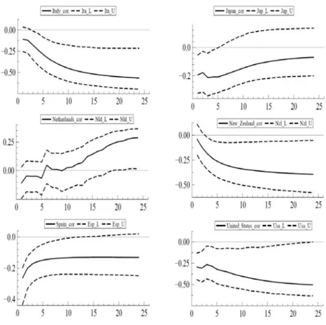
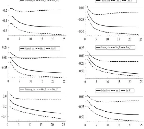
(13) The Relationship between Inflation and Stock Returns. 3.3. 179. Co-Movement between Inflation and the Real Stock Returns. In short-run dynamic relationships, we use the procedures from Section 2.1 to analyze the co-movement between inflation and real stock returns in 12 OECD countries. The co-movement between inflation and real stock returns is described using the correlation coefficients of VAR forecast errors at different forecast horizons, as proposed in Den Haan (2000). Correlation coefficients of forecast errors are estimated based on VARs that only include inflation and real stock returns. Intuitively, the covariance and correlation coefficients of inflation and real stock returns are estimated by measuring the difference between the actual (realized) values and the corresponding expected (forecast) values, which are forecast errors, from one quarter to 24 quarters of forecast periods. A disadvantage of using the intuitive method is that the sample size is shortened when the forecast horizon is too long. Correlation coefficients of forecast errors are also estimated from the VAR forecast model. Here, we only investigate the estimations from the VARs where the data have been levels of the variables – that is, without imposing the unit root restriction. First, the number of lags is determined based on Akaike information criterion (AIC) and Schwarz information criterion (BIC) in a VAR forecast errors model. The simulated data set is generated by 2,500 replications from bootstrapping, and then confidence bands are calculated for the estimated correlations at the 90% confidence level.5 The results are robust, so we only report part of AIC in Figure 2. Figure 2 displays a set of graphs, one for each country analyzed. Each graph shows the estimated correlation coefficients, and 10% - 90% confidence bands constructed using bootstrap methods. We find that, in most countries, except for in Japan, the Netherlands, and Spain, co-movement relationships are negative under the 90% confidence level in the short-run. In other words, inflation erodes real stock returns in the short-run.. 5 See Den Haan (2000) and Den Haan and Sumner (2004) for a detailed discussion. This paper also documents estimation of the correlation coefficients and the confidence bands. The bootstrap procedure is called BOOT written in the RATS program. The BOOT instruction is used to draw entry numbers with replacement from the estimated errors of the VAR..

(14) 180. Chih-Chuan Yeh and Ching-Fang Chi. Figure 2: Correlation coefficients from no unit root imposed VAR forecast errors model for inflation and real stock returns. Moreover, based on empirical evidence in which economic activities inversely relate to inflation, our results can be reasonably interpreted to support the Modigliani et al. (1979)’s inflation illusion hypothesis. When the nominal interest rate distributed by the high inflation premium is higher, stock returns are undervalued. The negative values in those countries become increasingly small as forecast horizons increase. The relationship between the real stock price and inflation in Japan and the Netherlands is almost insignificant, but positive co-movement in the Netherlands arises when the forecast horizon increases to 20-period forecast horizons. We observe the dynamic relationship in the VAR forecast error model, and report that negative and significant co-movement relationships exist clearly in the short-run. We then apply the ARDL model without.

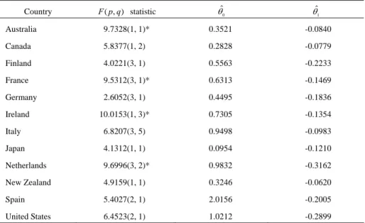
(15) The Relationship between Inflation and Stock Returns. 181. I(0) or I(1) problems to investigate the long-run equilibrium relationship between the real stock price and inflation.. Figure 2: Correlation coefficients from no unit root imposed VAR forecast errors model for inflation and real stock returns. (continued). 3.4. The Long-Run Level Relationship. From eq. (4), we estimate using OLS and test the joint null hypothesis of δ = ϕ = 0 , which stands for no long-run relationship between the real stock price and inflation, by calculating F-statistics. After setting the maximum lag order at 12, we report results for the specifications in the ARDL( p, q) model in Table 4 that minimizes the AIC value to select the optimal lag order. For Australia, France, Ireland, and the Netherlands, F-statistics are more than the 1% asymptotic upper critical value of.

(16) 182. Chih-Chuan Yeh and Ching-Fang Chi. 7.84, and significantly reject the null hypothesis of no long-run relationship, regardless of whether S t and π t are I (0) or I (1) . The remaining countries do not exhibit long-run equilibrium relationships, because F-statistics are less than the 1% asymptotic lower critical value of 6.84. Table 4: Asymptotic critical value bounds for a level relationship. F ( p, q) statistic. θˆ0. θˆ1. Australia. 9.7328(1, 1)*. 0.3521. -0.0840. Canada. 5.8377(1, 2). 0.2828. -0.0779. Finland. 4.0221(3, 1). 0.5563. -0.2233. France. 9.5312(3, 1)*. 0.6313. -0.1469. Germany. 2.6052(3, 1). 0.4495. -0.1836. 10.0153(1, 3)*. 0.7305. -0.1354. Italy. 6.8207(3, 5). 0.9498. -0.0983. Japan. 4.1312(1, 1). 0.0954. -0.1210. Netherlands. 9.6996(3, 2)*. 0.9832. -0.3162. New Zealand. 4.9159(1, 1). 0.3246. -0.0620. Spain. 5.4027(2, 1). 2.0156. -0.2005. Country. Ireland. United States 6.4523(2, 1) 1.0212 -0.2899 Notes: 1. Upper and lower bounds for critical value are 7.84 and 6.84 under the 1% level, respectively. 2. If the F-statistic is above an upper asymptotic critical value, the null hypothesis of no long-run relationship is rejected under the 1%(*) level. If the F-statistic is below a lower asymptotic critical value, the null hypothesis of no long-run relationship is accepted. Otherwise, if the F-statistic is between these two bounds the result is inconclusive. 3. The estimated coefficients, θˆ0 and θˆ1 , are obtained from eq. (5).. Briefly, θˆ0 are estimates of constants in the long-run level relationship. Only the estimates in Spain and the United States are over unity. However, the θ1 in eq. (5) describes how the real stock returns at time t are affected by inflation at time t + 1 in the long-run. The θˆ values in Australia, France, Ireland, and the 1. Netherlands are negative and account for the existence of the long-run, inverse response of real stock returns to changes in inflation. Otherwise, all estimates of θ1 are negative, regardless of the existence of a long-run equilibrium relationship. Therefore, the above results are consistent with Modigliani and Cohn’s (1979) hypothesis and Feldstein’s (1980) hypothesis. They argue that an increase in inflation depresses real stock returns. Those results echo our findings in Figure 1..

(17) The Relationship between Inflation and Stock Returns. 183. Our results are also consistent with Caporale and Jung’s (1997) empirical results, which showed that, even after controlling for output shocks, inflation still has a significantly negative impact on real stock returns. Our results do not support Rapach’s (2002) conjecture that indicates that long-run neutrality between real stock returns and inflation exists –that is, an increase in inflation trends do not erode real stock returns.. 4. Conclusions. This paper investigates the co-movement (short-run) and long-run equilibrium relationships between real stock returns and inflation in 12 industrialized OECD countries. In an attempt to provide an empirically based explanation for such a connection, we use Den Haan’s (2000) and Pesaran’s et al. (2001) approach to explore the short-run and long-run correlation between these two variables. There are two innovative advantages that improve constraints in integration of order for time series data in these two econometric methods. First, we can test for the existence of dynamic co-movement and long-run relationships in levels between variables, even incorporating both I (0) and I (1) variables. Second, a better description of the dynamic relationship between variables is obtained than when the focus is only on the unconditional correlation coefficient. The empirical results show that a large portion of the sample of 12 OECD countries displays negative co-movement between inflation and stock returns in the long-run. More importantly, we find that inflation in Australia, France, and Ireland are inversely related to real stock returns, regardless of whether variables are in the co-movement or long-run equilibrium relationship. Except for the co-movement relationship in Japan and Spain, the remaining countries exhibit significantly negative relationships in both co-movement and long-run relationships, even if they do not have a long-run equilibrium.. References Asness, C. S., (2000), “Stocks versus Bonds: Explaining the Equity Risk Premium,” Financial Analysts Journal, 56, 96-113..

(18) 184. Chih-Chuan Yeh and Ching-Fang Chi. Asness, C. S., (2003), “Fight the Fed Model: The Relationship between Future Returns and Stock and Bond Market Yields,” Journal of Portfolio Management, 30, 11-24. Bahmani-Oskooee, M., (1998), “Do Exchange Rates Follow a Random Walk Process in Middle Eastern Countries?” Economics Letters, 58, 339-344. Campbell, J. Y. and N. G. Mankiw, (1987), “Are Output Fluctuations Transitory?” The Quarterly Journal of Economics, 102, 857-880. Campbell, J. Y. and T. Vuolteenaho, (2004), “Inflation Illusion and Stock Prices,” American Economic Review, 94, 19-23. Caporale, T. and C. Jung, (1997), “Inflation and Real Stock Prices,” Applied Financial Economics, 7, 265-266. Cochrane, J. H., (1988), “How Big is the Random Walk in GNP?” Journal of Political Economy, 96, 893-920. Cohen, R. B., C. Polk, and T. Vuolteenaho, (2005), “Money Illusion in the Stock Market: The Modigliani-Cohn Hypothesis,” The Quarterly Journal of Economics, 120, 639-668. Den Haan, W. J., (2000), “The Comovement between Output and Prices,” Journal of Monetary Economics, 46, 3-30. Den Haan, W. J. and S. W. Sumner, (2004), “The Comovement between Real Activity and Prices in the G7,” European Economic Review, 48, 1333-1347. Dickey, D. A. and W. A. Fuller, (1981), “Likelihood Ratio Statistics for Autoregressive Time Series with a Unit Root,” Econometrica, 49, 1057-1072. Engle, R. F. and C. W. J. Granger, (1987), “Co-Integration and Error Correction: Representation, Estimation, and Testing,” Econometrica, 55, 251-276. Fama, E. F., (1981), “Stock Returns, Real Activity, Inflation, and Money,” American Economic Review, 71, 545-565. Fama, E. F. and G. W. Schwert, (1977), “Asset Returns and Inflation,” Journal of Financial Economics, 5, 115-146. Feldstein, M., (1980), “Inflation and the Stock Market,” American Economic Review, 70, 839-847. Fisher, I., (1930), The Theory of Interest, New York: MacMillan. Fisher, M. E. and J. J. Seater, (1993), “Long-Run Neutrality and Superneutrality in an ARIMA Framework,” American Economic Review, 83, 402-415..

(19) The Relationship between Inflation and Stock Returns. 185. Gallagher, L. A. and M. P. Taylor, (2002), “The Stock Return-Inflation Puzzle Revisited,” Economics Letters, 75, 147-156. Johansen, S., (1988), “Statistical Analysis of Cointegration Vectors,” Journal of Economic Dynamics & Control, 12, 231-254. Johansen, S., (1991), “Estimation and Hypothesis Testing of Cointegration Vectors in Gaussian Vector Autoregressive Models,” Econometrica, 59, 1551-1580. Johansen, S., (1996), Likelihood Based Inference on Cointegration in the Vector Autoregressive Model, New York: Oxford University Press. Kim, J.-R., (2003), “The Stock Return-Inflation Puzzle and the Asymmetric Causality in Stock Returns, Inflation and Real Activity,” Economics Letters, 80, 155-160. King, R. G. and M. W. Watson, (1997), “Testing Long-Run Neutrality,” Federal Reserve Bank of Richmond Economic Review, 83, 69-101. Lee, B.-S., (1992), “Causal Relations among Stock Returns, Interest Rates, Real Activity, and Inflation,” Journal of Finance, 47, 1591-1603. Modigliani, F. and R. Cohn, (1979), “Inflation, Rational Valuation and the Market,” Financial Analysts Journal, 35, 24-44. Ng, S. and P. Perron, (2001), “Lag Length Selection and the Construction of Unit Root Tests with Good Size and Power,” Econometrica, 69, 1519-1554. Pesaran, M. H., Y. Shin, and R. J. Smith, (2001), “Bounds Testing Approaches to the Analysis of Level Relationships,” Journal of Applied Econometrics, 16, 289-326. Phillips, P. C. B. and P. Perron, (1988), “Testing for a Unit Root in Time Series Regression,” Biometrika, 75, 335-346. Ram, R. and D. E. Spencer, (1983), “Stock Returns, Real Activity, Inflation, and Money: Comment,” American Economic Review, 73, 463-470. Rapach, D. E., (2002), “The Long-Run Relationship between Inflation and Real Stock Prices,” Journal of Macroeconomics, 24, 331-351. Rapach, D. E., (2003), “International Evidence on the Long-Run Impact of Inflation,” Journal Money, Credit, and Banking, 35, 23-48. Ritter, J. R. and R. S. Warr, (2002), “The Decline of Inflation and the Bull Market of 1982-1999,” Journal of Financial and Quantitative Analysis, 37, 29-61. Sharpe, S. A., (2002), “Reexamining Stock Valuation and Inflation: The.

(20) 186. Chih-Chuan Yeh and Ching-Fang Chi. Implications of Analysts’ Earnings Forecasts,” Review of Economics and Statistics, 84, 632-648. Stock, J. H., (1991), “Confidence Intervals for the Largest Autoregressive Root in U.S. Macroeconomic Time Series,” Journal of Monetary Economics, 28, 435-459. Stulz, R. M., (1986), “Asset Pricing and Expected Inflation,” Journal of Finance, 41, 209-223..

(21)