雙光子聚合技術應用於大範圍之產品設計與製造

(1)

國立臺灣大學工學院機械工程學研究所碩士論文

Department of Mechanical Engineering College of Engineering

National Taiwan University Master Thesis

雙光子聚合技術應用於大範圍之產品設計與製造 Design and Fabrication of Large Scale 3D Objects by

Two-Photon Polymerization Technology

湯期文 Qi-Wen Tang

指導教授：鍾添東博士 Advisor: Tien-Tung Chung, Ph.D.

中華民國 106 年 7 月

July, 2017

(2)

口試委員審定書

(3)

致謝

感謝指導教授鍾添東老師，除了指導專業知識和研究方法之外，也提供相當充足的研究資源，使我能專心投入研究。感謝共同參與研究計畫的各位教授們，

王安邦教授，許聿翔教授提供研究的方向，並在口試時給予論文的指導，給予許多寶貴的建議，使本論文更加完備。感謝劉昭沅博士提供雙光子技術上的指導以及撰寫學術文章的技巧。以上許多前輩的指導，使我這兩年的研究生涯中收穫良多並能如期完成此論文，在此獻上我最真摯的敬意與感謝。

感謝機械工程學研究所電腦輔助繪圖實驗室的全體夥伴，感謝維德學長、嘉榮學長、慶雄學長、尚哲學長、浩宇學長在我研究所期間協助解決實驗室相關問題。感謝智濠學長、永健學長、以磬學長傳承實驗室的雙光子製造技術並在協助解決研究上遇到的難題。感謝學弟妹郁寬、志承、承林、子皓、育菁、安禧，與我一起努力奮鬥以及體驗研究生活。也感謝顏家鈺教授實驗室、張所鋐教授實驗室、王安邦教授實驗室、許聿翔教授實驗室以及廖英智教授實驗室的協助與配合，

提供專業的研究設備，使研究得以順利進行。

感謝父母、哥哥以及親人在這一路上的關心與支持，使我無需問生活擔憂，

支持我度過每一個難關。感謝好友們的鼓勵與陪伴，在研究生活上相互扶持。最後感謝一路上支持我、幫助過我的每一個人，在此獻上我最衷心的感謝，謝謝大家。

(4)

雙光子聚合技術應用於大範圍之產品設計與製造摘要

本文研究以雙光子聚合技術應用於大尺寸三維產品的設計與製造。本雙光子聚合製造系統使用 130 kHz 高重複率之 Nd:YAG 雷射、三維壓電平台，並搭配放大倍率 50 倍、數值孔徑 0.8 的物鏡製作細胞培養基質與疏水性結構。藉由直接聚焦雷射於樹脂而不通過玻片，再以蜂巢式製作方法避免結構倒塌，製作出具有曲面結構的細胞培養基質以及具有特定表面粗糙度的細胞培養基質，予以提供造骨細胞遷徙之相關研究。再者，本研究根據 Cassie & Baxter 模型，製作出不同設計參數的疏水結構並量測其接觸角，將其疏水結構製作於 PDMS 晶片之微流道中以進行二項流產生測試。比較兩者有無加入疏水性結構之流態分佈圖，可發現疏水性結構可有效減小環狀流之面積。最後，本研究建構了一組大範圍雙光子製造系統，其包含 4 瓦高功率飛秒雷射、振鏡掃描系統，壓電驅動平台以及傾斜校正平台。藉由整合以上元件，可製作邊長 1 毫米的方形光柵以及直徑 3 毫米的台灣大學校徽。

關鍵字：雙光子聚合、雙光子吸收、飛秒雷射、振鏡掃描系統、疏水性結構、細胞遷移、表面粗糙度

(5)

Design and Fabrication of Large Scale 3D Objects by Two-Photon Polymerization Technology

Abstract

This thesis studies on design and fabrication of large scale 3D objects by two-photon polymerization. The established TPP fabrication system equipped with 130 kHz repetition rate Nd: YAG laser, 3D piezostage, and 50x microscope objective with NA=0.8 were used to fabricate substrates for cell migration and hydrophobic structures. With laser beam directly focused on resin without through coverslip and honeycomb bulkhead method for avoiding structures collapse, the substrates with curvature surface and the substrates with different surface roughness regions were fabricated and provided for studying the migrating behavior of human osteosarcoma cells. Moreover, according to the Cassie & Baxter model, hydrophobic structures with different design parameters were fabricated. The hydrophobic structure with droplets contact angle greater than 90 degree is made inside the channel of PDMS chip for emulsion generation. Comparing the flow regimes map of PDMS chip with and without hydrophobic structures, the annular flow region becomes narrower with hydrophobic structure. In addition, a large scale TPP fabrication system including 4W high power femtosecond laser, galvanometer scanner, piezo-driven translation stage and tilt stage was established. With the integration of these components, large-scale optical grating with size of 1mm x 1mm and the logo of National Taiwan University with 3mm diameter can be manufactured successfully.

Keywords: two-photon polymerization, two-photon absorption, femtosecond laser, galvanometer scanner, hydrophobic structure, cell migration, roughness control

(6)

LIST OF FIGURES

Fig. 1-1 Comparison between TPA and single-photon absorption generated by a focused laser beam: (a) Schematic diagram of a focused laser beam, (b) Single-photon absorption per transverse plane, and (c) Two-photon absorption

per transverse plane [10] ... 2

Fig. 1-2 Illustration of comparing two photon excitation with single photon [11] ... 2

Fig. 1-3 Feature sizes of lines fabricated between two closely transposed supports, with scanning speed 700 µm/s. [1] ... 3

Fig. 1-4 Schematic of ascending scan method [14] ... 4

Fig. 1-5 SEM images of suspended crossbar structure with 1.25 NA objective lens [13] ... 5

Fig. 1-6 Laser fabrication setup and millimeter sized scaffold consisting of 30 x 30 hexagons fabricated [15] ... 6

Fig. 1-7 The schematic and SEM image of tube structure [6] ... 6

Fig. 1-8 The setup of system based on based on galvanometric mirror scanner [16] .... 7

Fig. 1-9 The scanning galvanometer systems and the projections of the voxels with different incident angles [17] ... 7

Fig. 1-10 Structures fabrication via TPP technology applied in diversified fields ... 8

Fig. 1-11 Bio-structure fabrication by TPP ... 9

Fig. 1-12 Cell morphology on different roughness of Ti surface [20] ... 10

Fig. 1-13 Surface characterization of three different types of surfaces [21]... 10

Fig. 1-14 Effect of surface microstructure and surface energy on differentiation of MG63 osteoblast-like cells [21] ... 11 Fig. 2-1 Intensity distribution of Gaussian beam and the definition of laser beam full

(9)

Fig. 2-2 The interface of PSF Lab software. ... 15

Fig. 2-3 A voxel fabrication by TPP ... 16

Fig. 2-4 Schematic diagram of TPP micro-fabrication [25] ... 17

Fig. 2-5 LM slicing method for Taipei 101 building ... 18

Fig. 2-6 The schematic of fabrication, immersion and the final desired product [26]. 18 Fig. 2-7 User interface of the slicing process ... 19

Fig. 2-8 Schematic diagram of TPP micro fabrication system based on 3D piezostage ... 20

Fig. 2-9 Hardware setup with piezostage ... 21

Fig. 2-10 Carbon dioxide pressure-temperature phase diagram ... 22

Fig. 2-11 Manual critical point dryer K850 ... 23

Fig. 2-12 Comparison between natural drying and critical point drying ... 23

Fig. 3-1 The experimental setups of rapid TPP system ... 26

Fig. 3-2 The system set-up of two-photon polymerization system based on galvanometer scanner... 27

Fig. 3-3 Beam deflection via galvanometer scanners ... 28

Fig. 3-4 The different between optic lenses and F-theta lenses ... 29

Fig. 3-5 The maximum size of grating made with the rapid TPP system ... 30

Fig. 3-6 Part of scanning path data ... 30

Fig. 3-7 The laser marking sample of RTC5 ... 31

Fig. 3-8 Scan head control timing during jump command and mark command ... 32

Fig. 3-9 Defect caused by incoordination between scanner and z-stage ... 32

Fig. 3-10 The code for delay between layer and layer ... 33

Fig. 3-11 Illustration of the code for delay between layer and layer ... 33

Fig. 3-12 Voxel fabrication with OrmoComp® ... 34

(10)

Fig. 3-13 Line fabrication with suspended bridge method and OrmoComp® ... 35

Fig. 3-14 Illustration for the mechanism of the tilt stage ... 36

Fig. 3-15 SEM image of 51 x 51 grating and NTU Logo ... 36

Fig. 3-16 OrmoComp® setup for higher structures bounded by the tape on coverslip ... 37

Fig. 3-17 tube structures fabricated with 116.67μm inner diameter, 140.01μm outer diameter and 1mm height (laser power = 4W, exposure time = 10ms) ... 37

Fig. 3-18 SEM image of large scale structures ... 38

Fig. 3-19 The SEM image of large scale structures with grating base ... 39

Fig. 4-1 Mechanical response between PI P-611 and P-615 with exposure time 5ms [29] ... 41

Fig. 4-2 The CAD model and SEM image of the testing grating ... 41

Fig. 4-3 Diagram of length error versus various grating size. ... 42

Fig. 4-4 Form error calibration of PI P-615 piezostage with size of 270 µm x 180µm name cards ... 42

Fig. 4-5 Exposure strategy and spherical aberration due to refraction at interfaces of materials with the indices n = 1 (air), n’= 1.515 (glass), and n’’ = 1.538 (resin) . 43 Fig. 4-6 Schematic view of the different exposure strategies. ... 44

Fig. 4-7 CAD model of Taipei 101 with size 193 µm x 40 µm x 40 µm. ... 45

Fig. 4-8 Taipei 101 fabricated with different exposure strategies. ... 45

Fig. 4-9 Design parameters of curvature substrate ... 47

Fig. 4-10 Slicing strategies of different patrs of curvature substrate ... 47

Fig. 4-11 Curvature substrates fabricated with TPP ... 47 Fig. 4-12 Top view of fabricating sequence with the unsorting scanning paths (the

(11)

Fig. 4-13 CAD model of substrates with different curvature surface ... 49 Fig. 4-14 Substrate fabrication with shell model ... 49 Fig. 4-15 CAD model of substrate with honeycomb bulkhead method ... 50 Fig. 4-16 Substrates with different curvature surface and different scanning direction

... 50 Fig. 4-17 Illustrative model to show the voxel-induced roughness [31] ... 51 Fig. 4-18 Plates fabricated with different voxel distance (fabrication parameters: laser power = 4mW, exposure time = 4ms, fabrication time = 138 minutes) ... 52 Fig. 4-19 Confocal microscope images of plate with V.D. = 0.7 ... 52 Fig. 4-20 The relation between voxel distance and roughness ... 53 Fig. 4-21 Side view of roughness controlled surface with difference slice methods .. 54 Fig. 4-22 SEM images of roughness controlled surfaces (fabrication parameters: laser power = 4mW, exposure time = 4ms, processing time = 153 minutes) ... 54 Fig. 4-23 Illustration of HCP concept of roughness controlled surface ... 55 Fig. 4-24 The results fabricated with different voxel arrangement (fabrication parameters: laser power = 4mW, exposure time = 4ms) ... 55 Fig. 4-25 CAD of substrates with different roughness regions ... 56 Fig. 4-26 SEM images of substrates fabricated with different roughness regions (fabrication parameters: exposure time = 4ms, laser power = 4mW, processing time = 3 hours for each one) ... 57 Fig. 4-27 Images of migrating cells on the fabricated substrates [33] ... 57 Fig. 4-28 Illustration of HCP concept of roughness controlled surface(Arrows point from 0.4 μm to 1.3μm) [34] ... 58 Fig. 5-1 The side view of vapor pockets trapped between the structures and the droplet. θa is the advancing contact angle, d is the depth of droplet wetting into

(12)

vapor pocket, θd is the angle defined with d and structure, ω is the angle

between structure and coverslip ... 60

Fig. 5-2 The CAD model and the parameters of the hydrophobic structure ... 61

Fig. 5-3 Product of 3 x 3 hydrophobic structure ... 62

Fig. 5-4 Schematic drawing of system for array fabrication ... 62

Fig. 5-5 21 x 21 hydrophobic structure with 600μm 600μm cover area ... 63

Fig. 5-6 92 x 80 hydrophobic structure with 2.5mm x 2.2mm cover area... 63

Fig. 5-7 Plane structure with 2.06mm x 2.24mm cover area and 29nm roughness ... 64

Fig. 5-8 Measurement of contact angle with different surface ... 64

Fig. 5-9 Hydrophobic structure with b = 9.2μm ... 65

Fig. 5-10 Contact angles of four different surface with 2μL droplet ... 65

Fig. 5-11 The PMMA chip for emulsion generation ... 66

Fig. 5-12 The PDMS chip for emulsion generation ... 67

Fig. 5-13 The images of hydrophobic structure applied on PDMS chip ... 68

Fig. 5-14 Representative flow patterns of two-phase flow in PDMS chip with hydrophobic structure. (a) cover area of the hydrophobic structure; (b) slug flow; (c) droplet flow; (d) annular flow ... 68

Fig. 5-15 Flow regimes map for flow patterns in the chip (…the transition line from slug flow to annular flow) ... 70

Fig. 5-16 The images of one line hydrophobic structure applied on PDMS chip ... 71

Fig. 5-17 The flow regimes map of physical upper limit test ... 72

Fig. A-1 System diagram of scann head part ... 87

Fig. A-2 System diagram of laser part ... 87

(13)

LIST OF TABLE

Table 3-1 Major equipments and characteristics ... 27

(14)

NOMENCLATURES

v frequency of the incident light 𝐼₀ maximum intensity per unit area 𝐼_𝑡ℎ threshold energy intensity

r beam radius

𝜔₀ beam radius of the laser waist

P average power

FWHM full width half maximum

𝑣_𝑎 voxel width

𝑣_𝑏 voxel height

𝜔_𝑥𝑦 beam radius along the radial axis 𝜔_𝑧 beam radius along the optical axis

𝑀² beam quality

d penetration depth of focus 𝑑^′ thickness of coverslip

∆ z coordinate of each voxel n refraction index

𝑅_𝑧 surface roughness

𝑆₀ scanned area

𝑓(𝑥, 𝑦) height at each point 𝑧₀ average height

a length of cube

h height of cube

(15)

𝜃_𝑐 apparent contact angle

𝜃_𝑠 intrinsic contact angle on the original smooth surface 𝑓_𝑠 area fractions of vapor on the surface

ℎ_𝑟 critical height

d depth of droplet wetting into vapor pocket 𝜃_𝑎 advancing contact angle

𝜃_𝑑 angle of droplet wetting into vapor pocket ω angle between structure and coverslip 𝑄_𝑐 flow rate of the continuous phase 𝑄_𝑑 flow rate of the dispersed phase

∆P pressure change in a circular pipe µ dynamic viscosity coefficient L length of the pipe

Q volume flow rate

D pipe diameter

(16)

Chapter 1 Introduction

Two-Photon Polymerization (TPP) is a popular technology and able to fabricate two-dimensions (2D) and three-dimension (3D) microstructure with high resolution [1]. Because TPP is capable of fabricating arbitrary model without complex manipulation process like microelectromechanical systems (MEMS), it has been used on many studies about mechanical devices [2], optical components [3] and biomedical research [4] [5]. In this chapter, the basics theories of TPP and literature reviews are introduced.

1.1 Background

Two-Photon Polymerization based on two-photon absorption (TPA) is a well-known technical development for fabricating micro-scale 3D structure [6].

Two-Photon absorption phenomenon is the simultaneous absorption of two photons to excite a molecule from one state to another higher energy state. It was first reported by Maria Goeppert-Mayer [7] in 1931 and was verified experimentally by Kaiser and Garret [8] in 1961 due to the invention of laser. Because the life time of virtual intermediate state created after absorbing first photon is about 10^-4 to 10^-9 second [9], the second photon can reach before the decay of virtual state. As shown in Fig. 1-1 [10], unlike one photon absorption linearly proportional to light intensity, TPA is a nonlinear process, depending on the square of light intensity that can be achieved with laser providing ultra-short pulse and high peak power. As shown in Fig. 1-2 [11], h is the Planck’s constant and v is the frequency of the incident light. It can clearly be seen that the laser beam focused in a spot only in two photon excitation. Conversely,

(17)

excitation.

Fig. 1-1 Comparison between TPA and single-photon absorption generated by a focused laser beam: (a) Schematic diagram of a focused laser beam, (b) Single-photon absorption per transverse plane, and (c) Two-photon absorption per transverse plane

[10]

Fig. 1-2 Illustration of comparing two photon excitation with single photon [11]

Photo polymerization is defined as the polymerization process that requires the absorption photon as reaction trigger. There are three steps of chemical polymerization process: initiation, propagation and termination. In order to increase the efficiency of polymerization, photoinitiator, which is sensitive to light irradiation, is added. In the process of TPP, The photointiator is excited by absorbing two photons and the radical is created in the initiation process which can be expressed as:

(18)

I^2ℎ𝑣→ R‧ (1-1) where I is photoinitiator and R• is radical. The initiating radical reacts with monomer, forms monomer radicals and is going to capture more monomers. This chain propagation can be expressed as:

R‧ + M → RM‧→ 𝑅𝑀𝑀‧ … → 𝑅𝑀^𝑀 _𝑛‧ (1-2)

Here M and M_n represent the monomer and the macromolecule containing n monomers respectively. The chain propagation stops until two radicals meet with each other [12]. The termination process can be expressed as:

R𝑀_𝑛‧ + 𝑅𝑀_𝑚‧ → 𝑅𝑀_𝑚+𝑛𝑅 (1-3)

1.2 Literature Review

The TPP technology has been used at several fields because of its advantages.

One of the advantages of TPP is the precision which is able to reach 18 nm [1], as shown in Fig. 1-3. The material is SCR500 and numerical aperture (NA) of objective lens is 1.45.

Fig. 1-3 Feature sizes of lines fabricated between two closely transposed supports, with

(19)

voxel size as shown in Fig. 1-4 [14]. The lateral and longitudinal information can be attained from the overturned voxel shown in Fig. 1-5 (c). In 2003, DeVoe et al.

proposed a suspending bridge method to fabricate a suspended line instead of voxel between two bridges using polymethylmethacrylate (PMMA) [13]. The measurement of line height and width can determine the longitudinal and lateral resolution.

Fig. 1-4 Schematic of ascending scan method [14]

(a) Overview of entire suspended crossbar structure

(20)

(b) Side-view with power 2.58mW (c) Top-view with power 2.58mW Fig. 1-5 SEM images of suspended crossbar structure with 1.25 NA objective lens [13]

In the conventional system, the sample was moved by a 3D piezostage. The scan speed of piezostage is about 500 µm/s scan speed. Although using piezostage can get higher resolution, the fabrication time takes much more. Therefore, when it comes to fabricate structures with millimeter scale, it has to reduce the precision to make process more effective. There are many scanning methods of the resin relatively to the focus of laser. To reduce the solution and increase the scanner speed, many studies used 3D linear stage with travel range 150 mm in X and Y directions moving, and supporting the scanning speed up to 300 mm/s. The resin is set on the linear stage, so the resin vibrates with stage moving. It causes predictable aberration leading to voxel deformation. Therefore, the higher structure is hard to fabricate with this system [15].

In the fabrication process, the structure would also be limited to the working distance of objective lens. Typically, the higher the NA objective is the shorter the working distance would be. In 2013, Obata et al. suggested a novel method to solve this limitation by moving together with the objective lens and cover glass into photopolymer, being able to fabricate the higher structure shown as Fig. 1-7 [16]. This method with widen objective working range is based on x-y galvanometric mirror scanner and linear stage in z-axis, the system setup is shown in Fig. 1-8. Most of TPP

(21)

While the mirrors rotate, the laser beam slightly inclines with the axis of the optic lens.

It makes the voxel title and size inconsistent shown as Fig. 1-9 [17]. The available range of the deflection angles of the scanning system is very small. When the deflection angle is over ±3°, the deformation of voxel is over 10%.

Fig. 1-6 Laser fabrication setup and millimeter sized scaffold consisting of 30 x 30 hexagons fabricated [15]

Fig. 1-7 The schematic and SEM image of tube structure [6]

(22)

Fig. 1-8 The setup of system based on based on galvanometric mirror scanner [16]

Fig. 1-9 The scanning galvanometer systems and the projections of the voxels with different incident angles [17]

As the development of TPP technology, diversified applications have been demonstrated as Fig. 1-10 shown. In 2015, the end-effector attached on the end of

(23)

size range was made with TPP for microfluidic applications and targeted drug delivery [3]. In 2016, the tailored probes for atomic force microscopy (AFM) [18] and a millimeter scale of branched hollow fiber structures [19] fabricated with TPP have been published.

(a) End-effector Mechanism [2] (b) Microswimmer [3]

(c) Tailored probe for AFM [18] (d) Branched hollow fiber structure[19]

Fig. 1-10 Structures fabrication via TPP technology applied in diversified fields Some kinds of resin used in TPP, such as OrmoComp® , are biocompatible. It makes TPP technology enable to apply at biological field. The major application is scaffold for primary culture of cells. The scaffold of centimeter scale has been made for the analysis of neural network formation and function [4]. The scaffold (500μm x 500μm x 550μm) with 0.65 NA objective lens and the scaffold (height of 4.7 mm and diameter of 3.1 mm) with 0.45 NA objective lens are also been reported [5]. These bio-structures are shown in Fig. 1-11.

(24)

(a) SEM images of scaffolds with centimeter scale [4]

(b) SEM images of scaffolds with different sizes using objectives with a NA of 0.60, and b NA of 0.45 [5]

Fig. 1-11 Bio-structure fabrication by TPP

In 2010, the article studying on cell growth showed that cellular activities and substrate roughness as well as the surface energy were dependent. As Fig. 1-12 shown, the morphology of osteoblast is quite rounder in case of the 1.43μm acid etched titanium substrate, and the cell behaved more flattened in the smother surface. This indicates that surface roughness seems to be just as important for initial cell growth and metabolism for titanium implant surfaces.

(25)

(a) 0.4 µm roughness (b) 1.43 µm roughness Fig. 1-12 Cell morphology on different roughness of Ti surface [20]

In addition to surface roughness, the surface hydrophobicity also affects the timing of cell differentiation. As Fig. 1-13 shown, the substrates were roughness controlled but were subjected to different surface treatment. Dynamic contact angle analysis measurements indicated that PT and SLA have hydrophobic surfaces, with average advancing contact angles of 95.76 ± 4.0° and 138.3 ± 4.2°, respectively. In contrast, modSLA surface indicated contact angle of 0°, which represented an extremely hydrophilic surface. MG63 cells were cultured on these surfaces for an additional 24 hours. Alkaline phosphatase and osteocalcin shown on Fig. 1-14 are the marker of osteoblast differentiation in the early and late stage. The measurements indicates that the timing of cell starts to differentiate is quite faster in a more hydrophilic surface.

Fig. 1-13 Surface characterization of three different types of surfaces [21]

(26)

(a) Alkaline phosphatase activity (b) Osteocalcin activity Fig. 1-14 Effect of surface microstructure and surface energy on differentiation of

MG63 osteoblast-like cells [21]

1.3 Research Motivation

As a manufacturing tool, TPP has been widely used to fabricate high quality 3D microstructures. It has submicron machinability up to 100 nm. However, this is also the weakest part from the perspective of mass production at low fabrication speed 2mm/sec. Meanwhile, the fabrication time is also limited by either the speed of moving stages or the laser pulse energy. Therefore, a TPP system without compromising too much on the precision is mandatory needed to be developed for biochemists.

Substrate roughness takes important part on researches of cell growth. TPP is planned to be used to fabricate the well-controlled roughened substrate and hydrophobic structure. The surface hydrophobicity also affect the timing of cell differentiation. If the substrates were roughness controlled, the goal is to use TPP to homogeneously fabricate the roughness and the hydrophobicity controlled substrate.

(27)

1.4 Thesis outline

Chapter 1 Background and paper review are described in this chapter, and research motivation of this thesis is also presented.

Chapter 2 Related theorem of micro fabrication is introduced, including fundamental of TPP process, critical point dryer, SEM image, software of NTU micro fabrication system (NTUMFS), and experimental setups for TPP fabrication based on piezostage.

Chapter 3 Experimental setups for TPP fabrication based on galvanometer scanner are introduced.

Chapter 4 Substrates for cell migration fabricated with P-615 3D piezostage is reported. The calibration, process and results are also shown in this chapter.

Chapter 5 Design and fabrication of hydrophobic structures based on Cassie &

Baxter model are introduced. Results of contact angle measurement and application into PDMS chips are also presented in this chapter.

Chapter 6 Conclusions of this thesis and the suggestions to the future work are discussed.

(28)

Chapter 2 Principle and fabrication process of TPP

In this section, the fundamental theory of TPP and the process of TPP fabrication are introduced. TPP has high resolution based on TPA and only reacts to the focal position. The voxel size is influenced by optical properties of objective lens, laser wavelength, laser intensity and exposure time. For controlling the resolution of microstructures, to know the relationship between the voxel size and the influencing elements is necessary. The estimated voxel size can be obtained by simulating and experiment. PSFLab software can be used to have better information about voxel size under various imaging conditions.

The process of TPP fabrication can be briefly described as preparation of the data from the solid model, fabrication, and post-process of removing resin not polymerized.

A critical point dryer is introduced to improve the deformation and collapse from surface tension. Finally, the fabrication structure can be observed with SEM.

2.1 Fundamental principle of TPP process

TPP has unique advantages over conventional micro fabrication processes. The nonlinear phenomenon of TPP gives the high resolution to the fabrication structure.

Due to TPA only occurred in the focal position where the light intensity is high enough, it is possible to solidify the material in this position and not to change the surrounding region. For a Gaussian beam, the distribution of the photon flux intensity of the laser at focus position can be express as [22]

2 0

2 2

) 0

( ^

r

e I r I



 , (2-1)

(29)

2 0 0

2



I  P . (2-2)

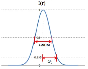
Where r is the beam radius along the radial axis or the optical axis, I(r) is the intensity of laser per unit area, ω0 is the beam waist, which is defined by the minimum beam radius where the intensity decreases to (=13.5%) of the peak intensity (as shown in Fig. 2-1), and P is the average power.

Full width half maximum (FWHM) is the common factor to describe the size of Gaussian distribution, and is the distance at the half of peak intensity as illustrating in Fig. 2-1. The FWHM can be simulated by PSF Lab software [23], it calculates the illumination point spread function (PSF) under various imaging conditions. The needed parameters for simulation are the NA of objective lens, the fill factor of the Gaussian illumination beam, the focus depth, the coverslip thickness, and the design and actual refractive index of the coverslip, immersion medium and resin respectively, as shown in Fig. 2-2 (a). PSF Lab only calculates the two dimensional slices of the illumination PSF; therefore, the xy, yz and xz plane can be chosen. After calculation, the FWHM in along the x, y and z axis can be obtained. The statistic result of PSF is showing in Fig. 2-2 (b).

Fig. 2-1 Intensity distribution of Gaussian beam and the definition of laser beam full width at half maximum and bean waist

(30)

(a) The illumination setup interface (b) The statistic result Fig. 2-2 The interface of PSF Lab software.

FWHM is the diameter at half of the maximum intensity and can be expressed as

𝐼 𝐼₀ =¹

2. (2-3)

And FWHM can be expressed as

2r = FWHM. (2-4)

The relationship between 𝜔₀ and FWHM by substituting Eq.(2-3) and Eq.(2-4) into Eq.(2-1), and the laser beam waist 𝜔₀ can be obtained as

ω₀ = √ ²

ln2 FWHM

2 ≅ 0.85 × FWHM. (2-5)

The TPP resolution is based on the size of voxel, which is important for the fabrication process. Fig. 2-3 (a) shows the top-view and side-view of the fabricated voxel, the lateral and longitudinal size can be informed by measuring the dimension of voxel. Fig. 2-3 (b) shows the spinning ellipsoid simulation a voxel, and the voxel width and voxel height are defined as 𝑣_𝑎 and 𝑣_𝑏.

(31)

(a) Top- and side-view of a voxel [24] (b) A spinning ellipsoid simulating a voxel [25]

Fig. 2-3 A voxel fabrication by TPP

Since the process of TPA depends on the square of the intensity [26], the voxel size can be predicted by setting I(r)² = 𝐼_𝑡ℎ²in Eq.(2-1), where 𝐼_𝑡ℎ is the threshold intensity of resin. Thus, the square of the threshold intensity can be expressed as,

2 0 4 2 2 0

2 

r

th I e

I



 . (2-6)

Therefore, the voxel width and voxel height can be expressed from Eq.(2-6) as,

th xy

a I

r 2lnI⁰

2 

   , (2-7)

th z

b I

r 2ln I⁰

2 

  

. (2-8)

Where 𝜔_𝑥𝑦 is the beam waist along the radial axis and 𝜔_𝑧 is the beam waist along the optical axis, both can be obtained from Eq.(2-5).

The voxel size are effected by the laser power, the threshold intensity of the resin and the beam waist from Eq.(2-7) and Eq.(2-8). By controlling the laser power to have it near the threshold power of resin, it is possible to create the high resolution products. On the other hand, for faster fabrication process or fabricating larger structures without concerning the resolution, the applied power can be two to three times the threshold power to fabricate higher aspect ratio voxel. These depend on the

(32)

need of quality of fabrication products.

2.2 The fabrication process of TPP

After applying the enough intensity of the laser, the liquid resin converts to solid phase at the focal position. The 3D structures can be obtained by moving the laser focal position with movable stage such as piezostage. A schematic diagram of TPP micro-fabrication is shown in Fig. 2-4.

Fig. 2-4 Schematic diagram of TPP micro-fabrication [25]

Layered manufacturing (LM) is a popular method for 3D printing. The conventional slicing method is the layer manufacturing (LM) method or also called the horizontal slicing method. The solid model is sliced layer by layer into 2-D closed contours in x-y plane, and each contour is divided into points as the scanning position.

User can decide particular parameters for slicing model, such as layer thickness and distance between points. The stage moves along these points and moves layer-by-layer until the last point of the last layer. With horizontal slicing method, the

(33)

method for Taipei 101 building.

Fig. 2-5 LM slicing method for Taipei 101 building

After the desired model is fabricated, the sample is immersed in the solution to move away the resin not polymerized. The fabrication result can be seen by SEM after metal coated. Fig. 2-6 shows the scheme of rinsing sequence. Each process would be illustrated in detail in the following sections

Fig. 2-6 The schematic of fabrication, immersion and the final desired product [26]

2.3 NTUMFS CAM system for TPP micro fabrication

National Taiwan University Micro Fabrication System (NTUMFS) is a computer aided manufacturing (CAM) system which is developed by CADLAB in ME department for TPP micro fabrication. The slicing parameters can be designed by user

(34)

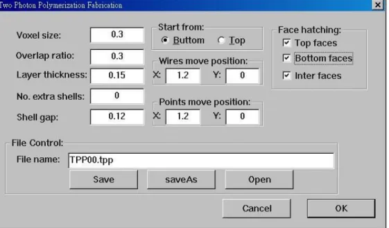
and the interface of the slicing program is shown in Fig. 2-7. The parameters in the interface including voxel size and overlap ratio, which can determine the voxel distance. Layer thickness, slicing sequence began from bottom to top or from top to bottom can be chosen. The slicing is based on the horizontal slicing method. To increase the shell stiffness of the structure, parameters of no. extra shells and shell gap can be used to create multipath. For fabricating solid structure instead of hollow one, the face hatching can be chosen.

Fig. 2-7 User interface of the slicing process

2.4 Experimental setup of TPP micro fabrication based on 3D piezostage

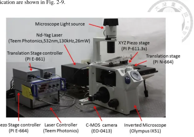
The schematic diagram of TPP micro fabrication system based on 3D piezostage is shown in Fig. 2-8. The TPP setup is based on a low-cost, double-frequency Nd:

YAG 532nm green light laser with average power 26mW and repetition rate of 130 kHz. The laser power is controlled by an attenuator, and then the laser is expanded

(35)

inverted microscope (OLYMPUS IX51), a dichroic mirror is used to reflect the laser into the objective. The laser is tightly focused into the resin by objective lens. Two different objective lenses, 100x-NA1.3 (Olympus UPLFLN100XO2) and 50x-NA0.8 (Olympus MPLFLN50X) are used. The coverslip is mounted on the 3D piezostage and has a thickness 170nm. The resin is laid on the top of coverslip for fabricating micro structures. A CMOS camera behind the dichroic mirror is used for monitoring fabrication process and optical adjustment.

Fig. 2-8 Schematic diagram of TPP micro fabrication system based on 3D piezostage The travel range of the piezostage is the maximum size of the fabricated structure.

The piezostage of the system is mounted on a two-axis stage providing 50x50 mm² for larger movement by hand. For the second one, the coverslip is fixed on the 3D piezostage (PI P-611.3) with travel range 100μm in each axis and can be exchange with another 3D piezostage (PI P-615) with travel range 350μm x 350μm x 250μm.

The piezostage is mounted on the computer-controlled translation stage providing 3cm x 3cm travel range. The experimental setups based on 3D piezostage for TPP

(36)

fabrication are shown in Fig. 2-9.

Fig. 2-9 Hardware setup with piezostage

2.5 Supercritical point drying process

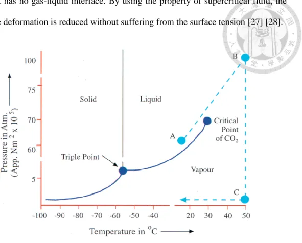
In the immersion process mention above, the resin not polymerized would be dissolved with solvent and the fabricated structure remains on the coverslip. However, after dissolving the resin not polymerized and put it in the air for nature drying, the surface tension of the solvent occurs while the solvent is evaporating. The surface tension causes the deformation and destruction of the structures. To avoid the influence of surface tension, the critical point drying (CPD) is adopted. CPD is a process to remove liquid in a controlled way. As shown in Fig. 2-10, when a substance changes from liquid to gas, it crosses the liquid-gas boundary on the phase diagram.

CPD provides a way to convert substance from liquid to vapor without crossing the liquid-vapor boundary, as the route passing A, B and C. Since the supercritical fluid

(37)

liquid, it has no gas-liquid interface. By using the property of supercritical fluid, the structure deformation is reduced without suffering from the surface tension [27] [28].

Fig. 2-10 Carbon dioxide pressure-temperature phase diagram

In this thesis, carbon dioxide (CO₂) is chosen as the supercritical fluid. The critical temperature and critical pressure of CO2 are 31.1°C and 7.38MPa. The manual critical point dryer (K850, Quorum) is adopted to do the drying process, shown in Fig. 2-11.

The procedure for operating the dryer is described as follows:

(1) Soak the sample into methyl isobutyl ketone(MIBK) for 8 minutes to soften resin which is not polymerized.

(2) Soak the sample into the acetone for 8 minutes to remove resin which is not polymerized.

(3) Cool down the empty chamber of CPD until temperature is below 5°C.

(4) Add acetone, which should be able to cover the sample, into chamber.

(5) Put the sample into chamber.

(6) Replace acetone in chamber with liquid CO₂ within 2 minutes.

(38)

(7) Heat the chamber until the temperature and pressure is beyond the critical point of CO2.

(8) Turn off heater and depressurize the chamber delicately.

The overall CPD process took around 1 hour. Fig. 2-12 shows the results of natural drying and critical point drying. The 3x3 micro spring array in Fig. 2-12(a) collapse and fall toward the center because of the surface tension. The springs shown in Fig.

2-12(b) stand completely with critical point drying. The difference proves that CPD is a necessary process for TPP micro-fabrication especially for structures with high aspect ratio.

Fig. 2-11 Manual critical point dryer K850

(39)

2.6 Scanning electronic microscope image

In order to obtain the dimension and the shape of the fabrication structures, the samples are imaged with SEM (either JEOL JSM-7000F or JEOL JSM-6390). The Auto Fine Coaters JEOL JFC-1600 is used to have the sample metal coated before taking the SEM picture. The material for coating is platinum and the sputtering time and electronic current are set to 60 seconds and 20mA respectively, the corresponding coating thickness is about 9nm.

(40)

Chapter 3 Large scale TPP system based on galvanometer scanner

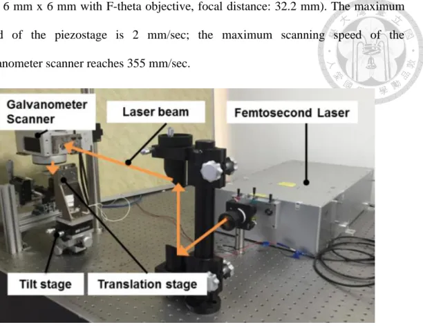
In this section, a large scale of TPP system integrating a femtosecond laser and galvanometer scanner has been established. By using f-theta lens and translational stage, the fabricating area can expend to 6 mm x 6 mm. Moreover, the maximum fabrication speed increased up to 175 times (355 mm/sec) compared with that of operated in the conventional piezostage (2 mm/sec). The new controlling software for galvanometer scanner and laser through scanner control board is also coded with C++.

It is highly expected that with the aid of rapid fabrication at this level could fully fit the demands of various repeatability tests and devices that are mandatory needed in cell mechanics and tissue engineering applications.

3.1 Hardware development of large scale TPP system

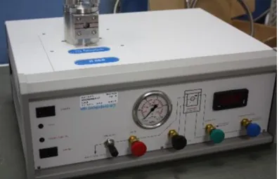
The large scale TPP system equipped with a high power femtosecond fiber laser (LightWire FF3000; repetition rate: 2MHz, operating wavelength: 515 nm, pulse energy > 2 µJ, beam quality: M² < 1.3). The maximum power of the laser is 4 W operated with 1030 nm wavelength. To make experiment much safer and convenient, laser was operated at double frequency. So that, invisible far infrared light becomes visible green light. To cooperate with the power, wavelength and repetition rate of laser, the matching initiator (1, 3, 5-Tris (2-(9-ethylcabazyl-3) ethylene) benzene) was chosen and mixed with OrmoComp® being able to be polymerized effectively and accurately. The experimental setup of the system is shown in Fig. 3-1. To improve

(41)

area: 6 mm x 6 mm with F-theta objective, focal distance: 32.2 mm). The maximum speed of the piezostage is 2 mm/sec; the maximum scanning speed of the galvanometer scanner reaches 355 mm/sec.

Fig. 3-1 The experimental setups of rapid TPP system

The schematic view of rapid TPP system is shown in Fig. 3-2. High power femtosecond laser beam passes through the 8x beam expander (Altechna 6-BE-Tx2-8, variable magnification: 2x to 8x), and into the scan head. The laser beam was steered by two scanning mirrors and then focused on the coverslip by an f-theta lens.

Meanwhile, a piezo-driven translation stage (PI E-861.1A1, high-resolution translation stage; maximum stroke: 30 mm, maximum load: 20 N) that manages the z-axis was implied to control the laser focusing point with precision up to 2 nm.

Those major devices of the TPP system as well as specifications are summarized in Table 3-1.

(42)

Fig. 3-2 The system set-up of two-photon polymerization system based on galvanometer scanner

Table 3-1 Major equipments and characteristics

Item Specifications

Femtosecond Laser

EKSPLA FF3000

Wave length: 1030nm/515nm Repetition rate: 2MHz

Output power: > 4W Pulse energy: > 2µJ

Galvanometer scanner

SCANLAB SCANcubeIII 14 Aperture: 14mm

Marking speed: 355mm/s Positioning speed: 2485 mm/s Scan angle: ±0.35 rad

Repeatability: < 2µrad

F-theta lens

Sill Optics S4LFT4031/121 Optical scan angle: ±7.6°

Working distance: 28.4mm Scan area: 6mm x 6mm

Translation stage

PI E-861.1A1

Maximum stroke: 30mm Sensor resolution: 0.5nm Maximum velocity: 10mm/s

(43)

The mirror galvanometer consists of a coil which is suspended by means of silken threads. When a direct current flows through the coil, the coil generates a magnetic field. This field acts against the permanent magnet and the coil twists. The basis of the operation is shown in Fig. 3-3. A small mirror is attached to the coil. The primary tasks of an X-Y scanner are to deflect a laser beam in the X-Y directions and to focus the beam onto the working plane. The light from a source enters the scan head through the input aperture and is first deflected in the Y direction by mirror 1 attached to galvanometer scanner 1. The beam then goes on to be deflected in the X direction by mirror 2 attached to galvanometer scanner 2. The resulting deflection angles can be precisely and high dynamically adjusted by controlling the positions of the galvanometer scanners so that the reflected light falls on a screen under precisely control.

Fig. 3-3 Beam deflection via galvanometer scanners

F-theta lenses are used in various applications on industrial material processing, drilling, welding and cutting. Standard lenses focus the laser beam on a spherical plain in contrast to an ideal flat or plane field. As shown in Fig. 3-4, The use of f-theta lens provides a plane focusing surface and almost constant spot size over the entire

(44)

XY plane or scan field. The position of the spot on the image plane is also directly proportional to the scan angle.

(a) Optic lens (b) F-theta lens

Fig. 3-4 The different between optic lenses and F-theta lenses

The scan head is operated via a SCANLAB RTC5 control board. Position signals are digitally transferred from the controller to the scan head. The scan head is calibrated in such a way that a scan angle of 0.408 rad in the negative axis direction with the bit-value "–503316" transmitted, the neutral position (null point) with the bit-value "0" transmitted, and a scan angle of 0.408 rad in the positive axis direction with the bit-value "+503316" transmitted. The image field size depends on the f-theta lens and the diameter of laser beam into the scan head. The maximum scanning area of the f-Theta objective is 6 mm x 6 mm. To get the positioning precision of galvo scanner, a grating with the length of 15000 bits is fabricated. The SEM image is shown as Fig. 3-5. The length measured with SEM is about 6.44mm. According to the measurement, the positioning precision is about 0.43µm corresponding to 1 bit.

(45)

Fig. 3-5 The maximum size of grating made with the rapid TPP system

3.2 Software design for large scale TPP system

The way to control scan head is similar to controlling piezostage. After slicing model with CAM system, NTUMFS mentioned in section 2.3, *.txt file of point data is exported as shown in Fig. 3.6. However, the unit of coordinates in *.txt file is micrometer for piezostage, but the unit for scan head is bit. According to the experiment mentioned before, the positioning precision is about 0.43µm corresponding to 1 bit. To fabricate product with correct dimension, the CAD model should be scaled with a scale factor 2.326 before slicing into point data.

Fig. 3-6 Part of scanning path data

(46)

The SCANLAB RTC® 5 control board and its related software are designed for controlling scan systems and lasers. To illustrate the principle of operation, Fig. 3-7 shows a simple laser marking sample. The image is made up of straight line segments (vectors) and arc segments. The RTC® 5 driver provides a set of jump, mark, arc and ellipse commands for laser processing along such segments. Each of these commands describes one vector or arc. Additional software commands are available for controlling the laser during the marking process.

Fig. 3-7 The laser marking sample of RTC5

As shown in Fig. 3-8, when executing a mark command, the laser is turned on and the scanner start moving to next position. If the position of each voxel is assigned continuously, the laser won’t be turned off and the focus point moved forward without staying at the coordinates assigned. Only if a jump command is executed, the laser is turned off. However, for TPP process, focus spot has to be located at the position for exposure time leading to necessary polymerization. To be able to control the system with correct TPP process, the set_laser_control (0x18) command is used to inverse the laser control signals for “Laser active” operation. After inversing the signals of laser control, the command used for laser processing is only jump command and the exposure time is decided with the jump delay shown in Fig. 3-8(b).

(47)

(a) Mark command (b) Jump command

Fig. 3-8 Scan head control timing during jump command and mark command For controlling piezo-driven translation stage managing the z-axis position, the scan head and stage movement is not synchronized due to the two controllers connected in parallel. While fabricating 3D structures, the incoordination causes the defect shown in Fig. 3-9. The reason is that the stage moves before the fabrication process of the recent layer has been done.

Fig. 3-9 Defect caused by incoordination between scanner and z-stage

(48)

To solve the problem, the C++ function Sleep() is added into program as shown in Fig.

3-10 for making the scanner and the stage be paused. In the process of fabrication shown in Fig. 3-11, the scanner controls the position of focus of first layer. After finishing the first layer, the scanner pauses 5000 ms until stage moves to the height of next layer. Then, the scanner starts to control the position of focus and meanwhile the stage pauses a moment according to the processing time of this layer. This design of program can avoid incoordination of system to happen.

Fig. 3-10 The code for delay between layer and layer

Fig. 3-11 Illustration of the code for delay between layer and layer

(49)

3.3 2D & 3D fabrication with large scale TPP system

To know the lateral and longitudinal resolution of the voxel fabricated with the f-theta lens, first of all, series of voxel are fabricated on the coverslip. OrmoComp®

with 1.2 wt% of photon-initiator is selected as material and four different exposure times (80, 60, 40, 20) are used. Fig. 3-12 shows the dimension of results with laser power 4W. It shows that lateral resolution is around 5μm. To know the longitudinal resolution of the voxel, suspended bridge method [13] is used as shown in Fig. 3-13.

The material is OrmoComp® with 1.2 wt% of photon-initiator. The minimum line with fabricated is 42.42μm with laser power 4W and exposure time 20ms. The aspect ratio is about 1:8.95 as results.

(a) Lateral diameter = 5.67μm with exposure time 80ms

Fig. 3-12 Voxel fabrication with OrmoComp®

(50)

Fig. 3-13 Line fabrication with suspended bridge method and OrmoComp®

In TPP fabrication system, the laser focus plane and the coverslip with resin may not be perfectly horizontal. The tilt correction is crucial for keeping the focus properly on the coverslip during fabrication process. The TPP system based on 3D piezostage calibrates the tilting effect of fabrication surface from the sliced data by a transferred matrix, which focal z position is continuously changed during the whole manufacturing process. The method using transferred matrix has an issue on axes synchronization. The process of the method is that using focuses of three points on the inclined coverslip to define the new coordinate system which should be the fabrication plane. Then the point date of each voxels on the horizontal plane is rotated to the new coordinate system. After correction, the z-coordinate of points at same layer become different while fabricating. However, the rapid TPP system is based on a galvanometric XY scanner incorporating Z-axis translation stage. The scanning speed of scanner is 355 mm/s and the velocity of stage is 10 mm/s. the difference of the speed makes the stage unable to catch the scanner and increase processing time greatly. To solve the problem, a tilt stage is applied to the rapid TPP system as show in Fig. 3-14.

(51)

Fig. 3-14 Illustration for the mechanism of the tilt stage

The procedure for tilt correction is described as follows: At the beginning, manual focusing is used to decide the z position of the three focuses by moving the translation stage with 1 µm. The three focuses are at corners of 6mm length square.

Then adjust the tilt stage manually until the three focuses are at same z position. The adjusting resolution of height is 1.54µm according to the resolution of the tilt stage which is 53 arcsec. The product of large area of 1 mm x 1 mm micro-grating with 20µm line pitch is shown in Fig. 3-15 (a), and the logo of National Taiwan University with 3mm diameter is shown in Fig. 3-15 (b). For Fig. 3-14, the voxel distance is 0.42μm, laser power is 1.2W, and the exposure time is 5ms. The fabrication time is 20mins for grating and 42mins for logo respectively.

(a) 51 x 51 grating with 20 µm line pitch (b) NTU Logo with 3mm diameter Fig. 3-15 SEM image of 51 x 51 grating and NTU Logo

For 3D fabrication, to be able to fabricate the structures with high aspect ratio, OrmoComp® was injected into a tank made with restickable tape (Scotch®

(52)

Restickable Strips) with 5 mm height on the coverslip with 160μm thickness to make the resin level can cover the structures. The setup is shown in Fig. 3-16. Structures with high aspect ratio can be fabricated with the setup as shown in Fig. 3-17. The slicing parameters are set as following: voxel distance = 1.72μm, layer thickness = 43μm, offset distance = 1.72μm, number of extra shells = 2. The sizes of the tubes are 116.67μm inner diameter, 140.01μm outer diameter and 1mm height. The processing time is about 20mins.

Fig. 3-16 OrmoComp® setup for higher structures bounded by the tape on coverslip

(a) Top view (b) Side view

Fig. 3-17 tube structures fabricated with 116.67μm inner diameter, 140.01μm outer

(53)

While fabricating large-area structure on the coverslip, the structure is easily separated from coverslip as shown in Fig. 3-18 after removing resin not polymerized.

The most possible reason is the force from shrinkage. When the polymerized volume becomes larger, the shrinkage force also becomes larger. Therefore, the adhesion cannot sustain the strain that comes from shrinkage, and the structure warps. One of solution is eliminating shrinkage of structure by adding anchor support [35]. The structure with an array of 16 μm diameter anchors is fabricated as Fig. 3-16 (b) shown without distortion.

(a) Without anchors structures (2000µm x 200µm x 200µm)

(b) With anchors structures (2000µm x 400µm x 200µm)

Fig. 3-18 SEM image of large scale structures

Another solution is enhancing the adhesion force with adding grating structure between coverslip and structure as shown in Fig. 3-17. However, the two solutions change the configuration of the structure. For improving the binding, a commercial product, adhesion promoter, is suggested to be primed on the substrate. In order to ensure good adhesion of the polymers to substrates such as glass, silicon or plastics, the surface of the substrates has to be primed with an adhesion promoter

(54)

(a) Top view (b) Side view Fig. 3-19 The SEM image of large scale structures with grating base

(55)

Chapter 4 Design and fabrication of substrates for cell migrating with TPP

In this section, TPP technology is used to nanofabricate substrates with various curvature and surface roughness for investigating the influence of surface topology on cellular behaviors of MG63 human osteosarcoma cells. By applying the full width half maximum of focused laser intensity as a necessity of two photon absorption, the point spread function (PSF) was applied to simulate the size of polymerized voxels.

With the calculation of route design, voxel position control, and the verification from experimental results of confocal analysis, the calibration of surface roughness and voxel distance is proposed for studies on cell migration.

4.1 Experimental setup for fabrication of substrates

To investigate the influence of surface topology on cellular behavior of MG63 human osteosarcoma cells, TPP technology is used to nanofabricate substrates with various curvatures. Aiming to fabricate the structures with the size over 200μm, the PI P-615 piezostage is selected. Hoi tested the mechanical response of the piezostage with the fabrication path of Fresnel zone plate (FZP) [29]. The oscilloscope signal of the piezo-stages PI P-611 and PI P-615 are in the shape of FZP as shown in Fig. 4-1 with the same exposure time of 5ms. It can be seen from Fig. 4-1 that by comparing the shape of FZP, the shape fabricated with PI P-615 becomes ellipse.

(56)

(a) PI P-611 (b) PI P-615

Fig. 4-1 Mechanical response between PI P-611 and P-615 with exposure time 5ms [29]

To quantify the form error of structures fabricated with P-615 piezostage, the various sizes of gratings were designed and fabricated. While fabricating a 280μm x 280μm grating with pith of 20μm as shown in Fig. 4-2, the error of length along x-axis is 3.32%, the error of length along y-axis is -7.32%, and the error of angle is 2.2°. The measured error of length along two axes with different size in Fig. 4-2 is plotted in Fig. 4-3.

Fig. 4-2 The CAD model and SEM image of the testing grating

(57)

Fig. 4-3 Diagram of length error versus various grating size.

From the above results, it can be observed that the error of length along x axis increases as the grating size increases and the error of length along y axis decreases as the grating size increases. According to the fitting lines shown in Fig. 4-3, the C++

program was developed with Visual Studio 2015 to calibrate the coordination of each voxel before fabrication. The difference with and without calibration can be observed from the SEM images of the two name cards in Fig. 4-4. After applying calibration, the form error is improved as shown in Fig. 4-4 (b). It is indicated that the form error of PI P-615 have been solved.

(a) Without calibration (b) With calibration

Fig. 4-4 Form error calibration of PI P-615 piezostage with size of 270 µm x 180µm name cards

(58)

For fabricating structures effectively with larger voxels, the 50x-NA0.8 objective lens (Olympus, MPlanFLN) is used. However, the voxel shape is strongly related to the optical point-spread function (PSF). The PSF is determined by the NA of the focusing optics and by aberration. Spherical aberration happens when focused light passes interfaces of materials with different refractive indices. It results in a blurring of the optical PSF especially in the vertical direction. The amount of spherical aberration depends on the refractive index mismatch, the NA, and the penetration depth d of the focus into the material as shown in Fig. 4-5. During fabrication process, the penetration depth d increases, withd = d^′+ ∆, d^′ is the thickness of coverslip (170 µm), and ∆ is the z coordinate of each voxel.

Due to spherical aberration, the PSF is strongly elongated with additional maxima occurring deeper in the material with distances and intensities that are increasing with increasing d. The widths of FWHM are increasing in the x and y direction from a value of 0.377μm (∆ = 0µm) to 0.483μm (∆ = 40µm)and in the z direction from 2.160μm (∆ = 0µm) to 5.179μm (∆ = 40µm), which shows that spherical aberrations mainly affect the axial extension of the PSF.

Fig. 4-5 Exposure strategy and spherical aberration due to refraction at interfaces of

(59)

inverted as Fig. 4-6 shown. Because the laser beam passes only through the resin without through the coverslip, spherical aberration, arising from refractive index mismatch at interfaces, happens only once. The thickness of resin usually is about 100µm less than the coverslip. The penetration depth is less than the one without inverse. The less perpetration depth laser passes, the less voxel is out of shape. So that, with the exposure strategy that resin put below coverslip, the better shape of structure and the higher structure can be fabricated.

Fig. 4-6 Schematic view of the different exposure strategies

As Fig. 4-7 shown, Taipei 101, a complicated structure with high aspect ratio, is used to demonstrate the different between two exposure strategies. The CAD model of Taipei 101, the width and height is 40 µm and 193 µm respectively. For using the exposure strategy, the objective lens has to be 0.8NA. The slicing parameters are set as following: voxel distance = 0.5µm, layer distance = 1.0µm, number of extra shell = 1. To enhance the strength of the 101 building, the structure was fabricated with solid model rather than shell model shown in Fig. 4-8 (a) and (b). The laser power is 5mW and exposure time is 3ms. It can be observed that the Taipei 101 fabricated with resin put below coverslip has much more details and the height can be the same with the thickness of the resin. Compare to the previous work, the Taipei 101 fabricating with exposure strategy that resin above coverslip has less details and limit on the height as

(60)

Fig. 4-8 (c) and (d) showed [28]. In this case, using lower NA objective lens and with exposure strategy that resin below coverslip are suitable for fabricating the structures with height over 20 µm scale.

Fig. 4-7 CAD model of Taipei 101 with size 193 µm x 40 µm x 40 µm.

(a) Top view with below resin (b) 45 degree view with below resin

(61)

4.2 Fabrication strategy of substrates with different curvature on surface

To investigate the influence of surface topology on cellular behaviors of human osteosarcoma cells named MG63, the structure with certain curvature was designed and the parameters are shown in Fig. 4-9. The model is separated into three parts, as shown in Fig. 4-10. The slicing strategy for surface part was changed from horizontal to vertical slicing to make top smoother. However, the fabrication sequence Fig.

4-11(a) shows that the surface of structure fabricated with vertical slicing method is not continuous. There are four gaps on the surface. After checking the sequence of scanning paths, it can be found that the defect is caused by dislocation of scanning path. From the layered manufacturing concept, a solid model of the structure is sliced vertically into 2D contours as fabricating process, and each path is divided into scanning points. After slicing models into scanning paths with NTUMFS developed by commercial CAD software AutoCAD with built-in AutoLISP program, the AutoLISP program exports point data with selecting scanning paths. Under the condition of fabricating structures with 10~50 µm scale, the numbers of selected layers is below 200. However, while fabricate structures with size over 150µm, the number of entities in the selection set is over about 200. As Fig. 4-12 shown, the sequence of entities in a selection set becomes noncontinuous. In order to solve this problem, the AutoLISP program was modified and be able to sort by vertex X or Y defined by AutoCAD. The product fabricated with modified program is shown as Fig.

4-11 (b). The gaps caused by discontinuous fabricating sequence disappear after sorting the whole entities generated with horizontal slicing method.

(62)

Fig. 4-9 Design parameters of curvature substrate

Fig. 4-10 Slicing strategies of different patrs of curvature substrate

(a) Without sorting (b) With sorting

Fig. 4-11 Curvature substrates fabricated with TPP

(63)

Fig. 4-12 Top view of fabricating sequence with the unsorting scanning paths (the arrow in structure means the scanning sequence of each slicing layer)

To increase the number of MG63 cells seeded on the substrates, another type of substrate was designed with different curvature on surface as shown in Fig. 4-13. In order to observe whether MG63 cells migrate through the scanning direction and have enough samples to quantify the migrating velocity of the cells, a total twelve substrates, two identical substrates with two control variables (two perpendicular scanning direction and three different curvature surfaces), should be fabricated onto a same coverslip. However, for the long time fabrication, the quality of resin is changed.

In the view of this, the substrates should be fabricated with shell model rather than solid model. According to the previous work, the CAD models were separate into two parts for mixed slicing method as shown in Fig. 4-14 (a). The slicing parameters are set as following: voxel distance = 0.5μm, layer distance = 0.8μm, number of extra shells = 5, offset distance of shells = 0.5μm. The laser power is 6mW, exposure time is 3ms, and the processing time is 55 minutes for Fig. 4-14 (b). It is obvious that the substrate collapses due to the shells overwhelm resin without polymerization so that the resin leaked from the fragile part of substrate.