Testing the Equality of two Survival Functions with Doubly
Truncated Data
Yunchan Chi1
Department of Statistics, National Cheng-Kung University, Tainan, Taiwan R.O. C.1
SUMMARY. Recently, several algorithms, such as Turnbull (1976) and Efron and Petrosian (1999), have been derived from the likelihood function to estimate the survival function based on doubly truncated data. However, the nonparametric methods for comparing the two survival functions have not yet been developed. Therefore, this paper proposes two test statistics to test the equality of two survival functions for doubly truncated data. One is based on the integrated weighted difference between the two estimated survival functions, while the other is similar in form to the usual weighted logrank test. The implementation of these methods to the lifetime data of Taiwan’sbuildings is presented and the comparative results from a simulation study are discussed.
KEY WORDS: Doubly truncated data; Integrated weighted difference; Logrank test; Self-consistent estimator; Survival function
1. Introduction
Doubly truncated data arise frequently from some sampling schemes, such as cross-sectional sampling (Wang, 1991), and retrospective sampling (Bilker and Wang, 1996), in several areas including economics, astronomy, industry and medicine.Forexample,theTaiwan’sbuilding lifetimesdatasetcollected by the Department of Architecture at the National Cheng Kung University to investigate the life span of all kinds of buildings in Taiwan area is doubly truncated. Since the administration of building was not computerized until 1990s, a large amount of data before 1981 was not included in computer databases. Due to this limitation, in conducting the investigation, the researchers sampled the buildings from the Taiwan deconstruction permits database from 1981 to 2001.
Then the date of building construction was retrospectively ascertained for all cases in which the deconstruction permits were issued between January 1981 and December 2001. Consequently, for those buildings which were demolished before 1981, and those after 2001 cannot be included in the database, or were doubly truncated. This implies that buildings with much shorter or much longer lifetimes are hardly observed by this sampling scheme and failure to account for doubly truncation can lead to biased inference. Turnbull (1976), Alioum and Commenges (1996), Bilker and Wang (1996), and Efron and Petrosian (1999), among others are devoted to develop statistical methods to accommodate doubly truncation.
To compare the survival functions based on doubly truncated data, Bilker and Wang (1996) suggested a semiparametric version of the Mann-Whitney test by assuming the distribution of truncation times (for instance, the time from construction to 1981 or to 2001) is known or can be estimated parametrically.
Alioum and Commenges (1996) developed the Wald test for testing zero
regression coefficient in a proportional hazards model. Although a semiparametric test may have greater efficiency, it is sensitive to model misspecification. Therefore, this paper proposes two nonparametric test statistics when the data are measured on a discrete scale. One is based on the integrated weighted difference between two estimated survival functions (Turnbull, 1976;
Efron and Petrosian (1999)), while the other is a modification of the usual weighted logrank test.
The rest of this paper is organized as follows. Section 2 gives the necessary notation and technical terms for understanding the impact of doubly truncation.
The self-consistent estimate of conditional survival function given by Efron and Petrosian is reviewed in Section 3, and its variance estimator is derived from the likelihood function in the same section. The proposed tests are developed in Section 4. The applications of these tests to the lifetime data of Taiwan’s buildings are demonstrated in Section 5. Simulation comparisons between the proposed tests and the usual weighted logrank test are discussed in Section 6.
Finally, some concluding remarks are given in the last section.
2. Preliminary
The purpose of this section is to formally define the notation for doubly truncated data and to review technical terms to better understand the effect of truncation. According to the Taiwan’s building lifetime data, X denotes the construction date and Y denotes the lifetime. Hence, the date of building deconstruction is X+Y and only the buildings with X+Y between A and B were included in the data set. Note that AX = U and BX = V are often referred to as left and right truncation times, respectively. In more general setting, doubly truncated data arise when one can only observe Y if U Y V . These data are
denoted by (Uk,Yk,Vk)=(uk, yk, vk), for k = 1,2,…,n.
Next, several technical terms have to be used to help understand the impact of truncation. If the lifetime Y and the truncation time X are independent, then the joint probability density distribution (p.d.f.) of Y and X in the region
B Y X
A is
) (
] [
) ( ) ) (
,
( P A X Y B
B y x A I x g y x f
y
k
,
where f(y) and g(x) are the p.d.f. of Y and X, respectively, I[.] is an indicator, and P(AX Y B) denotes the probability that X+Y lies between A and B.
Moreover, the marginal distribution of X, given AX Y B and X = x, is
) (
] [
) ( ) (
B Y X A P
dy B y x A I x g y f
v
u
,
Thus the conditional distribution of Y given AX Y Band X = x is
) (
] [
) ( ) (
) (
] [
) ( ) (
B Y X A P dy B y x A I x g y f
B Y X A P B y x A I x g y f
v
u
,and the above expression can be simplified as
) ( ) (
) ) (
*(
u F v F
y y f
f , for uyv
where F(y) is the distribution function of Y. Furthermore, for given B
Y X
A and X = x, the conditional survival function of Y is )
| ( )
*(
v Y u y Y P y
S
) ( ) (
) ( ) (
v S u S
v S y S
(1)
However, the survival functionS(y)P(Yy)is non-identifiable (Tsai and Zhang (1995)), only S*() can be estimated uniquely. Therefore, under doubly truncation one can only estimate the conditional survival function of Y in the region (l, r)
)
*( y
S ( ) ( )
) ( ) (
r S l S
r S y S
.
In practice l and r are often chosen to be the minimum values of the observed left truncation times and the maximum values of observed right truncation times, namely lmin{uk,i1, , n} and rmax{vk,i1, , n}, respectively.
Since the goal of this paper is to provide nonparametric methods for testing the equality of two survival functions, let (uik, yik, vik) denote the doubly truncated data collected from the ith sample, for i=1, 2, and k1, 2, , ni. Furthermore, let 1(1) 1(2) 1( )
m1
y y
y and 2(1) 2(2) 2( )
m2
y y
y denote
the ordered distinct lifetimes of the first and second samples, respectively, and let y(1) y(2) y(m) be the distinct ordered observed lifetimes in combined samples. Because the survival functions of Yik are not identifiable under truncation, one can only estimate the conditional survival function of the ith group in the region (li,ri), where in practice l andi r are often chosen to bei the minimum values of observed left truncation times and the maximum values of observed right truncation times, namely li min{uik,k1, , ni} and
} , , 1 ,
max{ ik i
i v k n
r , respectively. However, a fair comparison between the two conditional survival functions should be in the same region (1,2) based on the doubly truncated data. When the truncation patterns of the two groups are unknown, and1 are chosen to be2 max(y1(1),y2(1)) and
) , min( 1( ) 2( )
2
1 m
m y
y ; respectively, in practice. Hence, the null and alternative hypotheses tested in this paper are
) ( ) (
: 1* 2*
0 S y S y
H y(1,2)
) ( ) (
:S1* y S2* y
Ha for some y(1,2)
Note that if H0 is rejected, one can conclude that the survival functions of the two groups are different.
3. Self-consistent estimates of conditional survival function
One nonparametric test proposed here is based on the weighted difference in survival estimates, thus the algorithms for estimating conditional survival function are reviewed in this section. The conditional survival functions of the two groups can be estimated either by a self-consistent algorithm proposed by Turnbull (1976) or a self-consistent algorithm derived directly from the likelihood function based on doubly truncated data, which is equivalent to an algorithm developed by Efron and Petrosian (1999). These self-consistent algorithms all produce the same estimates of the conditional survival function, but each serve a different purpose. For example, the latter two algorithms lead to different types of test statistics for testing the equality of two conditional survival functions and these two algorithms are reviewed in the following.
To simplify the notation, the subscript indicating group is dropped for the following derivation. Based on a random sample of doubly-truncated data
) , ,
(Uk Yk Vk =(uk,yk,vk), for k 1, 2, , n, the likelihood function is
n
k k k
k
u F v F
y L f
1 ( ) ( )
)
( .
Let Pj be the probability that an event occurring at y( j), and let Jkj= 1 for )
,
) (
(j uk vk
y and Jkj= 0, otherwise. Then the denominator in the likelihood
function can be expressed as
m
j j kj k
k F u J P
v F
1
) ( )
( and denoted by F . Ink
addition, let dj=
n
k
j
k y
y I
1
) ( ]
[ count the number of failure events at y( j). Thus, the likelihood function based on the doubly truncated data becomes
L
n k
k m
j
d j
F P j
1 1
) (
. (2)
A self-consistent estimator for Pj, j = 1,2,…,m, can be derived directly from this likelihood function, and the resulting self-consistent equation is given by
n
k k
kj j j
J F P d
1
1 .
As a result, the self-consistent estimator of the conditional survival function for
the ith group is
m
j k
ik j
i y P
Sˆ( ) ˆ
)
( , where Pˆ is an estimate of the probabilityij that an event occurring at y( j) for the ith group. Accordingly, the covariance of
conditional survival probabilities evaluated at y( j) and y(k) is
ˆ( ), ˆ( )
ˆvSi y(j) Si y(k) o
C
m
j l
m
k h
ih il P P v o
Cˆ(ˆ, ˆ),
where Coˆv(Pˆij,Pˆih) can be obtained from Fisher information matrix based on the likelihood function (2) and given in Appendix A.
Efron and Petrosian (1999) criticized the above self-consistent algorithm for its slow convergence rate. Consequently, they proposed an algorithm on a basis of the number of subjects at risk and proved that these two algorithms essentially produce the same estimates of conditional survival function.
Moreover, their algorithm provides an intuitive explanation on how to account for the truncation effect. In addition, the number of subjects at risk at time y( j) can be estimated from their algorithm which is briefly reviewed as follows. The survival function can be expressed as S(y( j))=
j l
h )]l
1 log(
exp[ , where hj is
the hazard evaluated at timey( j). Based on the likelihood function in (2), Efron
and Petrosian suggested estimating S(y( j)) by estimating hj iteratively in terms of
n
k k
k kj j
j j
F J G N
h d
1 ˆ
ˆ ˆ,
j = 1,2,…,m, where [ ( ) ]
1
k j k n
k
j I u y y
N
counts the number of subjects at risk in the observable range at time y( j),
m
j j kj
k J P
F
1
ˆ
ˆ estimates the
probability that a failure event may occur in the range (uk,vk) , and
m
j
j j k
k I v y P
G
1
)
( ]ˆ
ˆ [ estimates the probability that a failure event may occur in the range (vk,), which is not observable due to right truncation. Thus, the
term
n
k k
k kj F J G
1 ˆ
ˆ
is used to estimate the number of subjects that may at risk at
time y( j) in the range we are not able to observe. Hence,
n
k k
k kj
j F
J G N
1 ˆ
ˆ can
serve as an estimate of the number of subjects at risk at time y( j), when there is no truncation. Consequently, the log-rank type test statistic based on the risk set will be examined in the next section.
4.
The proposed methods
Both Bilker and Wang (1996) and Alioum and Commenges (1996) developed semi-parametric tests to compare the two survival functions.
However, semi-parametric tests often suffer from substantial power loss under model misspecification. Therefore, two nonparametric test statistics in a discrete time framework are proposed in this section. A test based on the integrated weighted difference between the two estimated conditional survival functions is given in subsection 4.1, whereas a modification of weighted logrank test is derived in subsection 4.2.
4.1 Integrated Weighted Difference Test
To compare the conditional survival functions of the two groups, it is natural to examine the difference between the two estimated conditional survival functions;
) ˆ(
) ( j i y
S . Tsai and Zhang (1995) have developed the asymptotic normality of this estimator; however, its asymptotic variance is implicit and complicated.
Moreover, it is not easy to establish the asymptotic distribution of the difference between two estimated conditional survival functions in a continuous time framework. Thus, following the concept of Pepe and Fleming (1989) and Petroni and Wolfe (1994), a test statistic based on the integrated difference between the two estimated conditional survival functions is proposed here when data are measured on a discrete scale with a finite number of possible event times.
It should be recalled that the conditional survival function of the ith group;
) ( ( )
* j
i y
S , is estimated separately in the region (li,ri) , however, a fair comparison between the two conditional survival functions should be in the same observable region (1,2). In practice, when the truncation patterns of the
two groups are unknown, and1 are chosen to be2 max(y1(1),y2(1)) and )
, min( 1( ) 2( )
2
1 m
m y
y ; respectively. As a result, the estimated conditional survival functions have to be truncated in this region, and denoted by
) ˆ( ) ˆ(
) ˆ( ) ˆ( )
~ (
2 1
2 )
( )
(
i i
i j i j
i S S
S y y S
S
.
Then we propose the following test statistic
j y
j j
j
j
y S y S y w
D
( ) 2
1
))
~ ( )
~ ( )(
( ( ) 1 ( ) 2 ( )
,
where j y(j) y(j1), and w( y) can be an arbitrary or a data-dependent weight function chosen to be more sensitive to detect certain alternatives. In practice, the weight function can be identified from the plot of two estimated conditional survival functions truncated in the same region. For example,
) ( y
w =y is appropriate for detecting late survival difference, while w( y)= 1 is appropriate for detecting constant difference between two conditional survival functions across time. Note that when w( y)= 1, the statistic D is actually the difference between the two mean survival times,
m
j
j j m
j
j
j S y
y S
1
) ( 2 1
) (
1 ~ ( )
)
~(
, The variance of D is estimated by
D r aV ˆ =
2
1
) ( )
( )
( ) (
2 ) (
1 1 ( ) 2
))
~( ),
~( ˆ( ) ( ) (
i
q j
y y
q i j i q
j
j q
y S y S v o C y w y w
,
where the computation formula of ~( )) ),
~(
ˆv(Si y(j) Si y(q) o
C is given in
Appendix A. Let IWD = D / Vaˆ Dr( ) , using the idea of maximum likelihood, it can be shown that, under the null hypothesis
) ( ) (
: 1* 2*
0 S y S y
H for y(1,2), the asymptotic distribution of IWD is standard normal. Hence, the IWD test rejects the null hypothesis if
|IWD|z/2, where z is the upper percentile of a standard normal distribution.
4.2 Modified Weighted Logrank Test
In the survival analysis, weighted logrank test is the most frequently applied test statistic for testing the equality of two survival functions when the data are subject to right censoring. The most easily understood form of weighted logrank test is based on the sum of weighted differences between observed and expected number of failure events; namely
U =
m
j
j j
j d e
w
1
1
1 )
( ,
where w are weights chosen to let U be more sensitive to detect certainj alternatives, dij is the number of failure events of the ith sample at time y( j), e1j
= n1j(d1j+d2j)/(n1j+n2j) is the number of expected failure events occurring at time y( j) of the first sample with nij being the number of subjects at risk at time
)
y( j of the ith sample, for i = 1, 2, and j = 1,2,…,m. Moreover, a consistent estimate of the variance of U is given by
Ur a
V ˆ =
m
j j j j j
j j j j j j j j
j n n n n
n n d d n n d w d
1 1 2
2 2 1
2 1 2 1 2 1 2 2 1
) 1 (
) (
) )(
( ,
Let WLR = U / VaˆUr( ), it can be shown that, under the null hypothesis H0: )
1(t
S =S2(t), the asymptotic distribution of WLR is standard normal.
It is worth noticing that the essential ingredient of weighted logrank test is the difference between the observed and expected number of failure events. To compute
the expected number of failure events, the risk set has to be defined properly. Once this set can be defined properly, one can directly apply the weighted logrank test to a variety of data types. For example, Lynden-Bell (1971) suggested a delayed-entry method to define the risk set and hence the number of subjects at risk when the data are subject to left truncation. As a result, the weighed logrank test can be applied.
However, there is no way to count directly the number of subjects in the risk set for right-truncated data. Consequently, Lagakos et al. (1988) proposed a weighted logrank test based on reverse time.
Nevertheless, according to the self-consistent algorithm proposed by Efron and Petrosian, it is natural to estimate the number of subjects at risk at y( j) of the ith sample for doubly truncated data by nˆij =
ni
k ik
ik ikj
ij F
J G N
1 ˆ
ˆ
, where ]
[ ( )
1
ik j ik n
k
ij I u y y
N
i
counts the number of subjects at risk in the observable range at time y( j),
mi
j
ij ikj
ik J P
F
1
ˆ
ˆ estimates the probability that a failure event may occur in the observable range (uik,vik) , and
mi
j
ij j ik
ik I v y P
G
1
)
( ]ˆ
ˆ [
estimates the probability that a failure event may occur in the range (vik,), which is not observable due to the right truncation. Thus, the term
ni
k ik
ik ikj F J G
1 ˆ
ˆ
is used to estimate the number of subjects that may be at risk at time y( j) in the range we are not able to observe. Therefore, nˆij is an estimate of the number of subjects at risk at time y( j) for the ith sample when there is no truncation. However, as mentioned in subsection 4.1, the two groups have to be compared in the same observable range
) ,
(1 2 . Thus, it is necessary to replace Gˆik and Fˆik by
2 ) ( 1
]~
~ [
) (
yj
ij j ik
ik I v y P
G and
m
y
ij ikj ik
j
P J F
2 ) ( 1
~
~
, respectively, where P~ij
= )
~ ( )
~ (
) 1 ( )
(j i j
i y S y
S . In addition, the number of subjects at risk is estimated by
n~ij=
ni
k ik
ik ikj
ij F
J G N
1
~
~
. Thus, one naive extension of weighted logrank test is to replace nij by n~ij in both U and V ˆar
U . The resulting test statistic is denoted by WLR_E. As demonstrated in the simulation, however, the normal approximation of WLR_E is incorrect due to variance underestimation.It’s not easy to find the variance of U when nij are estimated from a self-consistent algorithm. By some algebra, however, it is easy to express the usual weighted logrank statistic U as
m
j j
j j j j j
j j
j n
d n d n n
n w n
1 2
2
1 1
2 1
2
1 ,
Immediately, one recognizes that the terms inside the bracket; namely
ij ij
ij d n
h / , are the hazard estimates based on the number of subjects at risk at time y( j) of the ith sample. This expression enables us to construct a test similar in form to the weighted logrank test. For example, one can replace the above hazard estimates by h~ ij dij/n~ij. Hence, we propose
) 2 ( ) ( 1
2 1 2 1
2
1 ~ ~
~
~
~
~
yj
j j j j
j j
j h h
n n
n
n ,
as a test statistic, where can be an arbitrary or a data-dependent weightj function chosen to be more sensitive to detect certain alternatives. To simplify variance formula, let w~j=jn~1jn~2j/n~1j ~n2j, and the test statistic proposed here is based on
2 ) ( 1
~ ) (~
~
2 1
yj
j j
j h h
w
U ,
Since sample 1 is independent of sample 2, the variance of U can be expressed as
) (U
Var
j
y jh w Var
j
1
~ ~
2 ) (
1
j
y jh w Var
j
2
~ ~
2 ) (
1
,
and is simplified as
2
1 1 ( ) 2 1 ( ) 2
~ )
~ ,
~ (
~
i y y
iq ij q
j
j q
h h Cov w w
.
Since h~ij
is not directly estimated from self-consistent algorithm or the likelihood function, the observed Fisher information matrix cannot be used to estimate the covariance between h~ij
and h~iq
. However, with the help of this equivalent relationship Si(y( j)) =
j l
h )]il
1 log(
exp[ , the
variance of U can be derived in a discrete time framework. The
formula of ~ )
~, (hij hiq
Cov is given in Appendix B. Let WLR_M = U / Vaˆ Ur( , according to likelihood theory, it can be shown that, under)
the null hypothesis H0:S1*(y)S2*(y) for y(1,2) , the asymptotic distribution of WLR_M is a standard normal. One can reject the null hypothesis, if |WLR_M|z/2, where z is the upper percentile of a standard normal distribution.
5.
Example
In this section, the proposed methods are illustrated through Taiwan’s building lifetime data set. The concept of green building has been
developed to save energy and protect environment, such as increasing the efficiency in using energy, water and materials and reducing building impacts on human health and the environment, through better design, construction, operation, maintenance, and removal –the complete life cycle. Many rating systems have been developed for evaluating the complete life cycle of new buildings, including LEED (Leadership in Energy and Environmental Design). One of the key issue in life-cycle analysis is the estimate of building lifetime and hence the estimate of overall energy use and material consumption. To estimate the energy cost, the life cycle analysis of the existing buildings is also desirable.
Therefore, the Department of Architecture at National Cheng Kung University collected the life span of all kinds of buildings in Taiwan area.
Since the administration of building was not computerized until 1990s, a large amount of data before 1981 has not been included in the computer databases. Due to this limitation, in conducting the investigation, the Department of Architecture sampled the buildings from the Taiwan deconstruction permits database from 1981 to 2001. Then the date of building construction was retrospectively ascertained for all cases in which the deconstruction permits were issued between January 1981 and December 2001. Consequently, for those buildings which were demolished before 1981, and those after 2001 cannot be included in database, or doubly truncated. This data set consists of the lifetimes of buildings with various construction materials from four metropolitan areas of Taiwan.
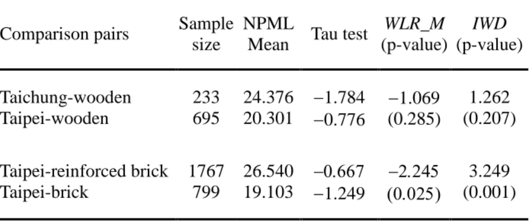
Now, the test statistics proposed in the previous section are applied to compare the lifetime distributions of wooden buildings in Taipei and
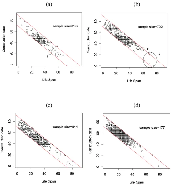
Taichung areas. Further, the lifetime distributions of reinforced brick and brick buildings in Taipei area conditional on a common observable range are compared. Since the proposed tests are based on the estimates from the self-consistent algorithms which are all derived from the conditional likelihood functions based on the assumption of independence of truncation times and survival times, it is desirable to examine the satisfaction of this assumption. The tau statistic modified by Efron and Petrosian (1999) are used to test this assumption and the results are listed in Table 1. Based on a two-sided test and at 0.05 significant level, the independence of truncation and survival times is satisfied. Figure 1 displays the scatter plots of building lifetimes versus construction dates from Taipei-wooden, Taipei-brick, Taipei-reinforced brick and Taichung- wooden. The self-consistent algorithms reviewed in Section 3 are used to obtain the conditional survival function estimates and mean lifetimes in the observable range. In practice, these algorithms work only when all data points are connected (Vardi, 1985). We define the concepts of connected sets of points in terms of comparable pairs of points. Two points y1 and y2 are said to be comparable if y1(u2,v2) and
) , ( 1 1
2 u v
y , and hence y1 and y2 are connected. In addition, if y1 and y2 are not comparable buty and2 y are comparable and3 y3 and y1 are comparable then y1 and y2 are also said to be indirectly comparable and hence connected. Consequently, y ,1 y and2 y3 all together can estimate the conditional survival function. For example, the panel (a) in Figure 1 shows that the points in both circle A and circle B are comparable. In addition, A is not comparable with B but both of them are comparable with the points in circle C. As a result, A and B are connected.
If a point is not comparable or indirectly comparable with any other points, then this point will be disconnected with the rest of data points.
For example, the point in circle B is not comparable with any points in circles A and C in Figure 1 panel (b). In other words, the points in A and B are not comparable with the rest of the points. Thus these 7 points have to be deleted to perform the self-consistent algorithm.
(Figure 1 is about here)
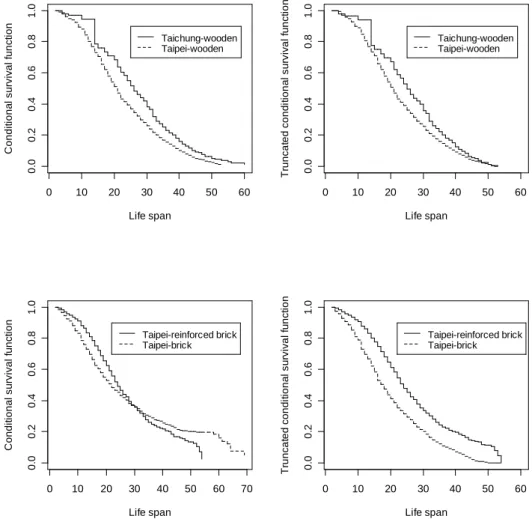
The estimated conditional survival functions and truncated estimated conditional survival functions of these lifetimes are plotted in Figure 2. The plot of Taipei reinforced brisk versus brick suggests that constant weight is appropriate for both the LR_M and IWD tests. Note that the WLR_M test with constant weight is referred to as modified logrank test (LR_M). Whereas, the constant weight is less appropriate for the comparison between Taipei wooden and Taichung wooden, but the departure from constant weight is small. The comparison result is listed in Table 1. The estimated conditional survival function of lifetimes of wooden buildings in Taichung is slightly higher than that in Taipei since Taipei was developed earlier than Taichung. However, based on one-sided test, the difference is not significant. On the other hand, the survival function of the lifetimes of reinforced buildings is higher than that in brick buildings thanks to reinforced material which is more durable than brick.
(Figure 2 and Table 1 are about here)
6. Simulation Results
To investigate the performance of the proposed methods in the comparison between two survival functions conditional on the same region, a simulation study is carried out, as described below.
To generate data similar to the feature of the Taiwan’s buildings lifetime data, the left and right truncation limits A and B are determined first. They are obtained by setting both left and right truncation proportions at 20%. When the building lifetime (Y ) has Weibull distribution with shape and scale parameters 2 and 0.003, and the construction date (X) follows exponential distribution with scale parameter 0.05, the resulting truncation limits A=19.005 and B=50.312 are used throughout simulation comparison. If the deconstruction date X + Y is inside the range A to B, then the data is kept.
Note that the lifetime distribution considered for determining the truncation proportion here is used in evaluating the type I error rate. In addition, the piecewise exponential distribution with hazard rates = 0.03 before time 1011 and = 0.1 after that time is used in evaluating the type I error rate.12
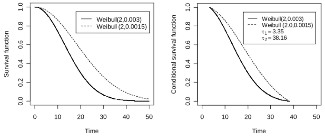
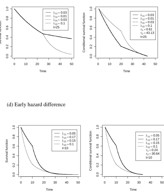
The Weibull distributions with different values of scale parameter and shape parameter are selected for power comparison. Note that the Weibull distribution is a natural model for generating the proportional or nonproportional (crossing) hazards models. In addition, piecewise exponential distributions with different hazards at different time periods corresponding to early or late hazard differences are also selected for power comparison. The survival functions and its conditional survival functions of these alternatives in the same observable range are presented in Figure 3. The conditional survival functions are derived from (1), where u and v are substituted by and1 which are estimated2 from 1,000 simulation runs for each case.
Two types of truncation distributions are considered to examine the effect of truncation patterns on the proposed test statistics. Once the distributions of construction date are determined, the truncation distributions of U and V are obtained. The exponential distributions with scale parameters 0.05 and 0.04 are
used to generate the construction dates for the first and second samples, respectively. In addition, the uniform distribution in the range (0, R), where R=50 and R=30, is employed to generate the construction dates for the first and second samples, respectively. The left and right truncated proportions under the null hypothesis for each configuration are listed in Table 2. The largest and smallest total truncation proportions are around 70% and 40%, respectively.
All comparison results are summarized from 1,000 simulation runs under the significant level = 0.05. Therefore, the standard error for the estimated type I error rate is around 0.0068. To understand the performance of the test statistic without adjusting for the truncation effect, the original logrank test is also investigated in the simulation.
Table 2 lists the type I error rates from the four test statistics; the original logrank test (LR) and logrank test based on estimated number of subjects at risk (LR_E), and the modified weighted logrank test (WLR_M), and the IWD test, under two truncation patterns with 100 observations in each sample. Three weight functions; constant, decreasing and increasing weight functions, are investigated for both proposed tests. Note that the type I error rates from unequal sample size configurations are similar to the results listed in Table 2.
Hence, these results are not shown due to limited space. As expected, the type I error rate of the LR_E test is higher than the nominal level, indicating the importance in deriving the correct variance formula for the LR_E test. When the two groups have different truncation patterns, the original logrank test is a biased test, since its type I error rate becomes very large. The proposed tests WLR_M and IWD have reasonable type I error rates for all the weight functions examined here, except in two cases. However, when the sample size increases to 150 observations in each sample, the type I error rate of the WLR_M test with
constant weight becomes stable.
(Table 2 is about here)
Since the LR and LR_E are biased tests, Table 3 only displays the powers of the two proposed tests under unequal truncation patterns with 100 observations in each sample. As expected, the weighted logrank test with constant weight has better power than the IWD test with constant weight for the alternative demonstrated in Figure 3(a), which is the Weibull proportional hazards model.
On the other hand, the power of the IWD test with constant weight is higher than that of the WLR_M test with constant weight for the Weibull nonproportional alternative plotted in Figure 3(b) under the exponential truncation pattern, whereas the power of the IWD test with constant weight is lower than that of the WLR_M test with constant weight under uniform truncation pattern. It is interesting to note that the WLR_M with conditional survival function estimate Sˆ(t) based on pooled samples as decreasing weight function has higher power than the IWD test with constant weight. This suggests that both tests may gain efficiency with an appropriate or optimal weight function.
In addition, the WLR_M test with constant weight performs better than the IWD test with constant weight for the late hazard difference alternative in Figure 3(c), while the IWD test with constant weight performs better than the WLR_M test with constant weight test under early hazards difference alternative in Figure 3(d) under both exponential and uniform truncation patterns. Although, the plot of survival functions in Figure 3(c) displays a significant late survival difference, two truncated conditional distributions shows large middle survival difference.
Therefore, the increasing weight function 1Sˆ(t) is not able to help detecting such difference, especially, for the WLR_M test.
(Figure 3 and Table 3 are about here)
7.
Concluding RemarksThis paper extends the weighed logrank test and weighted Kaplan-Meier test (or integrated weighted difference test) for doubly truncated data. Note that the former is a rank-based statistics, while the latter is a non-rank based statistic, which can be interpreted as the difference in mean lifetimes. Moreover, the weighted Kaplan-Meier test is more sensitive to the magnitude of the survival difference and to the alternatives with a lag time. To gain efficiency, an appropriate weight function can be chosen for both tests in detecting a particular alternative based on the plot of truncated estimated conditional survival functions. A useful class of weight functions for weighted logrank tests can be found in Fleming and Harrington (1991), whereas the appropriate weight functions for the IWD test can be found in Petroni and Wolfe (1994) and Gu et al.
(1999).
Without incorporating the weight function in both tests, the simulation results indicate that the WLR_M test should be used under the proportional hazards model and late hazard difference alternatives, while the IWD test has more power to detect the early hazards difference alternative. However, for the crossing hazards differences, the IWD test is better than WLR_M test under exponential truncation pattern but the WLR_M test is better than the IWD test under uniform truncation pattern.
R
EFERENCESAlioum, A. and Commenges, D. A. (1996). Proportional hazards model for arbitrarily censored and truncated data. Biometrics 52, 512-524.
Bilker, W. B. and Wang, M. C. (1996). A semiparametric extension of the Mann-Whitney test for randomly truncated data. Biometrics 52, 10-20.
Efron, B. and Petrosian, V. (1999). Nonparametric methods for doubly truncated data. Journal of the American Statistical Association 94, 824-834.
Fleming, T.R. and Harrington, D.P. (1991). Counting processes and survival analysis. New York: Wiley.
Gu M., Follmann D., Geller N. L. (1999). Monitoring a general class of two-sample survival statistics with applications Biometrika 86, 45-57.
Lagakos S.W., Barraj L.M., de Gruttola V. (1988). Nonparametric analysis of truncated survival data, with application to AIDS. Biometrika 75, 515-523.
Lynden-Bell, D. (1971). A method of allowing for known observational selection in small samples applied to 3CR quasars. Monthly Notices of the Royal Astronomical Society 155, 95-81.
Pepe, M. S. and Fleming, T. R. (1989). Weighted Kaplan-Meier Statistic: A Class of. Distance tests for Censored Survival Data. Biometrics 45, 497-507.
Petroni, G. R. and Wolfe, R. A. (1994). A two-sample test for stochastic ordering with interval-censored data. Biometrics 50, 77-87.
Tsai, W. Y. and Zhang, C. H. (1995). Asymptotic properties of nonparametric maximum likelihood estimator for interval truncated data. Scandinavian journal of statistics 22, 361-370.
Turnbull, B. W. (1976). The empirical distribution function with arbitrarily grouped, censored and truncated data. Journal of the Royal Statistical Society, Series B 38, 290-295.
Vardi, Y. (1985). Empirical Distributions in selection bias models. The Annals of Statistics 13, 178-203.
Wang, M. C. (1991). Nonparametric estimation from cross-sectional survival data. Journal of the American Statistical Association 86, 130-143.
APPENDIX A: THE COMPUTATIONAL FORMULA OF THE
COVARIANCE
Coˆv
S~i(y(j)),S~i(y(h))
The covariance between Pˆ andij Pˆ:ih
For the ith sample, the jth row and hth column in the observed Fisher information matrix is
h j F if
Q Q P
y y I
h j F if
Q P
y y I P
y y I
P P
L
i i
i i
i
n
k ik
ihk m ijk
j ij n
k
i ik
n
k ik
m ijk
j ij n
k
i ik
ij n
k
j i ik
ih ij
1
2
2 2 1
) 1 (
1
2
2 2 1
) 1 ( 2
1
) (
2
1 )
1 (
] [
1 )
1 (
] [
] [
ln
where
k i ijk
k i ijk
ijk if J J
J J Q if
1 1
, 0
,
1 , j2, 3, , m。
Thus Coˆv(Pˆij,Pˆih) is the jhth element of the inverse of the observed Fisher information matrix.
For the ith sample, the truncated estimated conditional survival function evaluated at the event time y( j) can be expressed as
) ˆ( ) ˆ(
) ˆ( ) ˆ( )
~ (
2 1
2 )
( )
(
i i
i j i j
i S S
S y y S
S
For notion simplicity, let Hˆ=ij ˆ( ) ˆ( )
2 )
(j i
i y S
S , and Hˆ=i ˆ( ) ˆ( )
2
1
i
i S
S , then
i ij j
i H
y H
S ˆ
ˆ )
~ (
)
(
Thus
~( ),~( )
ˆvS y(j) S y(h) o
C =
i ik i ij
H H H v H o
C ˆ
ˆ ˆ, ˆ ˆ
By the delta method, the above covariance can be expressed as
4 3
3
2 ˆ
ˆ) ˆ( ˆ ˆ ˆ
ˆ) ˆ, ˆ( ˆ ˆ
ˆ) ˆ, ˆ( ˆ ˆ
ˆ) ˆ, ˆ(
i i ih
ij i
i ih ij
i i ij ih
i ih ij
H H r a V H H H
H H v o C H H
H H v o C H H
H H v o
C
where the covariance of Hˆ andij Hˆ can be computed by the formulaih
Hij Hih
v o
Cˆ ˆ, ˆ =Coˆv
Sˆi(y(j))Sˆi(2),Sˆi(y(h))Sˆi(2)
=Coˆv
Sˆi(y(j)),Sˆi(y(h))
Coˆv
Sˆi(2),Sˆi(y(h))
Coˆv