Department of Civil Engineering College of Engineering
National Taiwan University Master Thesis
;
Incorporating the particle memory effect under the impact of turbulence structures into suspended sediment transport analysis:
Toward a novel random walk model
Shih-Hsun Huang
Advisor: Christina W. Tsai, Ph.D.
107 7
July, 2018
、 、
、
: :
。 (the
advection-diffusion equation) 、
—— (the diffusion coefficient)——
/
/ (random walk theory) / ! (the
Stochastic Diffusion Particle Tracking Model)
/
(the jump process) , (the
Weiner process) /
;
: /
/
/ ;
Abstract
In the conventional analysis, suspended sediment transport is regarded as an advection-diffusion process, called turbulent diffusion, which is driven mainly by turbulence. A fairly good estimate of long-term average sediment concentration can be obtained using the advection-diffusion equation. This governing equation is widely applied for the simulation of morphology development, assessment of reservoir lifespan and so on. In hydraulic engineering, the diffusion coefficient is typically calibrated against the data, but the calibration of the diffusion coefficient is not based on the movement of particles, so the estimation of this parameter is a “black box”. Random walk theory provides a way to simulate the probabilistic trajectory of sediment particles in turbulent diffusion; however, the provided sample path may not be consistent with other physical properties of interest, such as velocity fluctuations of the sediment particles because the currently random walk model is based on the advection-diffusion equation:
The second statistical moment of particle displacement is proportional to time and the spreading rate depends on the diffusion coefficient.
To fill the gap between simulated particle velocity and the real flow velocity, and to explain the linkage between single particle movement and evolution of sediment concentration, two random walk-based models are proposed in this study. At first, the jump process is introduced in the stochastic diffusion particle tracking model to delineate the influence of two flow structures, called ejection and sweep events, in the near wall region on suspended sediment transport. The results of simulation demonstrate that the
temporal scale of flow structures plays an important role in carrying sediment particles in suspension. Then, the mathematical impact of including the temporal scale of turbulence coherent structures in the random walk-based model is discussed in terms of memory effect. A novel stochastic process is proposed to analyze the relationship between the probability properties of turbulence velocity and the spreading behavior of the fluid particles. Based on the proposed stochastic process, an improved random walk model of suspended sediment transport is suggested.
Keywords: suspended sediment transport, turbulent diffusion, random walk theory, memory effect, temporal scale of turbulence motion
Contents
... #
... i
... ii
Abstract ... iii
Contents ... v
List of figures ... ix
List of tables... xi
Chapter 1. Introductions ... 1
1.1 Problem statement ... 3
1.2 Research hypotheses ... 5
1.3 Overview of the thesis ... 6
Chapter 2. Literature review ... 8
2.1 Motivation ... 8
2.2 Basic concepts concerning suspended sediment transport ... 8
2.3 Brief introduction to stochastic modeling ... 11
2.3.1 Markov process and the differential Chapman-Kolmogorov equation ... 11
2.3.2 Langevin equation and the Wiener process ... 13
2.3.3 Definition of stochastic integration ... 14
2.3.4 The linkage between Langevin equation and Fokker-Plank equation in
suspended sediment transport ... 16
2.4 Studies of turbulent flow structures ... 19
2.5 Conclusions ... 23
Chapter 3. Modeling suspended sediment transport under the influence of turbulent ejection and sweep events ... 25
3.1 Motivation ... 25
3.2 Methodology ... 26
3.2.1 Construction of flow configuration ... 28
3.2.1.1 Determination of vertical location and duration of event occurrences ... 29
3.2.1.2 Sampling of magnitudes of velocity components for each event ... 33
3.2.1.3 Quantification of diffusion terms after jump terms have been determined ... 34
3.2.2 Simulation of suspended sediment transport ... 36
3.3 Results and discussion ... 38
3.4 Conclusions ... 48
3.5 Recommendation for the next section and future work ... 50
Chapter 4. Incorporating the particle memory effect under the impact of turbulence
structures into suspended sediment transport modeling ... 53
4.1 Motivation ... 53
4.2 Theoretical development ... 58
4.2.1 One-dimensional random walk with controllable persistence on an infinite lattice ... 58
4.2.2 Brownian motion with random time interval ... 65
4.3 Implementation of random time interval Brownian motion: construction of random walk-based model for transport of suspended sediment in open channel flow ... 75
4.3.1 Construction and preliminary implementation of novel random walk-based model ... 76
4.3.1.1 Mean flow velocity ... 76
4.3.1.2 Particle settling velocity ... 77
4.3.1.3 Parameters of Brownian motion with random time interval ... 77
4.3.1.4 Pickup probability ... 81
4.3.2 Results and discussions ... 83
4.4 Conclusions ... 85
4.5 Recommendations for future work ... 89 Chapter 5. Conclusions ... 91 Reference ... 93
List of figures
FIGURE 2.1 Quadrant analysis of velocity fluctuations. ... 20
FIGURE 2.2 Study framework ... 24
FIGURE 3.1 Probability density functions of duration for ejection and sweep events and the maximum height that are reached by the long structures. ... 31
FIGURE 3.2 Conceptual vertical section with an ejection event. ... 32
FIGURE 3.3 Determination of time and space occupied by events in conceptual vertical section. ... 35
FIGURE 3.4 Construction of flow velocity fluctuation time series at one recording point. ... 35
FIGURE 3.5 Fitting results for semi-theoretical curves of turbulence intensities and Reynolds stress. ... 39
FIGURE 3.6 Histograms of stream-wise velocity fluctuation at y = 0.2 δ. ... 41
FIGURE 3.7 Histograms of wall-normal velocity fluctuation at y = 0.2 δ. ... 41
FIGURE 3.8 Histogram of instantaneous Reynolds stress at y = 0.2 δ. ... 42
FIGURE 3.9 Magnitudes of fitted Dv fitted based on various values of dt. ... 44
FIGURE 3.10 One of the sample path in the simulation for particles with ρs = 1.2 and ds = 0.25mm. ... 45
FIGURE 3.11 Results of sediment transport simulations for sediment particles with ρs = 1.2, different diameters ds and settling velocity ws. ... 45 FIGURE 3.12 Result of simulation for particles with ρs = 1.2 and ds = 0.25mm in
which all flow motions are represented by the diffusion terms ... 47
FIGURE 4.1 Sample paths of proposed random walker ... 60
FIGURE 4.2 Development of walker location probability at t = 0,1,4,100. ... 62
FIGURE 4.3 Second moment of walker displacement ... 64
FIGURE 4.4 Schematic diagram of stochastic process ξ(t) in t and τ space ... 67
FIGURE 4.5 Numerical simulations of observed first two moments of ξ(t) time series. ... 69
FIGURE 4.6 Example of determining slope of second moment in numerical simulations. ... 72
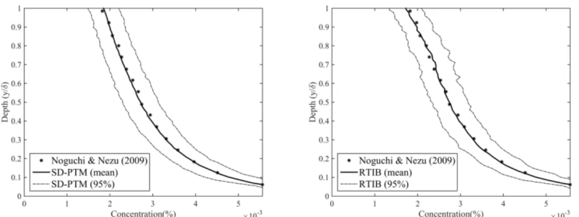
FIGURE 4.7 Turbulence intensity measured in experiment of Noguchi & Nezu (2009). 78 FIGURE 4.8 Fitted mean and standard deviation of qk ... 81
FIGURE 4.9 Simulated and measured sediment concentration profiles in experiment of Noguchi & Nezu (2009). ... 83
FIGURE 4.10 Sample paths of particles with ρs = 1.2 and ds = 0.25mm. ... 83
FIGURE 4.11 The diffusion coefficient calculated using (4.18) and the diffusion coefficient fitted from simulated sediment concentration profile. ... 85
List of tables
TABLE 3.1 Hydraulic conditions in experiment of Noguchi & Nezu (2009) ... 37 TABLE 4.1 Simulation results of integration of ξ(x) with various sets of σ and qk. . 73
Chapter 1. Introductions
Sediment transport in open channel flow has a great impact on siltation of rivers, reservoirs and artificial channels, and it is therefore one of the major topics studied in the hydraulic realm. In spite of the intensive investigation done in the past, the transport mechanism of sediment particles in open channel flow is still not fully understood owing to the chaotic behavior of turbulence, complex interaction between solid and flow phases, effect of sediment grain size distribution and so on. According to the transport mechanism, the processes of sediment transport can be roughly classified into two categories, bed load transport and suspended sediment transport. There are different standards can be used to divide two kinds of transport, in general, bed load transport usually includes unneglectable turbulence modulation (caused by the form drag of sediment particles) and heavily interacts between sediment particles and channel boundary. On the contrary, suspended sediment transport is dominated by the flow properties, i.e. movements of sediment particles follow closely to the flow motion. This study focuses on the suspended sediment transport under dilute situation in open channel flow in which the influence of sediment particles on flow and interaction between particles play minor roles in the overall process.
In the conventional analysis, suspended sediment transport is regarded as an advection-diffusion process, called turbulent diffusion, which is driven mainly by turbulence. In steady state, distribution of sediment particles along with a vertical section can be seen as the result of equilibrium between particle downward intention caused by
gravity and the spread of particles which is disturbed by turbulence. If the location of sediment particles can be described in terms of sediment concentration and present turbulent eddy viscosity as the degree of turbulence disturbance, the celebrated Rouse profile can be derived. As such, a fairly well estimation of long term average sediment concentration can be obtained. On the other hand, as the governing equation of suspended sediment transport in unsteady flow, the advection-diffusion equation is widely applied for the simulation of morphology development, assessment of reservoir lifespan and so on.
Nevertheless, when it comes to conducting a more delicate analysis of suspended sediment transport, a deterministic estimation is no longer satisfactory. To get advanced information, researchers introduce the probabilistic concept to the analysis of suspended sediment transport. One of them linked the Langevin equation with the advection- diffusion equation through Fokker-Plank equation and developed the stochastic particle tracking model (a detailed derivation will be provided in §2.). The model illustrates the probabilistic trajectory of sediment particles in each realization and provides a bridge from the behavior of individual sediment particles to diffusion phenomena of sediment concentration. It shows the assumptions implied in the advection-diffusion equation, a so-called Fickian assumption and memoryless property. Apart from the Fickian assumption that describes the behavior of particle spreading, memorylessness is another important assumption about the transition of system between different states. In short, it
is referred to as the statement that future status of system is only dependent on its current status.
However, studies of wall-bounded turbulence, the turbulence in boundary layer, pipe, and open channel flow, indicate the existence of coherent structures which have their own
“order” to form, develop, and dissipate. This “order” implies the appearance of temporal and spatial correlations among flow properties (Nezu & Nakagawa 1993). The anisotropy and inhomogeneity of turbulence coherent structures make the traditional Gaussian random walk incompatible with the path that sediment particles actually take (Adrian &
Marusic 2012). Thus, it is desirable to refine the model based on the random walk theory to provide more realistic simulation of suspended sediment transport and meanwhile to keep its conciseness without involving moment or force balance equations.
1.1 Problem statement
As mentioned previously, the Rouse profile yields results that are consistent with experimental and field data in long term average and the advection-diffusion equation is applied to various engineering implementations. However, even in the steady state, sediment concentrations will fluctuate because large turbulence eddies, or the so-called turbulence coherent structures disturb sediment particles (Cellino & Lemmin 2004).
It shows that the diffusion based models only fit the bulk/long-term-average phenomena of the turbulent diffusion, and some behaviors of suspended sediment
transport are missing. All the factors that influence the spreading of the sediment particles are lumped in one important parameter, i.e., the sediment diffusion coefficient. The non- clearance of the mechanism works behind the coefficient makes it hard to be determined without the aid of fitting or regressing with the data when the predicted sediment concentration of the diffusion based model deviates from the reality.
Despite turbulence motions are chaotic, the motions have a local trend and correlation in time and space owing to the existence of large eddies. Statistical properties of the turbulence structures may give information of suspended sediment particle movement in the flow field. Once the movement of suspended sediment particles can be illustrated, the physical meaning of the sediment diffusion coefficient can be revealed. In addition, the correlations between sediment flux and the turbulence coherent structure have been reported in experiments (Noguchi & Nezu 2009; Salim et al. 2017). Turbulence coherent structures should be more comprehensively considered in the sediment transport model if at all available.
The aim of this study is to better investigate the role of the sediment diffusion coefficient on suspended sediment particle movement in open channel flow. Meanwhile, a novel stochastic process that incorporates the memory effect to represent the turbulence flow structure will be introduced. An improved random walk model based on this process is suggested.
1.2 Research hypotheses
The turbulence structures contribute to the local trend of the flow and sediment particle movements. Whether the effect of the local trend will remain in the long term phenomena is another story. For example, in the near wall region of wall bounded turbulence, the turbulence coherent structures of the ejection and sweep events are associated with sediment entrainments and affect the instantaneous local sediment concentration (Dwivedi et al. 2011; Rashidi et al. 1990;); notwithstanding, such events are highly intermittent and sporadic. The conventional analysis based on the advection- diffusion process can give a fairly well estimation of long term average concentrations.
The importance of these events in the explanation of the relationship between the bulk diffusion phenomena and single sediment particle movements in sediment transport is questioned.
Moreover, when the turbulence coherent structure disturbs the sediment particles, particles seem to be carried by the flow at longer time scales, which differ from the Kolmogorov time scale that is used in the simulation of the particle tracking model. Is it merely the property of coherent structure that is not worth mentioning in the overall transport mechanism? Or it has a profound physical meaning for flow to carry particles in suspension? With respect to the entrainment of particles from the river bed, the intensity of flow events is not the only factor that determines whether a particle is picked up. The temporal scale of the flow events is also important (Dwivedi et al. 2011). The situation may be similar for particle moving in flow fields.
Thus, the two hypotheses that are considered in this study are as follows.
1. The ejection and sweep events in the near wall region affect long-term average sediment concentrations.
2. The temporal scale of the flow events is essential to understanding the relationship between the turbulent diffusion and turbulence intensity.
Both of the hypotheses are related to the descriptions of sediment particle movement in the turbulence diffusion. After verifying the two hypotheses, the necessity of introducing a novel framework of the stochastic particle tracking model for suspended sediment transport that can represent the existence of the flow structures in open channel flow will been shown.
1.3 Overview of the thesis
The background knowledge and the connections of this study with existing work will be mentioned in §2. After that, two sections follow, modeling suspended sediment transport under the influence of turbulent ejection and sweep events and incorporating the particle memory effect under the impact of turbulence structures into suspended sediment transport modeling. Two sections are contained in §3 and 4 respectively. At the end, the overall conclusions will be provided in §5.
At the first section of the thesis, the temporal scale of large flow events is incorporated into the stochastic particle tracking model. As the first attempt to consider
the random walk based model of sediment transport with turbulence coherent structures, this study focuses on the ejection and sweep events which are related to the hairpin vortex in the near wall region. The results of simulation demonstrate that the temporal scale of flow structures plays an important role in carrying sediment particles in suspension.
In the second section, the mathematical impact of including temporal scale of turbulence coherent structures in the random walk based model is discussed in terms of memory effect. A novel stochastic process is proposed to analyze the relationship between the statistical properties of turbulence velocity and the spreading behavior of the fluid particles. Based on the process, the framework of a new random walk model for suspended sediment transport is suggested.
Chapter 2. Literature review
2.1 Motivation
The basic concepts of conventional analysis of suspended sediment transport, relative stochastic modeling, and the study of turbulence coherent structures are mentioned in this chapter. The aim of these descriptions is to illustrate an overall picture about how this study approaches its final goal: Discuss the in-depth physical interpretation of sediment diffusion coefficient for suspended sediment movement in open channel flow. Based on the interpretation, a novel random walk model can be proposed.
The previous studies using the mathematical equivalent between the advection- diffusion equation and stochastic modeling to abstract the information of the sediment particle trajectory in turbulence. Let the statistical properties of particle movements in stochastic modeling be consistent with the statistical properties of flow motion, the simulated sediment concentration profiles will depict the relationship between a single sediment particle movement and the bulk diffusion phenomenon.
2.2 Basic concepts concerning suspended sediment transport
Suspended sediment transport is regarded as an advection-diffusion process in conventional analysis. Assuming that particle movement driven by the concentration
gradient against the particle settling velocity in equilibrium yields the following governing equation for the vertical direction.
<=> ? = @=ABC(A)
BA , (2.1)
where <= denotes the particle settling velocity; > is the sediment concentration, and
@DE is the particle diffusion coefficient in the vertical direction. Rouse (1937) assumed that particle diffusivity is equivalent to turbulent eddy viscosity FG,
@=A ≈ FG = IJ∗? 1 −MA . (2.2)
Then the classical Rouse vertical concentration profile can be derived as
C(A)
CNO = MPAMPA
O AO
A QR
ST∗, (2.3)
for ? > ?V, where I is von Karman constant; J∗ is friction velocity of open channel flow; W is water depth; ?V is the reference height, and >AO is sediment concentration at reference height. The exponent of the right-hand side of (2.3) is known as Rouse number which is one of the indicators for the discrimination of bed load particles and suspended load particles. As long as fine and light particles are considered, the Rouse profile yields results that are consistent with experimental and field data. When a small deviation from the Rouse profile occurs, data can be refitted by adding a universal ratio X or the reciprocal of the Schmidt Number YZG, of the fluid eddy viscosity to the particle diffusivity
X =\][
^= _`RN
^. (2.4)
Therefore, the Rouse profile can also be used as a tool to verify against relevant experimental results in various studies.
In fact, the above governing equation (2.1) is the one-dimensional advection- diffusion equation in steady state. The general from of the advection-diffusion equation for suspended sediment transport is
aC
aG = ∇ c=⋅ ∇> − (e + gD)∇> + Y h, i , (2.5) where ∇ is divergence operator; c= is sediment particle diffusivity in vector form; e is mean flow velocity; gD is sediment particle settling velocity which has value only in the vertical direction; Y is the source of sediment particles that means the particles are released at h when time i. The advection-diffusion equation has been wildly applied in the simulations of suspended sediment transport for assessment of water quality, simulation of morphology development, estimation of reservoirs and so on.
To improve the accuracy of simulation, many investigations have focused on refining estimates of the eddy viscosity and the Schmidt Number. For example, Toorman (2008) solved mass and momentum conservation equations for two-phase flow, and proposed an analytical formulation of the Schmidt number. Absi, Marchandon & Lavarde (2011) calibrated the formula of eddy viscosity using the direct numerical simulation data.
Numerous studies have also considered the turbulence modulation.
However, little has been done to discuss the relationship between the turbulent eddy viscosity and sediment particle diffusivity. The question about how fluid momentum transfer drives sediment particle mass transfer is unanswered. Fortunately, the random walk theory provides a mathematical way to assess particle movements. Movements that follow Brownian motion can lead to a diffusion process. A brief introduction of stochastic modeling and its linkage with the advection-diffusion equation are mentioned below.
2.3 Brief introduction to stochastic modeling
2.3.1 Markov process and the differential Chapman-Kolmogorov equation
Generally, the purpose of stochastic modeling is to describe a system transits between different states with probabilities, and stochastic process is a system that evolves probabilistically in time. Markov process is a kind of stochastic process with broader implements. The formulation of transition probability for Markov process relies on the memoryless assumption which refers to the fact that the future state of the system depends only on its most recent state, i.e.,
j k[, i[; km, im; … ?[, o[; ?m, om; … = j k[, i[; km, im; … ?[, o[ , (2.6) for i[ ≥ im ≥ ⋯ ≥ o[ ≥ om…, where j is the conditional probability of system state;
k[, km, … is the predicted values of the system state which is a time dependent random variable r(i) at time i[, im, … , and ?[, ?m, … is the known values of r(i) at time
o[, om, … .
The relation can lead to Chapman-Kolmogorov equation
j k[, i[ ks, is = j k[, i[; km, im ks, is tkm
P
= j k[, i[ km, im; ks, is j km, im ks, is tkm
P
= P j k[, i[ km, im j km, im ks, is tkm. (2.7)
Consider the time evolution of Chapman-Kolmogorov equation then the differential Chapman-Kolmogorov equation arises (Gardiner 1997),
u
uij v, i w, ix = − u
uyz {z v, i j v, i w, ix
z
+ um
uyzuy| }z| v, i j v, i w, ix
z,|
+ ~ v , i j , i w, ix − ~ v, i j v, i w, ix t, (2.8)
for i > ix, where j v, i w, ix is the conditional probability that state of system is v at time i if the state of system is w at ix; the first two terms of the right hand side simulate the continuous transition of the state and { v, i and } v, i are the coefficient of the drift term and coefficient of the diffusion term respectively, and the third term of (2.8) simulate the discontinuous transition of the system state. It means the probability that the state transits from to v minus the probability that state transits from v to . The
~ v , i define as
~ v , i ≡ lim
ÉG→Ö
Ü v,GáÉG ,G
ÉG . (2.9)
If the time evolution of the probability can be described using only first two terms on the right hand side of (2.8), the equation is a so-called Fokker-Plank equation,
BGB j v, i w, ix = − BàB
â {z v, i j v, i w, ix
z + BàBä
âBàã }z| v, i j v, i w, ix
z,| . (2.10)
On the other hand, if the time evolution can be described using only the last term on the right hand side of (2.8), the equation is called the Master equation. The above equations are known as the forward Kolmogorov equations.
Note that the Fokker-Plank equation has the similar form with the advection- diffusion equation if the probability j is considered as concentration >. In addition, the Fokker-Plank equation is mathematically equivalent to the Langevin equation, which is a family of stochastic differential equations.
2.3.2 Langevin equation and the Wiener process
The stochastic differential equation with a noise term is known as Langevin equation.
Its general form can be written as
åç
åG = é i, r(i) + è i, r(i) ⋅ ê(i), (2.11) where r is a stochastic process; é, è are given functions, and êG is an ideal noise term.
If it is used to simulate the stochastic process such as Brownian motion, êG has following properties (Øksendal 1998),
1. ê(i) = 0 for all i.
2. ê(i)ê(ix) = ë(i − ix).
3. ê(i) is stationary.
where ë is the Dirac delta function. However, the integration of êG in time leads to a contradictory consequence that
ê(í)tí
G (2.12)
is a Wiener process ì(i) and it is nowhere differentiable.
The Wiener process mentioned here has a few properties as follows.
1. ì(0) = 0 with probability 1.
2. It has stationary independent increment. îì îi = ì i + îi − ì i is independent of i.
3. îì îi ~ê(0, îi). The increment follows normal distribution with mean zero and standard deviation îi.
To interpret the integral consistently, rewrite (2.12) in discrete version and replace ê i îi with îì i ,
r iñ = rÖ+ ñP[|óÖé i|, r i| îi| + ñP[|óÖè i|, r i| Δì(i|). (2.13)
that îì i| is defined as îì i| = ì i|á[ − ì i| . If îi| → 0 , the usual integration notation can be used
r i = rÖ+ ÖGé í, r í tí+ ÖGè(í, r(í))tì(í). (2.14) Before further analysis, the above integral needs to be defined. It has to be known that the value of ÖGè(í, r(í))tì(í) will depend on the selected integral scheme. The most two well accepted schemes are Ito calculus and Stratonovich calculus.
2.3.3 Definition of stochastic integration
Define the stochastic integral GG è(í)tì(í)
ô as
öñ = ñ|ó[è o| ì i| − ì(i|P[) , (2.15)
where iÖ ≤ i|P[ ≤ o| ≤ i| ≤ i. The chosen of o| will decided the result of integration.
For example, for Stratonovich calculus o| =GãáGmãúù is specified and thus,
ö = Gì í ∘ tì í
Gô
= üí−lim
ñ→
ì i| + ì i|P[
2 ì i| − ì i|P[
ñ
|ó[
=[m ì iÖ m− ì i m , (2.16)
where the symbol ‘∘’ is used to indicate that the integral is defined based on the Stratonovich integral scheme, and üí−†°ü is referred to as the mean square limit that üí−lim
ñ→ rñ = r if
ñ→lim j ¢ rñ ¢ − r ¢ mt¢ = 0. (2.17)
¢ is the event in a probability space £, and j(¢) is the probability that ¢ happens.
On the other hand, for Ito calculus o| = i|P[ is specified,
öñ = ì i|P[ ì i| − ì i|P[
ñ
|ó[
≡ ì i|P[ îì i|
ñ
|ó[
= 1
2 ì i|P[ + îì i| m− ì i|P[ m− îì i| m
ñ
|ó[
= 1
2 ì i| m− ì i|P[ m− îì i| m
ñ
|ó[
=[
m ì i| m− ì i|P[ m −[
m ñ|ó[îì i| m, (2.18)
where ñ|ó[îì i| m = ñ|ó[ ì i| − ì i|P[ m = ñ|ó[(i|− i|P[) = i − iÖ. Thus,
ö = GGì(í)tì(í)
ô =[m ì iÖ m − ì i m− (i − iÖ) . (2.19) It is different from the result which is calculated based on the Stratonovich integral scheme. The Ito scheme is chosen here to show the linkage between the Langevin equation and Fokker-Plank equation for convenience.
2.3.4 The linkage between Langevin equation and Fokker-Plank equation in suspended
sediment transport
Consider a Langevin equation in Ito scheme,
tk i = § k, i ti + • k, i tì i , (2.20) where k(i) which is a function of time i; § k, i and • k, i are given functions, and ì i is Wiener process. To find a differential of a time-dependent function that involves a stochastic process, introduce Ito formula. Let é(k) be a function of k, expand té(k) by Taylor’s series to the second order and substitute the Langevin equation to tk.
té k = é k + tk − é k = éx k tk +1
2éxx k tkm+ ⋯
= éx k § k, i ti + • k, i tì i +[méxx k • k, i mti + ⋯, (2.21) thus,
té k = § k, i é′(k) +[m• k, i mé′′(k) ti + • k, i éx k tì i , (2.22)
which is Ito formula. Note that tim → 0, titì i → 0, and tì i m → ti. Using Ito formula to consider the time development of an arbitrary function é k , i.e. the time variation of é k , one can obtain
åß ®
åG = åß ®åG = åGå é k . (2.23)
On the other hand,
åß ®
åG = § k, i é′(k) +[m• k, i mé′′(k) . (2.24) According to the above equations, use the definition of expected value and denote j k, i kÖ, iÖ = j,
t
ti é k = é k uj
uitk
P
= § k, i éx k +1
2• k, i méxx k uj uitk
P
= § k, i é k j +1
2• k, i méx k j − é k u uk
• k, i m
2 j
=©™ß´]¨
+ é k
P
− u
uk§ k, i j + um ukm
1
2• k, i mj tk
= P é k −B®B § k, i j +B®Bää[m• k, i mj tk. (2.25)
Note that j vanishes in surface terms ( k → ± ⟹ j → 0 ). The equivalence between line 1 and line 4 of (2.25) holds for arbitrary function é k . It implies that
BÜ ®,G ®ô,Gô
BG = −B®B § k, i j k, i kÖ, iÖ +B®Bää [m• k, i mj k, i kÖ, iÖ . (2.26) Comparing to the Fokker-Plank equation (2.10) in a univariable problem, one obtain
−§ k, i = { k, i ,
[
m• k, i m = } k, i , (2.27 a,b)
respectively.
For a multivariable Langevin equation
t = Ø , i ti + ∞ , i t± i , (2.28)
where Ø , i and ∞(, i) is a given vector and matrix functions respectively, and t± i is a multivariable Wiener process, the corresponding Fokker-Plank equation is
BÜ
BG = − B®B
â §z , i j
z +[m B®Bä
âB®ã • , i • , i ≤ z|j
z,| , (2.29)
where j = j , i Ö, iÖ).
Contrary to the Fokker-Plank equation, Langevin equation is a Lagrangian equation that follows particle movement. The number of simulated particles represents the probability that particles exist in a particular location. The ensemble of thousands of simulation results yield the probability distribution of particles located in the simulation field. Owing to the enormous number of suspended sediment particles in a real channel, this probability can be treated as the normalized sediment concentration, i.e.
j , i ∝ > , i . (2.30)
The corresponding Langevin equation of the advection-diffusion equation is, t = e + g=+ ∇c= ti + 2c=t± i , (2.31) where e is the average flow velocity; g= is a three-dimensional vector with a non-zero value in the vertical direction, which represents the settling velocity of particles; c= is
the sediment diffusion coefficient in three dimension. The above equation is the governing equation of the stochastic diffusion particle tracking model (SD-PTM) developed by Man & Tsai (2007).
The stochastic diffusion particle tracking model delineate sediment particle trajectory that can lead to turbulent diffusion. The assumptions of the random walk theory are also consistent with Kolmogorov’s turbulence theory; however, wall-bounded turbulence in open channel flow is neither isotropic nor homogeneous. Using the random walk theory to explain the path of a particle may fail to consider all relevant information (Adrian & Marusic 2012). As such, an explanation based on physical concepts may be more useful. Since turbulence is the major driving force of suspended particle movement, a better physical insight into turbulence coherent structure should be desirable.
2.4 Studies of turbulent flow structures
Turbulent coherent structures are generally referred to as parcels of fluid that move and develop with a certain “order”, which implies the existence of temporal and spatial correlations among flow properties (Nezu & Nakagawa 1993). After Kline et al. (1967) described the bursting behaviors in boundary layer flow, studies of the coherent structures in the near-wall region began to be performed. Grass (1971) showed that similar flow features, called ejection and sweep events, are present in wall-bounded turbulence.
Ejection and sweep events occur in the streaks with low and high stream-wise velocities respectively (Rashidi, Hetsroni & Banerjee 1990). In addition to the directions of relative
motions, these events are also associated with a high local instantaneous Reynolds stress
−J′¥′ (Noguchi & Nezu 2009). Most of the techniques that are used in experiments to distinguish ejection and sweep events from velocity fields are based on the aforementioned characteristics. Consider quadrant analysis as an example. If the velocity fluctuations of those events are plotted on a J′¥′ plan, as shown in figure 2.1, then the ejection and sweep events can be seen to be Q2 and Q4 motions, respectively (Nezu &
Nakagawa 1993). Other than quadrant analysis, the correlation in flow velocity/pressure time series, the swirling of the flow, are used to indicate the existence of the coherent structures in the boundary layer flow and wall-bounded turbulence (Sillero, Jimenez &
Moser 2014; Chong et al. 1998; Lehew, Guala & McKeon 2013).
FIGURE 2.1 Quadrant analysis of velocity fluctuations;
weaker signals that fall in the ‘hole’ will be filtered out.
This figure is modified from Nezu & Nakagawa (1993).
When the emphasis is placed on the motion of eddies, another remarkable structure can be found in the near-wall region. First identified by Theodorsen (1952), it has been called the horseshoe, π, Λ, or hairpin vortex, based on its observed shapes. Various explanations of the relationship between ejection/sweep events and the hairpin vortices have been offered. One of them is that ejection and sweep events are in different stages
of vortex development, implying that ejection and sweep events happen consecutively (Kaftori, Hetsroni & Banerjee 1995; Salim et al. 2017). Another involves the attached eddy hypothesis that was originally proposed by Townsend (1976), according to which, vortices that are rooted in the near-wall region are particularly important. In a figure that was drawn by Marusic & Woodcock (2016), the flow regions with low/high stream-wise velocity compare to the mean flow velocity profile are inside and outside of the flow field, which is generated by a representative eddy. Furthermore, hairpin vortices normally are grouped together and form large flow structures, called hairpin vortex picket. Multiple packets will further align to form very large scale motions in the logarithmic region (Dennis 2015).
In the work of Dennis & Nickels (2011a, b), the spatial relationships between the hairpin vortices and very large scale motions, and between very large scale motions and ejection/sweep events are shown. Their results revealed that very large scale motions with low stream-wise velocities tended to couple with very large scale motions with high stream-wise velocities, but two adjacent structures usually have different properties such as length in stream-wise direction. There is a preferential formation of very large scale motions with low stream-wise velocity in turbulence that the low-speed structure has
“stronger characteristics”.
Most of the discussions about turbulence coherent structures focus on the eddies in the near wall region. Very large scale motions in the other region have been reported in
the boundary layer flow and open channel flow (Adrian, Meinhart & Tomkins 2000;
Hurther, Lemmin & Terray 2007). The motions can also be explained by the hairpin vortex packets as mentioned above; however, Perry & Marusic (1995) extended the attached eddy hypothesis to derive theoretical equations for turbulence intensities and Reynolds stress. They found that the existence of the hairpin vortices alone does not suffice to determine the Reynolds stress. To complete their analysis, the existence of another kind of vortex that is not rooted in the near-wall region is speculated. They called such vortex as ‘detached eddies’ and the hairpin vortex is known as ‘attached eddies’.
Using velocity tenser to identify turbulent structures in the boundary layer, Lehew, Guala & McKeon (2013) defined so-called swirling coherent structures and classified those structures as attached and detached one. The average number of swirling coherent structures decays significantly beyond the logarithmic layer, and the fraction of attached structures also decays with an increasing distance from the wall. Different flow structures dominate in its own specific region, and the statistical properties of flow velocities will change respectively. On the other hand, del Alamo et al. (2006) analyzed the direct numerical simulation data and reported ‘wall-detached/attached vortex clusters’, which have different properties as opposed to those with hairpin vortex.
The existence of other kinds of coherent structure and the impact of external flow in the wake region are unclear. Given the insufficient information about turbulent structures in the outer region, the first section of the study focuses primarily on the influence of
ejection and sweep events, which are associated with very large scale motions with low/high stream-wise velocities and hairpin vortices and its influence on suspended sediment transport have been confirmed (Dwivedi et al. 2011; Rashidi et al. 1990;
Noguchi & Nezu 2009; Slim et al. 2017).
2.5 Conclusions
The study background is briefly introduced in this chapter. It is worth noting that most of the aforementioned analyses are based on Reynolds decomposition that
e = e + ex, (2.32)
where e is total flow velocity; e is mean flow velocity, and e′ is velocity fluctuations.
The advection-diffusion equation uses the diffusion coefficient to present the consequence of sediment particles moved by e′. In the stochastic diffusion particle tracking model, the Wiener process is used to represent e′. e′ has its own distribution;
however, it is not necessarily Gaussian. The distribution of e′ is dependent on the properties of flow structures in the flow field. The statistical properties of flow velocities contain the information of flow particle movement. In this study, such information will be used to represent the flow structures in open channel flow.
The framework of this study is depicted in figure 2.2. Express flow velocity with the aid of Reynolds decomposition and apply two different stochastic processes describe the randomness of the turbulence velocity fluctuations. Assume that the suspended sediment particles exhibit motion very close to turbulence flow, the velocity of the suspended
sediment particles can be obtained as the superposition of flow velocity and sediment particle settling velocity. Then, the simulation of suspended sediment transport in open channel flow than can be conducted. The analysis will be done based on the simulated sediment concentration profile.
FIGURE 2.2 Study framework.
Chapter 3. Modeling suspended sediment transport under the influence of turbulent ejection and sweep events
3.1 Motivation
Suspended sediment transport in open channel flow importantly affects water quality as well as reservoir and river siltation; it has therefore been a subject of intense investigation. In estimating the sediment concentration, suspended sediment transport is regarded as an advection-diffusion process called turbulent diffusion. To elucidate its mechanism, particle behavior is examined. The relationships between movement of a single particle and overall transport phenomena are also of interest. Ancey, Bohorquez &
Heyman (2015) derived the advection-diffusion equation from the forward Kolmogorov equation to determine how parameters of transport processes, such as deposit/entrainment rates and particle velocity fluctuations, contribute to diffusion coefficients. Despite the great effort put into the study of transport mechanism, a full explanation of the linkage between single particle movement and evolution of sediment concentration has not yet been achieved owing to its complicated nature.
This section discusses physical interpretations of turbulent diffusion using the stochastic particle tracking model, which defines diffusion coefficients in terms of particle velocities. The diffusion coefficient of the model is adjusted to fit the turbulence intensity which is the standard deviation of turbulence velocity fluctuations. Two flow
structures, called ejection and sweep events, in the near wall region have been especially focused to delineate the influence of the flow structures on suspended sediment transport.
Ejection events are positive vertical flow motions with a stream-wise velocity that is less than the mean flow velocity; the sweep events are negative vertical flow motions with a stream-wise velocity that exceeds the mean flow velocity. Although ejection and sweep events are thought to be confined to the buffer layer where yá ≤ 30 (Nezu &
Nakagawa 1993, yá = ?/(F J∗)), the occasional occurrence of large ejection events in the outer region has been identified in both experiments and direct numerical simulations (Cellino & Lemmin 2004; del Alamo et al. 2006). These events are associated with sediment entrainments and affect the instantaneous local sediment concentration in the near-wall region (Dwivedi et al. 2011; Rashidi et al. 1990; Noguchi & Nezu 2009; Slim et al. 2017).
3.2 Methodology
Following Reynolds decomposition, flow velocities can be separated into mean velocities and velocity fluctuations. Similarly, the stochastic particle tracking model simulates particle movement as a superposition of drift terms and diffusion terms. It means the movement of sediment particles is modeled via the diffusion process. This study is interested in how the specific flow motions contribute to the transport phenomena on the average. This study also attempts to distinguish the ejection and sweep events from
other types of fluid motions. The diffusion process and the jump process are combined to represent sediment movement influenced by different flow motions.
The flow motions that are directly associated with ejection and sweep events are treated as the jump process and others are treated as diffusion process. A jump process is referred to as a random sequence of sufficiently large, discrete and discontinuous displacements such as a sequence of large random particle displacements, instantaneously taking place within a short period of time, or continuously lasting for a period of time.
The procedure based on the properties of coherent motions of ejection and sweep events and followed by the jump process is listed below.
1. Ejection and sweep events occur randomly. Without the occurrence of these events, there is no velocity and displacement in the jump process.
2. Once these events occur, they last for a period of time; and the duration of each event is considered to be a random variable.
3. In this study, the magnitude is kept constant in an event for the entire event duration for simplicity. Magnitude of different events; however, is a random variable.
4. When integrating the particle velocity over the event duration, particle displacement as depicted earlier in a jump process can be quantified.
The analysis will be performed in two stages, which are construction of the flow configuration and simulation of suspended sediment transport.
3.2.1 Construction of flow configuration
To identify the contribution of ejection and sweep events to suspended sediment transport, the portions of flow particle velocities that are directly related to those events must be separated from those of other velocity component. According to Nezu &
Nakagawa (1993), ejection and sweep events involves the moving together of parcels of fluid for a particular period. If this motion is treated as the jump process, the formula for fluid velocity decomposition can be written as
e = e + ex = e + 2cɱÉG = e + 2πɱÉG + ∫ª(º, ~) (3.1)
where ɱ
ÉG are Gaussian White noise and c are the eddy viscosities. 2πɱ
ÉG are the velocity components that are related to the flow structures other than ejection and sweep events, and they will be called diffusion terms. The magnitudes of π are parameters and will be determined based on velocity fluctuations of turbulence. ∫ are the magnitudes of the events’ velocities and are random variables, called the jump terms; ª(º, ~) is a discriminating function that indicates the existence of ejection and sweep events in a particular location, and the function will depend on º and ~. º follows a Poisson process that º = ºΩ°ííΩæ(ti ~), and it determines whether an event will occur. ti is the time step for simulation, and ~ is the mean period of the ejection and sweep events.
~ is the duration of events which is a random variable. An event may last for longer than a single time step. After the formula for flow velocity has been specified, the following procedure, which has three steps, is implemented. They are (i) to determine the vertical location and duration of each event; (ii) to sample the magnitudes of the velocity
components for each event, and (iii) to quantify the diffusion terms once the jump terms have been determined. At the end of this process, the time series of velocity fluctuations at various flow elevations can be obtained.
For the sake of simplification, ejection and sweep events are assumed to share the same strength/duration distributions. Furthermore, the likelihoods of the occurrences of ejection and sweep events are also assumed to be equal (50%, 50%) for simplicity. The primary difference between ejection and sweep events in this study is in the sign of the velocity fluctuations. The applicability and impact of the above assumptions will be discussed in §3.3.
3.2.1.1 Determination of vertical location and duration of event occurrences
Before the time and space of the flow field occupied by events can be determined, the duration distribution and the spatial distribution of the events should be known.
Though the time-durations of ejection and sweep events pass through a measured point can be detected using quadrant analysis (Katul et al. 1994; Day et al. 2018), the durations that events persist are hard to be decided from a point-wise measurement, as an event may last for a period after passing the measured point. Laskari et al. (2018) studied time evolution of uniform momentum zones in a turbulent boundary layer and provided the residence time of large-scale Q2 and Q4 events which are associated with low-/high- speed structures in their field of view. Despite the residence time of large-scale Q2 and
Q4 events cannot be exactly considered to be the durations of these events, it depicts the property of the persistence of these events. Thus, the residence time is treated as the event duration in this work to illustrate the temporal influence of flow events on sediment particle movement.
In Figure 13 of Laskari et al. (2018), it can be seen that two kinds of events have similar residence time distributions. As the first attempt to consider turbulence coherent structure in the illustration of particle trajectory in suspended sediment transport, this study assumes that the duration distribution of ejection and sweep events to be the same for simplicity. And duration distribution of ejection events as shown in Figure 3.1 is used as the main focus on the upward movement of particles.
With respect to the spatial distribution of ejection and sweep events, Dennis &
Nickels (2011b) analyzed the quasi-instantaneous three-dimensional velocity fields of a turbulent boundary layer, and found that strong vertical velocity fluctuations are adjacent to the large flow structures. Intense upward flow movements are associated with structures with low stream-wise velocity; intense downward flow movements are associated with structures with high stream-wise velocity. It implies that ejection and sweep events occur around structures with low and high stream-wise velocities, respectively. Therefore, the histogram of the maximum height that is reached by the structures with low and high stream-wise velocities is used to represent the probabilities of ejection and sweep events in different flow elevations. The Gamma distribution was
ultimately chosen for representing the histogram provided in Dennis & Nickels (2011b) because of its best fitting. Figure 3.1 displays the probability density functions that are used in this study.
FIGURE 3.1 Probability density functions of duration for ejection and sweep events and the maximum height that are reached by the long structures. Mean duration is 98 iá(iá = i J∗m F).
For steady, uniform, open-channel flow, a conceptual vertical section, as depicted in figure 3.2, is considered. The passing of 1,000 events of each kind through the section is simulated. The Poisson process (Poisson(ti ~)) is used to determine whether an event occurs in each time step. If an event occurs, then its duration must be sampled. The flow region that is lower than the sampled maximum height is affected by the event. A time series of an event’s passing or not for each recording point in the conceptual vertical section is generated. Accordingly, the vertical location and duration of the event occurrences are determined. The purpose of considering the conceptual vertical section is to reduce the effort of sampling random variable. The result will be the same if the process is conducted point by point at each elevation. The space correlation is not included in the following modeling.
FIGURE 3.2 Conceptual vertical section with an ejection event.
3.2.1.2 Sampling of magnitudes of velocity components for each event
Assume that the vertical and stream-wise velocity components that are associated with ejection and sweep events follow normal distributions. Also assume that they are correlated with each other because the events contribute to long-term Reynolds stress.
After the magnitudes of the jump terms for each event are sampled, a time series of the jump terms at each recording point in the conceptual vertical section can be obtained.
The means of the jump terms are zero. However, the standard deviations of the jump terms for each event and their covariance must be determined. Owing to the difficulty of distinguishing the velocities that are associated with ejection and sweep events from those associated with other Q2/Q4 events in the experiments, no direct evidence of the magnitude of the standard deviations of the jump terms can be provided. The reasonableness of these values has to be judged by whether the flow properties in this stage are reasonable and even by whether the sediment concentrations that are provided by the following stage are consistent with experimental data. At this point, the Reynolds stress and the turbulence intensities that are calculated from the jump term time series should not exceed the overall Reynolds stress – J′¥′ and the turbulence intensities in the experiments.
The turbulence intensities are defined as ≈© = Jxm, and ≈∆ = ¥xm. The semi- theoretical curves for turbulence intensities, verified by Noguchi & Nezu (2009) written
below, and the Reynolds stress are used as standards for verifying the standard deviations of the jump terms.
≈© = 2.3J∗«PA », ≈∆ = 1.27J∗«PA », (3.2a,b)
where J∗ is the friction velocity, and ë is the thickness of the boundary layer, which is defined as the region from the channel bottom to the flow elevations where the Reynolds stress equals zero. The theoretical curve for the Reynolds stress is,
−©x∆x©
∗ä = 1 −A» −B©BA , (3.3)
where Já = J J∗ and uJá u?á can be estimated from the log mean velocity profile (3.8).
3.2.1.3 Quantification of diffusion terms after jump terms have been determined
The definition of diffusion terms in the stochastic particle tracking model is utilized to specify fluid particle movements other than those directly related to the ejection and sweep events. The superposition of the diffusion terms and the jump terms yields a time series of velocity fluctuations at each recording point in the conceptual vertical section.
The standard deviation of velocity fluctuations at each recording point is used to fit the semi-theoretical curves of turbulence intensities. An adjustment yields the values of π.
The correlations between diffusion terms are also considered to fit the theoretical Reynolds stress in different flow elevations. Figure 3.3 and 3.4 present the procedure that is carried out in the current stage. The standard deviations of the jump terms and the values of π are used in the following stage.
FIGURE 3.3 Determination of time and space occupied by events in conceptual vertical section.
FIGURE 3.4 Construction of flow velocity fluctuation time series at one recording point.
3.2.2 Simulation of suspended sediment transport
The governing equation for the stochastic diffusion jump particle tracking model is t = (e + g=)ti + 2πt± + ∫ª º, ~ ti, (3.4) where is particle position; t± are the Wiener process; g= is a three-dimensional vector with a non-zero value in the vertical direction, which represents the settling velocity of particles. However, values of π and ∫ in the transverse direction are hard to be specified because the velocity fluctuation in the transverse direction is not commonly accessible. Thus, this study will focus on the two-dimensional governing equations as written below
tk = Jti + 2À©tì©+ éª º, ~ ti, (3.5)
t? = (¥ − <=)ti + 2ÀÕtì∆ + Ã∆ª(º, ~)ti, (3.6)
where tì is the Wiener process; π = À©, À∆ . <= is the settling velocity of particles, and ¥ = 0 in this case. J is obtained by combining the theoretical velocity profiles in the viscosity layer and the logarithmic layer, without adjusting velocities in the buffer layer owing to the lack of analytical solution for the mean velocity profile in this layer, as follows:
J ?á = ?áJ∗ ?á ≤ 16 , (3.7)
J ?á =©∗
œ †æ ?á+ { ?á > 16 , (3.8) where I is the von Karman constant, and { is an integral constant. For the hydraulic conditions of the experiment conducted by Noguchi & Nezu (2009), ?á = 16 is chosen