國立臺灣大學工學院機械工程學研究所 碩士論文
Department of Mechanical Engineering College of Engineering
National Taiwan University Master Thesis
基於能量函數與倒單擺模型之雙足機器人 步態軌跡規劃與控制
Walking Pattern Trajectory Planning and Control Based on Energy Function and Inverse Pendulum Model for
Biped Robot
張宏毅 Chang, Hong-Yi
指導教授:羅仁權 博士, 陽毅平 博士 Advisor: Ren C. Luo, Ph.D., Yee-Pien Yang, Ph.D.
中華民國 100 年 7 月
July 2011
`
I
致謝
在台大生活了兩年,我的學生生涯終於要劃下句點。一直引頸期盼著這一天的到 來,現在真的要離開這個地方,還是難免感到不捨。
二年前從中正大學機械系申請上了台大機械所。當時適逢我現在的指導老師,羅
仁權教授,從中正大學校長卸任後轉調台大,於是我強烈的感受到這命運的安排,彷
彿命運要再度把離開中正的這兩人再度緊緊的繫在一起,在這種使命感的驅使下,我 加入了由羅仁權教授所主持的智慧型機器人與自動化實驗室。
事實上,這果然也是命運的安排,在碩士班的這兩年,老師提供了足夠的經費讓
我研究雙足機器人的行走步態,這個題目是我從高中開始就一直想做的,記得當時還 很幼稚的拿著自由鋼彈橡皮鑰匙圈去問當時正在攻讀機械所博士班的教官,我:“請問
教官,機械系有沒有在做這個阿(手指著鋼彈)”,教官:”當然有阿”,當時聽到教官的
回答後我興奮極了,後來才知道原來他說”有”是說機械系有在做橡皮材料鑰匙
圈……..
不過不管怎樣,最後我總算有做到我想做的研究,而在這兩年的研究生崖中,首
先要感謝我的恩師羅仁權教授。在這兩年的歲月中,他不但提供了充裕的經費和設備
讓我有機會親自動手打造雙足機器人,也不時與我討論研究方向及內容。他也是我的
人生導師,讓我見識到宏觀的國際視野和台灣人的草根性情是如何並存於一個人身上,
以及成就大事業背後所需要的毅力和韌性。
接著要感謝我的共同指導陽毅平教授、蘇國嵐教授願意在百忙之中撥空擔任我的
論文口試委員,您們寶貴的意見使我的論文更臻完美。
這兩年有許多修課經驗也讓我獲益良多。感謝羅仁權教授開授的”機器人感測與
控制”,引領我宏觀整個機器人的領域,還有黃漢邦教授、林沛群教授開授的”機器人
簡介”,讓我對關節型機器人的軌跡規劃與對這個世界的四個維度(三維空間+時間)的
感覺進入另一個層次。
感謝博班學長彭鐿文,在這兩年內給予我許多技術上的指導,讓我了解到控制不
再是僅止於數學上的紙上談兵,而是實際對整個控制系統有強烈的實際感覺,另外還
有很多具有建設性的意見,助我突破了不少研究上的困境。此外還要感謝博士班的陳 金成學長,學弟(同時也是我弟弟)張宏豪,以及實驗室的研發替代役簡安甫,因為有
你們的幫忙,整台雙足機器人的硬體才能架的起來。另外在寫程式上,我要特別感謝
徐偉隆與林献彰兩位學長,因為有兩位學長的幫忙,才能讓我得以對程式細節的透徹
了解。而已經畢業的碩班學長陳敬文、黃千豪、吳士強、林瑜智,一年來承蒙各位對 我的照顧,希望你們在仕途上一路順風。
感謝這兩年來與我同甘共苦的八位同窗們:蒲奕豪、黃俊諺、林子達、易春億、
張書瑞、高竟中、蔡明傑、黃健桀,以及後來進入實驗室的碩一學弟:張宏豪、陳冠
宇、林佩嫻、吳諺彰、施博翰,還有博士班的徐瑋隆學長,實驗室有很多繁瑣的例行
工作,在我這一年來擔任大師兄的期間,感謝各位每次的配合,才得以讓實驗室的 DEMO 每次都得以成功進行。
感謝盡責的助理施欣宜、張心紜、曾利瑜協助打點行政庶務,讓我們能夠更加專
III
心於學業和研究工作中。
感謝生我養我的父母,二十多年來一直給我很好的讀書環境,也全力支持我所有 的興趣。你們是我的精神依靠,也是我努力完成學業最重要的理由。
感謝老天爺為我的人生安排這些人、這些事、這段特別的旅程。兩年的研究生涯
讓我的專業能力更上一層樓;而其間發生的許多酸甜苦辣,如同社會縮影般的實驗室 生態,也讓我對人生有了更多的體悟。
張宏毅 謹誌
中華民國一百年七月
中文摘要
在許多雙足機器人研究議題上,為了要控制行走的穩定性,髖部的軌跡通常都
會規劃在同一水平面上,因此當這些機器人在行走時膝蓋總是彎曲的。然而,這一 點都不像我們人類的行走方式。
為了解決這個問題,我們發展一套能使雙足機器人呈現類人式走法(膝蓋打直)且
能穩定行走的步態軌跡生成演算法。首先,本研究先利用SOLIDWORKS 先建立一
個雙足機器人的3D 模型,接著將其匯入 Matlab 軟體的 Simmechanics 的重力場環境
中,接著藉由本演算法寫成的軌跡產生器來生成步態,並調整其中的兩個本演算法 提出的穩定參數, 直到模擬環境中的雙足機器人能行走。最後,再將他們套用於實
際雙足機器人的軌跡產生器來產生軌跡。然而,實體的雙足機器人與模擬環境中的
數學模型不盡相同。因此這兩個穩定參數雖已在模擬環境中精練過,但仍需就實體 雙足機器人行走的姿勢(前傾或後倒)來進行些微調整,這部分可藉由高速攝影機來
擷取行走時的情況,並依照本論文提出之方法做些微調整,最後即可讓實體雙足機 器人行走。
從本論文最後的模擬與實驗可證明,建立在我們提出演算法上的軌跡產生器確實
能夠產生各種大小步伐和不同行走時間的穩定步態,且這些步態與世界上大部分雙 足機器人(如 ASIMO, HRP 系列)彎著膝蓋行走的走法不同,是為直立行走的步態。
此外,從本論文的截圖與其說明中,可清楚看出各張截圖在本演算法中所代表的
各個時態與含義,每張截圖皆為本理論的時間軸中的各個時間點,在這些不同的時
V
間點中,我們可看到其對應分解動作,與人類行走方式確實有著極大的相似。
ABSTRACT
In many research of biped robotics, for controlling the walking stability of the robot,
the hip trajectory is planned at the same height, so the knees of the robot would bend
while walking. However, this does not make sense when humans walk.
To deal with the problem, in this thesis, we develop a walking pattern generating
algorithm, which would enable the biped robot walking like human (stretch knee
walking). First of all, we build a 3D biped robot model by using SOLIDWORKS, and
then convert it into gravitational simulation of Simmechanics of Malab software. We
generate its walking pattern by the trajectory generator based on the algorithm of this
research, and tune its two parameters of stability until the robot in simulation can walk.
Finally, we apply the two parameters to the trajectory generator of the actual biped robot
to generate the stable pattern. However, there exist modeling errors between the actual
biped robot and the model in simulation. Therefore, although we have refined the two
parameters in simulation, they still have to be adjusted slightly according to actual
walking postures (fall down forward or backward). For this reason, we can use high
speed camera to get the actual walking information, and tune the parameters slightly
according to the methods in the thesis. Finally, we would enable the robot to walk.
From our simulation and experiment, the trajectory generator based on our algorithm
indeed can generate several stable patterns with different step length and step time, and
VII
these knee-stretching patterns are different from the most biped robots in the world (such
as ASIMO and HRP series), which walk with knee-bending patterns.
Furthermore, from the snapshots and their illustrations, we can understand the process
and meaning in each snapshot. Each snapshot represents a moment of the time axis in our
algorithm, and we can see there are many similar points with the human walking
behavior from the corresponding separated behavior in each snapshot.
Table of Content
致謝 ... I 中文摘要 ... IV ABSTRACT ... VI List of Figures ... X List of Tables ... XII
Chapter 1 INTRDOCTION ... 1
1.1 Motivation ... 1
1.2 Literature Review ... 1
1.2.1 ASIMO ... 1
1.2.2 WASEDA Series ... 3
1.2.3 PETMAN... 9
1.2.4 Zero Moment Point ... 10
1.3 Thesis Organization ... 11
Chapter 2 SYSTEM STRUCTURE OF BIPED ROBOT ... 12
2.1 Hardware Structure ... 12
2.2 Software Structure ... 16
2.3 Robot Coordinate System ... 18
2.3.1 Robot Forward Kinematic Analysis ... 19
2.3.2 Robot Inverse Kinematic Analysis ... 21
2.3.3 Trajectory Generator... 25
Chapter 3 WALKING STABILITY ANALYSIS ... 30
3.1 Walking Cycle ... 30
3.2 Stable Criteria with Energy Function for Lowering Down-Rising Up Process .. 32
3.2.1 Modeling for Interpreting Human Walking Behavior ... 33
3.2.2 Case 1: Walking with the same pattern ... 34
3.2.3 Case 2: Walking with changed patterns from small one to large one .... 39
3.2.4 Implementing Lowering Down-Rising Up Behavior for a Biped Robot43 3.3 Stable Criteria with ZMP for Inverse Pendulum Process ... 46
3.3.1 Modeling for Inverse Pendulum Process ... 46
3.3.2 Derivation for Hip Trajectory ... 47
3.3.3 Implementing Inverse Pendulum Behavior for a Biped Robot ... 50
3.4 Combination of Lowering Down-Rising Up Process and Inverse Pendulum Process53 Chapter 4 SIMULATION RESULTS AND EXPERIMENTATION ON WALKING .. 58
Chapter 5 CONCLUSION AND CONTRIBUTIONS ... 66
Chapter 6 FUTURE WORKS ... 68
IX
REFERENCES ... 70 VITA ... 73
List of Figures
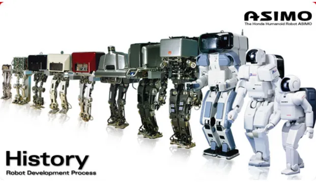
Fig. 1 History of Honda’s humanoid robot ... 2
Fig. 2 ASIMO ... 3
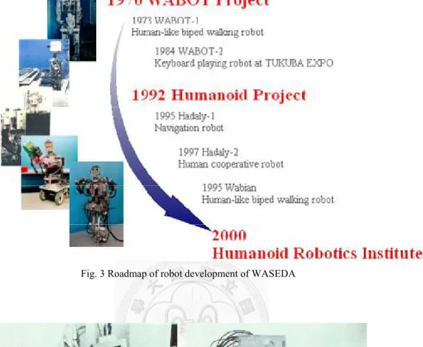
Fig. 3 Roadmap of robot development of WASEDA ... 4
Fig. 4 The history of biped robot in Waseda University. ... 6
Fig. 5 WABIAN-2R ... 7
Fig. 6 DOF configuration of conventional humanoid robot ... 8
Fig. 7 DOF Configuration of WABIAN-2 ... 8
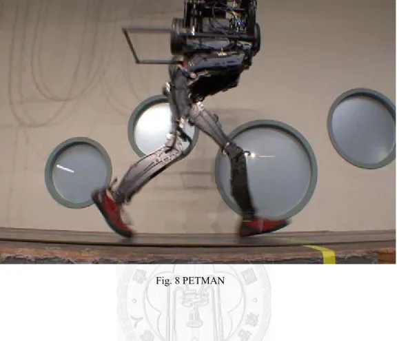
Fig. 8 PETMAN ... 9
Fig. 9 The ground reactive force of foot ... 10
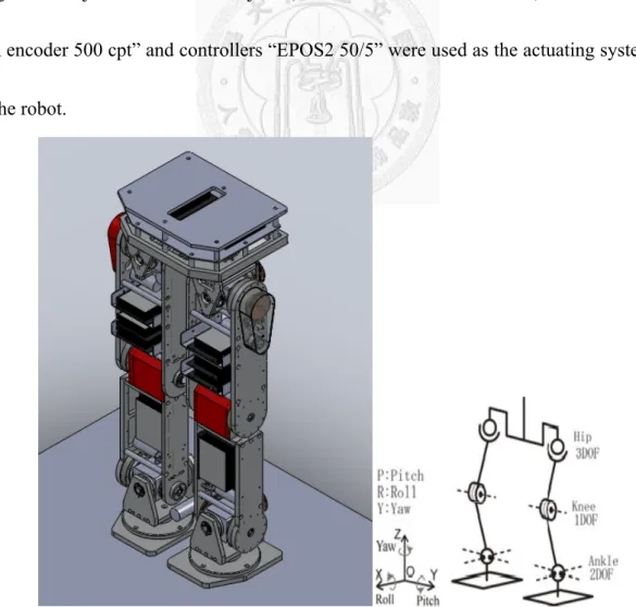
Fig. 10 The 3D CAD model of the biped robot ... 12
Fig. 11 The actual biped robot ... 13
Fig. 12 The Maxon motor and controller ... 14
Fig. 13 First and final CAN device have to connect terminal resistances (120 omegas) ... 15
Fig. 14 Master of the CANOpen and the layout of I/O ports ... 15
Fig. 15 The 6-axis force sensor “IFS-67M25T50- M40BS”... 16
Fig. 16 The structure of using MATLAB and Visual C++ ... 18
Fig. 17 The relationship between two joints in DH coordinate system ... 19
Fig. 18 Control structure of the biped robot. ... 29
Fig. 19 Walking cycle for one step ... 30
Fig. 20. The behavior of human walking ... 33
Fig. 21. The five links model for interpreting. ... 34
Fig. 22. One step of case 1 ... 35
Fig. 23. The free body diagram of the model ... 35
Fig. 24 The concept of potential barrier ... 38
Fig. 25 One step of case 2 ... 40
Fig. 26 Spring Loaded Inverted Pendulum Model ... 40
Fig. 27 Comparing the potential barrier between small step and large step ... 41
Fig. 28 Lower down to decrease potential barrier ... 42
Fig. 29 Implementing “lowering down-rising up” behavior for biped robot ... 43
Fig. 30 Lowering and tuning the position of acme forward would decrease the potential barrier ... 44
Fig. 31 The 2D robot for simulation ... 44
Fig. 32 Simulation for walking algorithm ... 45
XI
Fig. 33 Modeling for inverse pendulum process ... 47
Fig. 34 Free body diagram of the robot’s foot of supporting leg ... 47
Fig. 35 Free body diagram of the inverse pendulum part ... 48
Fig. 36 The two desired postures
θ ( T
d+ T
u)
andθ
(T
d +T
u +T
i). ... 50Fig. 37 The plot of θ(t) versus t with each r. ... 50
Fig. 38 The illustration of stable and unstable positions ... 51
Fig. 39 The robot falls down forward while r=2cm, which is an unstable position. ... 52
Fig. 40 The robot walks stably since we pull r backward from 2cm to -5cm, which is a stable position ... 53
Fig. 41 The whole walking processes ... 53
Fig. 42 Flow char of the tuning process ... 56
Fig. 43 Simulation of the walking pattern with step length: 15cm, step time: 2s, walking velocity: 7.5 cm/s, acme: (3cm, 70.5cm) and r: -8cm. ... 60
Fig. 44Simulation of the walking pattern with step length: 20cm, step time: 1s, walking velocity: 20 cm/s, acme: (5cm, 71cm) and r: -5cm. ... 61
Fig. 45 Simulation of the walking pattern with step length: 30cm, step time: 1s, walking velocity: 30 cm/s, acme: (5cm, 69.5cm) and r: -5cm. ... 62
Fig. 46 Walking experiment with step length: 15cm, step time: 2s, walking velocity: 7.5 cm/s, acme: (3cm, 70.5cm) and r: -8cm. ... 64
Fig. 47 Joint angles of the walking pattern with step length: 15cm, step time: 2s. ... 65
Fig. 48 Block diagram of Adaptive Impedance Control with Gravity Compensation ... 69
List of Tables
Table. 1 Reduction ratio and range of each joint ... 14 Table. 2 D.H. coordinate system of front leg ... 26 Table. 3 D.H. coordinate system of rear leg ... 27
`
1
Chapter 1 INTRDOCTION
1.1 Motivation
In recent years, many countries such as Japan, Korea and USA, have developed a
lot of human size biped robots. These robots have human-like upper and lower limbs,
and they are already used in many fields, such as entertainment, home care and military.
However, although they can mimic many behaviors of humans, they could not perform
naturally like humans, especially on walking. In [1] , for controlling the walking
stability of the robot, the hip trajectory is planned at the same height, so the knees of
the robot would bend while walking. However, this does not make sense when humans
walk.
To deal with the problem, in this thesis, we propose a walking algorithm in which
we can preserve the walking stability of the robot with stretching its knee, to generate
the hip trajectory with different heights.
1.2 Literature Review
1.2.1 ASIMO
ASIMO was created at Honda's Research & Development Wako Fundamental
Technical Research Center in Japan. It is the current model in a line of twelve that
began in 1986 with E0 (Fig. 1).
Fig. 1 History of Honda’s humanoid robot
ASIMO resembles a child in size and is the most human-like robot HONDA has
made so far. The robot has 7 DOF (Degrees of freedom) in each arm — two joints of 3
DOF, shoulder and wrist, giving "Six degrees of freedom" and 1 DOF at the elbow; 6
DOF in each leg — 3 DOF at the crotch, 2 DOF at the ankle and 1 DOF at the knee; and
3 DOF in the neck joint. The hands have 2 DOF — 1 DOF in each thumb and 1 in each
finger. This gives a total of 34 DOF in all joints.
Officially, the name is an acronym for "Advanced Step in Innovative MObility"
( Fig. 2). Honda's official statements indicate that the robot's name is not refer to science
fiction writer and inventor of the Three Laws of Robotics, Isaac Asimov. In Japanese,
the name is pronounced ASIMO and, not coincidentally, means "legs also".
3 Fig. 2 ASIMO
As development continues on ASIMO, today Honda demonstrates ASIMO around
the world to encourage and inspire young students to study the sciences. And in the
future, ASIMO may serve as another set of eyes, ears, hands and legs for all kinds of
people in need. Someday ASIMO might help with important tasks like assisting the
elderly or a person confined to a bed or a wheelchair. ASIMO might also perform
certain tasks that are dangerous to humans, such as fighting fires or cleaning up toxic
spills
1.2.2 WASEDA Series
The other famous institute of studying biped robot in Japan is Humanoid Robotics
Institute in Waseda University. People in the institute developed a lot of robot since the
starting of WABOT Project in 1970, Fig. 3 shows the roadmap of robot development of
WASEDA, while shows the history of the biped robot in Waseda University.
Fig. 3 Roadmap of robot development of WASEDA
(a)WL-1 (b)WL-3
5
(c)WL-5 (d)WABOT-1
(e) WL-9DR (f) WL-10R
(g) WL-10RD (h) WL-12
(i) WABIAN (j) WABIAN-RV Fig. 4 The history of biped robot in Waseda University.
Now, the newest robot in Waseda University is WABIAN-2R (Fig. 5).
7 Fig. 5 WABIAN-2R
WABIAN-2 has been designed accordingly in order to develop a humanoid robot
with the height of 1475 mm, and the weight of 67.5 kg. This robot was developed In
order to mimic the various motions which the human does usually. It consisted of
41-DOFs. (7-DOFs Legs, 2-DOFs Waist, 2-DOFs Trunk, 7-DOF Arms, 3-DOF Hands,
and 3-DOF Neck) Link length and movable range are designed in reference of human
motion measurement in rehabilitation.
The unique feature of WABIAN-2R is the waist mechanism. Conventional biped
humanoid robot has 12 -DOF in the lower limb, and each leg has 6-DOF. Fig. 6 shows
DOF configuration of conventional humanoid robot. This is different from humans who
have more DOF in the lower limb, and therefore have the ability to realize various
walking motions.
Fig. 6 DOF configuration of conventional humanoid robot
Therefore, in order to realize more human-like walking motions, 2-DOF
mechanism (Roll, Yaw) is added to waist part (Fig. 7). This new mechanism has an
advantage which makes this robot easier to walk with stretching knee due to the
independent orientation of trunk movement.
Fig. 7 DOF Configuration of WABIAN-2
9
1.2.3 PETMAN
Fig. 8 PETMAN
PETMAN[5] is an anthropomorphic robot made by Boston Dynamics for testing
chemical protection clothing used by the US Army. Unlike previous suit testers, which
had to be supported mechanically and had a limited repertoire of motion, PETMAN
will balance itself and move freely, such as walking, crawling and doing a variety of
suit-stressing calisthenics during exposure to chemical warfare agents.
PETMAN will also simulate human physiology within the protective suit by
controlling temperature, humidity and sweating when necessary, all to provide realistic
test conditions.
Natural, agile movement is essential for PETMAN to simulate how a soldier stresses
protective clothing under realistic conditions. The robot will have the shape and size of
a standard human, making it the first anthropomorphic robot that moves dynamically
like a real person.
1.2.4 Zero Moment Point
Z.M.P(Zero Moment Point) is a concept related with dynamics and control of
legged locomotion. This concept was introduced in January 1968 by Miomir
Vukobratović and Davor Juričić at The Third All-Union Congress of Theoretical and
Applied Mechanics in Moscow.
From that time, many biped robot based on ZMP concept were developed, and this
concept was spread widely in the field of biped robot.
As shown in Fig. 9, assume that the ground distributive force can be regarded as an equivalent force N , which is acted on the pressure centerp, with a momentM.
Fig. 9 The ground reactive force of foot
11
However, in general, the ground could not provide the momentMfor the foot.
That is, Mneeds to be zero. Therefore, if the loading on the foot changes, Mcould
not change to a proper value to balance the foot. So the equivalent force N would
move to specific a position to compensateM automatically. Therefore, this position
would call Zero Moment Point (ZMP).
1.3 Thesis Organization
This thesis is organized as follows. In Chapter 1, we present the motivation,
objective, and literature review. In Chapter 2, we introduce our hardware and software
structure of the biped robot, which including sensors, actuator, software and coordinate
systems. In Chapter 3, we make an analysis of the stability of the robot. In the walking
cycle, we divided it in to three processes, which are lowering down, rising up and
inverse pendulum process. Lowering down and rising up processes would be combined
as “lowering down-rising up process” to analyze its stability. In Chapter 4, we would
show the simulation result and walking result. Finally, conclusion and main
contributions would be shown in Chapter 5. The Chapter 6 is the future works, which
describes the problems of the actual biped robot of our experiment we encounter but
haven’t solved, and some viewpoints and methods for people who continue to study
the research to refer.
Chapter 2 SYSTEM STRUCTURE OF BIPED ROBOT
2.1 Hardware Structure
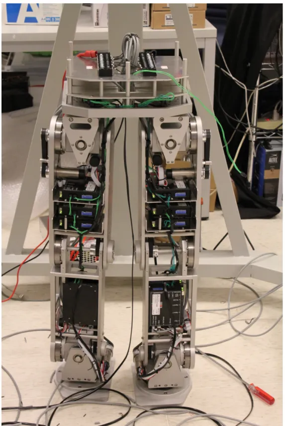
Fig. 10 and Fig. 11 show the 3D CAD model and the actual biped robot, which has
6 degrees of freedom in each leg, and it is 87.6 cm of its height (without trunk), 40 kg
of its weight (without batteries). The reduction gear of each joint is composed of a
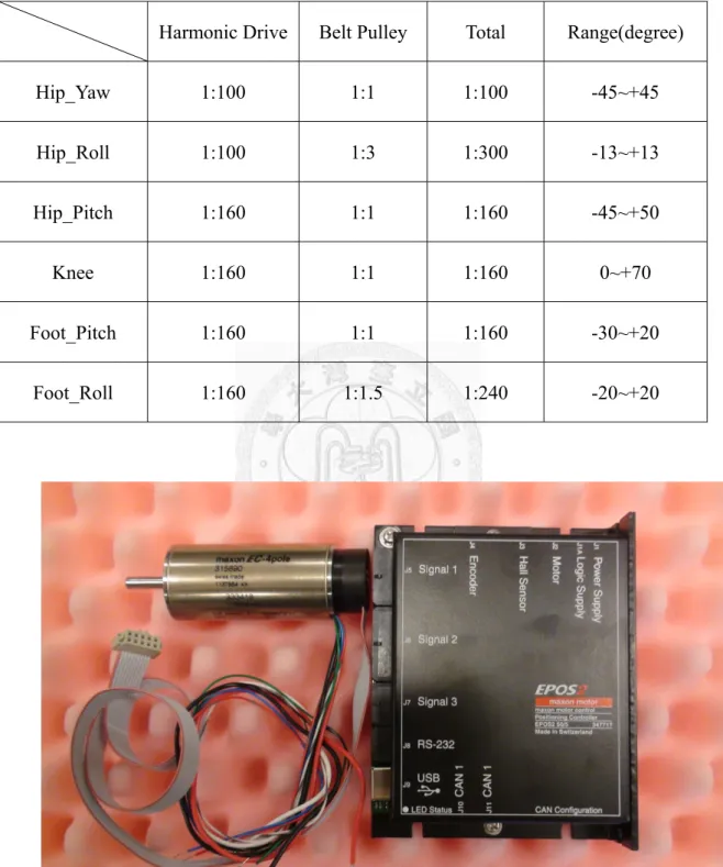
harmonic drive and belt pulley, Table. 1 shows the detail of the reduction ratio and
range of each joint. To drive these joints, Maxon motors “EC-4Pole 30, 200 watt with
MR encoder 500 cpt” and controllers “EPOS2 50/5” were used as the actuating system
of the robot.
Fig. 10 The 3D CAD model of the biped robot
13
Fig. 11 The actual biped robot
Table. 1 Reduction ratio and range of each joint
Harmonic Drive Belt Pulley Total Range(degree)
Hip_Yaw 1:100 1:1 1:100 -45~+45
Hip_Roll 1:100 1:3 1:300 -13~+13
Hip_Pitch 1:160 1:1 1:160 -45~+50
Knee 1:160 1:1 1:160 0~+70
Foot_Pitch 1:160 1:1 1:160 -30~+20
Foot_Roll 1:160 1:1.5 1:240 -20~+20
Fig. 12 The Maxon motor and controller
To make communication between the main computer mounted on the robot and
15
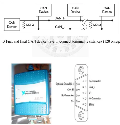
each motor, CANOpen is used here. CANOpen is a high speed communication
protocol, which is very popular in modern industry. As shown in Fig. 13, we have to
connect first and final driver with 120 omega resistor, since the master of the
CANOpen has to know the terminals. The I/O ports of the CANOpen mater is shown
in Fig. 14. We just connect the CAN_H, CAN_L, and ground to the first driver.
Console can use USB surface to connect CANOpen master and communicate each
driver.
Fig. 13 First and final CAN device have to connect terminal resistances (120 omegas)
Fig. 14 Master of the CANOpen and the layout of I/O ports
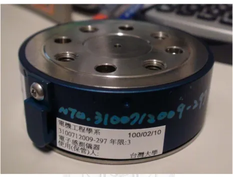
To measure the ground reactive force, the 6-axis force sensor “IFS-67M25T50-
M40BS” is mounted on each foot, which is made by Nitta Corporation. Fig. 15 shows
the sensor.
Fig. 15 The 6-axis force sensor “IFS-67M25T50- M40BS”
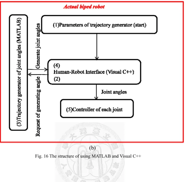
2.2 Software Structure
To control our biped robot, we use MATLAB and Visual C++ and as our main
programs. MATLAB program is used to establish the simulation and compute joint
angles, while Visual C++ program is used to establish the human-robot interface,
which enables us to control the whole motors of the robot. Fig. 16 shows the structure
of using MATLAB and Visual C++.
17
(a)
(b)
Fig. 16 The structure of using MATLAB and Visual C++
In general, to communicate sensors and controllers with the main computer for
the actual robot depends on Visual C++ program, while MATLAB is used as the
computing kernel of the simulation and trajectory generator.
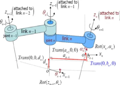
2.3 Robot Coordinate System
In order to determine relationship between posture and each joint of the robot, we
need to establish coordinate system. The most popular coordinate system used in
robotics is the Denavit-Hartenberg convention. In this convention, each homogeneous
transformation that is a 4x4 matrix is represented as a general formula of four basic
19
transformations. The four basic transformations means the four parameters
a
i,α
i,d
i, andθ
i are generally given the names link length, link twist, link offset, and joint angle, respectively. Fig. 17 shows the relationship between two joints in DH coordinate systemFig. 17 The relationship between two joints in DH coordinate system
2.3.1 Robot Forward Kinematic Analysis
The D-H convention allows the construction of the forward kinematics function
by composing the coordinate transformations into one homogeneous transformation
matrix:
1
cos sin cos sin sin cos
sin cos cos cos sin sin
0 sin cos
0 0 0 1
i i i i i i i
i i i i i i i
i i
i i i
a T a
d
θ θ α θ α θ
θ θ α θ α θ
α α
−
−
−
=
(1) .
0 0
0 0 1 2 3 4 5 6 6
6 1 2 3 4 5 6
0 1
R P
T T T T T T T
= =
(2) .
where 0P6 is 3 × 1 transformation vector, 0R6 is 3 × 3 rotation matrix, and 0 is
1 × 3 zero vector.
We will get the relationship between the end-effector and the base coordinate
from Eq.(2). We may summarize the above procedure based on the D-H convention in
the following algorithm for deriving the forward kinematics for any joint robot.
Step l: Locate and label the joint axes z
0….. zn-1.Step 2: Establish the base frame. Set the origin anywhere on the z
0-axis. The x0and y0 axes are chosen conveniently to form a right-hand frame. For i = 1…..n-1,
perform Steps 3 to 5.
Step 3: Locate the origin O
i where the common normal to zi and zi-1 intersects zi. If zi intersects zi-1 locate Oi at this intersection. If zi and zi-1 are parallel, locate Oiin any convenient position along zi.
Step 4: Establish x
i along the common normal between zi-1 and zi through Oi, or in the direction normal to the zi-1–ziplane if zi-1 and zi intersect.Step 5: Establish y
i to complete a right-hand frame.Step 6: Establish the end-effector frame o
nxnynzn. Assuming the n-th joint is revolute, set zn = a along the direction zn-1. Establish the origin on convenientlyalong z , preferably at the center of the gripper or at the tip of any tool that the
21
manipulator may be carrying. Set yn = s in the direction of the gripper closure and
set xn = n as s × a. If the tool is not a simple gripper set xn and yn conveniently to
form a right-hand frame.
Step 7: Create a table of link parameters a
i, di, αi, θi.ai-1 = distance along xi from Oi to the intersection of the zi and zi-1 axes.
di-1 = distance along zn-1 from Oi-1 to the intersection of the xi and xi-1 axes. di-1 is
variable if joint i is prismatic.
αi-1 = the angle between zn-1 and zi measured about xi.
θi-1 = the angle between xi−1 and xi measured about zn−1. θi is variable if joint i is
revolute.
Step 8: Form the homogeneous transformation matrices T
i by substituting the above parameters into Eq. (1).Step 9: Form T
0n = T1…Tn. This then gives the position and orientation of the tool frame expressed in base coordinates.2.3.2 Robot Inverse Kinematic Analysis
The equations we found for solving the inverse kinematic problem of robots can
directly be used to drive the robot to a position. In fact, no robot would actually use the
forward kinematic equations to solve for these results. The equations used are the set of
six (or fewer, depending on the number of joints) equations enable us to calculate the
joint values. In other words, we must calculate the inverse solution and derive these
equations and, in return, use them to drive the robot to position desired.
Equation (3), (4) represent the differential relationship between individual
variables and the function. The Jacobian can be calculated by taking the derivative of
each equation with respect to all variables.
(3) .
(4) .
As we are able to express their position differential change in the joint variation
space Equation (5).
(5) .
Where dx, dy, and dz in [D] represent the differential motion of the hand along the
x-axis, y-axis, and z-axis, respectively, δx, δy, and δz in [D] represent the differential
) , , , ,
(
1 2 3 ji
i
f x x x x
Y =
∂ + ∂
∂ + + ∂
∂
= ∂
∂ + ∂
∂ + + ∂
∂
= ∂
∂ + ∂
∂ + + ∂
∂
= ∂
j j i i
i i
j j
j j
x x x f
x x f
x Y f
x x x f
x x f
x Y f
x x x f
x x f
x Y f
δ δ
δ δ
δ δ
δ δ
δ δ
δ δ
2 2 1
1
2 2 2 1 2
1 2 2
2 1 2 1 1
1 1 1
23
rotations of the hand around the x-axis, y-axis, z-axis, respectively, and represents the
differential motions of the joints. We can divide the differential motion into differential
transformations (translations and rotations).
Differential translations
The frame has moved a differential amount along the three axes. The differential
translations can be represented by Trans (dx, dy, dz).
Differential rotations
A differential rotation is a small rotation of the frame. It is generally represented
by Rot(k, θ).
Differential transformations (translations and rotations)
x x δ δ = sin
1
cos δ x =
(in radians)(6) .
Because the rotation is small, the rotation matrix can be represented:
= −
1 0 0
0
0 1 0
0 1
0
0 0 0
1 ) ,
( x
x x x
Rot δ
δ δ
(7) .
Thus, we assume differential motion with axis k, it is combine with x axis, y axis
and z axis differential motions Equation (5).
+ +
−
− +
− +
−
=
−
−
= −
=
1 0 0
0
0 1
0 1
0 1
1 0 0 0
0 1 0 0
0 0 1
0 0 1
1 0 0 0
0 1 0
0 0 1 0
0 0
1
1 0 0 0
0 1 0
0 1
0
0 0 0 1
) , ( ) , ( ) , ( )
, (
z y x z x y
x z
y x z
y x
y z
z
z y
y x
x
z z Rot y y Rot x x Rot d
k Rot
δ δ δ δ δ δ
δ δ
δ δ δ
δ δ
δ δ
δ δ δ
δ δ
δ
δ δ
δ
θ
(8) .If we neglect all higher order differentials, we get:
−
−
−
=
+ +
−
− +
− +
−
=
=
1 0 0
0
0 1
0 1
0 1
1 0 0
0
0 1
0 1
0 1
) , ( ) , ( ) , ( )
, (
x y
x z
y z z
y x z x y
x z
y x z
y x
y z
z z Rot y y Rot x x Rot d
k Rot
δ δ
δ δ
δ δ
δ δ δ δ δ δ
δ δ
δ δ δ
δ δ
δ δ
δ δ
δ
θ
(9) .And if we want to get differential operator, we can combine differential
translations, differential rotation and subtracting the unit matrix as following:
I d
k Rot dz
dy dx
Trans × −
=
Δ ( , , ) ( , θ )
−
−
−
−
=
1 0 0 0
0 1 0 0
0 0 1 0
0 0 0 1
1 0 0
0
0 1
0 1
0 1
1 0 0 0
1 0 0
0 1 0
0 0 1
x y
x z
y z dz
dy dx
δ δ
δ δ
δ δ
−
−
−
=
0 0 0
0
0 0
0
dz x
y
dy x z
dx y z δ δ
δ δ
δ δ
(10) .
The Jacobian of the robot will create the link between the joint movements and
the hand movement; we can use the calculation of the Jacobian as follows:
25
[ ] [ ][ ] D = J D
θ (11) .] ][
][
[ ] ][
[ J
−1D = J
−1J D
θ (12) .] ][
[ ]
[ D
θ= J
−1D
(13) .Finally, the discrete form of the general solution provided by inverse kinematics is:
z J J I x
J Δ + − Δ
=
Δ θ
+(
+)
(14) .Where
Δ θ
is the unknown vector in the joint variation space,Δx
is variation of one or more end effectors position and orientation in Cartesian space, J+ is the uniquepseudo-inverse of J providing the minimum norm solution, and
Δ
z describes asecondary behavior in the joint variation space.
2.3.3 Trajectory Generator
To establish the trajectory generator, we use the Robotics Toolbox in MATLAB,
which is a powerful toolbox that can help us to compute the kinematics of multi- D.O.F.
system as long as we construct the D.H. coordinate system of the robot for it.
Here, we construct two D.H. coordinate systems of the robot. One is for the front
leg, while the other is for the rear leg, respectively. Table. 2 and Table. 3 show the D.H.
coordinate systems of the robot.
Table. 2 D.H. coordinate system of front leg
α
(rad)a
(cm)θ
(rad)d
(cm)θ
init(rad)1
π2 11.5θ
1 0 π22
π2 0θ
2 10π
3
0 -30θ
3 0 04
0 -30θ
4 0 05
π2 0θ
5 0π
6
0 0θ
6 0 027
Table. 3 D.H. coordinate system of rear leg
α
(rad)a
(cm)θ
(rad)d
(cm)θ
init(rad)1
π2 0θ
1 0π
2
0 30θ
2 0 03
0 30θ
3 0 04
π2 0θ
4 0π
5
0 -11.5θ
5 -10 0To generate joint trajectory, we have to establish the trajectory generator.
Therefore, we use the following steps to establish it:
1. Plan the hip trajectory at pitch direction based on our algorithm in Chapter 3
in 2D Cartesian (planar) space.
2. Use the geometric method to solve planar inverse kinematics to get the pitch
joints of the front leg.
3. Plane Roll joints of the front leg.
4. Use joint angles of the front leg with its D.H. coordinate (Table. 2) to calculate
forward kinematics to get actual position vector of hip trajectory in 3D
cartesian space.
5. Plane position vector of the foot trajectory of rear leg in 3D cartesian space.
6. Subtract the position vector of hip trajectory from the Planed position
vector of the foot trajectory of rear leg to get the position vector relative to
hip.
7. Solve inverse kinematics with the D.H. coordinate of rear leg (Table. 3) to get
each joint angle of rear leg.
Following the above steps, we can generate all joint angles of the robot, and then feed
them to each joint controller through CANOpen to realize stable walking. Fig. 18
shows the control structure of the biped robot.
29
Fig. 18 Control structure of the biped robot.
Chapter 3 WALKING STABILITY ANALYSIS
3.1 Walking Cycle
Fig. 19 Walking cycle for one step
In general, biped walking is a periodic cycle, and it always consists of two phases:
the double support phase and the single support phase. Here, we divide the walking
behavior into three processes: the lowering down process, the rising up process and the
inverse pendulum process, respectively. The lowering down process occurs in double
support phase while the rising up process and the inverse pendulum process happen in
single support phase. Fig. 19 shows the relationship between walking phases and
31
processes of walking behavior.
As we can see in Fig. 19, the lowering down process occurs during
t
=0~T
d. In theprocess, the front leg and the rear leg will cooperate to finish the lower down motion.
When time reaches to
T
d, the lowering down process will end while rising up processwill start. In rising up process, the front leg will stretch to raise the robot while the rear
leg will rise and swing from back to front. Then when time reaches to
T
d+ T
u, the walking behavior would enter the inverse pendulum process. In this process, the kneejoint of supporting leg will be locked, and the ankle joint would swing the robot
forward to prevent it fall down forward. When time reaches to
T
d+ T
u+ T
i, the swing leg will touch the ground, and the total posture will be finished. Therefore, one walkingcycle would be finished, and then next cycle will be started.
In the following topics, we will focus on the stability of these walking processes.
The lowering down and rising up processes would be combined into “lowering
down-rising up process”, and then discussed in Chapter 3.2, while “inverse pendulum
process” will be analyzed in Chapter 3.3. We would use different degrees to analyze
the two processes. That is, different models would be used in different processes.
The main propose in “lowering down-rising up process” is to prevent the robot
fall down backward since its COG (center of gravity) is close to the rear edge of the
supporting leg when it goes from double support phase to single support phase, while
we should prevent it fall down forward in “inverse pendulum process” since it is close
to the front edge of the supporting leg.
3.2 Stable Criteria with Energy Function for Lowering Down-Rising Up Process
In this process, we would imitate the human walking behavior. Observing from our
walking behaviors, when we walk with the same pattern, the knee joint of the front leg
would be locked all the time. However, if we want to accelerate our walking speed, we
might change our walking pattern from the small step to the large step. In this situation,
we would bend our knee joint of the front leg to lower down our center of mass
naturally. Fig. 20 shows the behavior of human walking.
(a) Walking with the same pattern
33
(b) Walking with changed patterns from the small one to the large one by bending our knee Fig. 20. The behavior of human walking
3.2.1 Modeling for Interpreting Human Walking Behavior
Here, our objective is to figure out these natural walking behaviors, and to extract
some useful information for our robot. Before we interpret these behaviors, we would
make some assumptions to the humanoid model as follows, which would make us
easier to figure out them:
(1) We neglect the foot of the model, so that the five links model would be used
here.
(2) We assume the center of mass of the model is located at its hip.
(3) The time table of one step period is defined as follows (DSP means Double
Support Phase, while SSP means Single Support Phase.):
The model can be seen in Fig. 21, we would interpret the above two cases individually.
Fig. 21. The five links model for interpreting.
3.2.2 Case 1: Walking with the same pattern
When we walk with the same pattern, we usually lock the knee joint of the front
leg in one walking period, such as Fig. 22.
35
Fig. 22. One step of case 1
The model would rotate point
O
while walking. Therefore, pointO
is the fulcrum of the walking motion, and the free body diagram can be regarded as Fig. 23.Fig. 23. The free body diagram of the model
According to the Principle of Work and Energy, the change of mechanical energy
equals to the work done by all non-conservative forces. In our model, there exist two
non-conservative forces, which are
F
r( τ )
and
F
f( τ )
, respectively, and
F
f( τ )
does not do any work since it pass the fulcrum
O
. Therefore, we can write the mechanical energy function during one step as follows: × ⋅
+
= ( )
(( ) )[ ( ) ( )] ( )
)
(
tt r r
Dstart me
me Dstart
d F
r t
E t
E
θθ
τ τ θ τ
( 15 )
Where
E
me( t
Dstart)
is the initial mechanical energy of one step, andSend
Dstart
t t
t ≤ <
. The term
((t) )[ ( ) × ( )] ⋅ ( )
t r r
Dstart
d F
θ
r
θ
τ τ θ τ
means the work
done by the ground reactive force of the rear leg
F
r( τ )
, and we need to notice that
) ( τ F
ris only available in DSP, such as Eq.(16).
Send Sstart
Sstart Dstart
r
t t
t for t
F f
<
≤
<
≤
=
τ τ τ τ
0 ) ) (
(
( 16 )
0 ) ( τ >
f where
The rear leg can only do work in DSP, and the work must be a non-negative value
since the term
r
r( τ ) F
r( τ )
×
has the same direction asd θ ( τ )
while walking forward. Eq.(17) shows the relationship of work in different time segment.
<
≤
<
≤
=
⋅
×
≥
⋅
×
Send Sstart
Sstart Dstart
r r
r r
t t
t for t
d F
r
d F
r
τ τ τ
θ τ
τ
τ θ τ
τ
0 ) ( )]
( )
( [
0 ) ( )]
( )
(
[
( 17 )
However, the mechanical energy
E
me(t )
must be periodic for every step while periodic walking. Accordingly, the term[ r
r( τ ) × F
r( τ )] ⋅ d θ ( τ )
must be zero for any time; Otherwise,E
me(t )
would not be periodic, and it will go to infinity when37
∞
→
t
since there does not exist any term which can dissipate the energy in Eq.(15).Moreover, since the two terms
r
r( τ ) F
r( τ )
×
andd θ ( τ )
have the same directionand
d θ ( τ )
would not be zero while walking forward, we can ascertain that) ( )
( τ
rτ
r
F
r
×
must be zero, which means thatF
r( τ )
has no normal component.
Therefore, without normal force, friction force would be zero, so the tangential
component of
F
r( τ )
must be zero since it is friction force. That is to say,
F
r( τ )
is zero for any time, so we can guarantee that the duration of DSP (
t
Dstart ≤τ
<t
Sstart)would approach to zero from Eq.(16), which implies that in theory, when we walk with
periodic pattern, only SSP is available. Therefore, Eq.(15) can be simplify into Eq.(18).
Send Dstart
Dstart me
me
t E t for t t t
E ( ) = ( ) ≤ <
( 18 )
Eq.(18) describes that when we walk with periodic pattern, “conservation of
mechanical energy” is used for any time.
In sum, when we walk with periodic pattern, the mechanical energy is conserved
for any time, and only SSP is available in theory. However, in actual situation, there are
some buffering elements in our body structure, such as gristles and foot arch, which is
like the shock absorbers to absorb the vibration while walking, but they also dissipate a
little mechanical energy of our body which is used for walking. Consequently, we need
to supply a little mechanical energy which is dissipated by the buffering elements
every step. So the term
((t) )[ ( ) × ( )] ⋅ ( )
t r r
Dstart
d F
θ
r
θ
τ τ θ τ
would not be zero, and
therefore SSP would have a small duration. Note that the little supplying mechanical
energy is converted from the chemical energy of our body, which means we only need
to spend a little energy stored in our body to maintain the periodic walking every step.
Note that the above walking behavior of the model should accord with the
following assumption:
mgH t
E
me( ) ≥
( 19 )
Otherwise, the model would fall down backward. Therefore, from the inspiration, we
can define a parameter
U
bas follows, which is call potential barrier:The potential barrier
U
bof a trajectory Traj .( , r
g)
θ is the potential energy of the center of mass that passes through the vertical position θ = 0
along the trajectory.
Fig. 24 shows the concept of potential barrier.
Fig. 24 The concept of potential barrier
39
We can also define the stable criteria of walking forward:
Assume the mechanical energy
E
me(t ) of the center of mass of the model is conserved along Traj .( , r
g)
θ during t
Dstart≤ t < t
Sendof one step, and
) (t E
meshould larger or at least equal to
U
b; Otherwise, the model would fall down backward.
That is, the stable criteria of walking forward written in mathematic form would be
that:
E
me( t ) ≥ U
b
( 20 )
We would use this criterion to explain the following case.
3.2.3 Case 2: Walking with changed patterns from small one to large one
When we want to accelerate our walking speed by enlarging our walking pattern
from the small step to the large step, from our observation, we would tend to bend our
knee joint of the front leg to lower down our center of mass naturally, and then rise up
to the original height, such as Fig. 25.
Fig. 25 One step of case 2
To illustrate this phenomenon, let us assume that we would preserve the mechanical
energy from the previous (small) step in the large step. That is, there is no more
mechanical energy converted from the chemical energy stored in our body because of
changing step from smaller one to larger one. In fact, to preserve the mechanical
energy, we can consider the model is like SLIP (Spring Loaded Inverted Pendulum)
model [10] [11] [12] . In the model, the whole body would be simplified into a particle,
and the legs would be considered as a spring to restore the mechanical energy, such as
Fig. 26.
Fig. 26 Spring Loaded Inverted Pendulum Model
41
However, if we still want to lock our knee of front leg for large step, we would
find that the potential barrier of large step is larger than small step, such as Fig. 27.
Fig. 27 Comparing the potential barrier between small step and large step
To finish the walking process, the mechanical energy preserved from the previous
(small) step should accord with Eq.(20). However, from our assumption, it is the same
as the small step. That is to say, from the degree of mathematics, we cannot ensure that
it would accord with Eq.(20) since the potential barrier become larger in large step.
Nevertheless, we have the sense of our own mechanical energy of our body and the
potential barrier of the step we walked. We would first predict whether we can accord
with Eq.(20) with locking the knee of front leg or not. If we predict that it would work,
we would still walk with locking our knee of front leg, which is like in Case 1.
Otherwise, we will bend the knee of the front leg to lower down our center of mass to
decrease potential barrier, and then rise up to the original height such as Fig. 28 .
Fig. 28 Lower down to decrease potential barrier
Therefore, according to our explanation in theory, if we want to implement
human-like walking on a biped robot, we can preset the mechanical energy of the
center of mass of the robot, which would be preserved at the same value for all
walking process, of course, it should accord with Eq.(20) of the trajectory of center of
mass we plan. Then the robot would be able to walk.
However, there exist modeling errors between the model and actual biped robot
such that we assume its center of mass is concentrated at its hip. That is, we cannot get
the exact mechanical energy through the model, so we cannot ensure it would accord
with Eq.(20).
Nevertheless, our explanation also imply that if we cannot ensure whether the
mechanical energy is larger than the potential barrier, “lowering down-rising up”
would be the conservative way for walking since it can decrease the potential barrier.
43
Therefore, to consider the problem, we would not follow the theoretical method totally,
but keep the “lowering down-rising up” behavior.
3.2.4 Implementing Lowering Down-Rising Up Behavior for a Biped Robot
To implement “lowering down-rising up” behavior for a biped robot, we only need
to choose three positions, which are initial position, end position and acme, and using
spline curves to connect each other. By tuning the acme, we can get several trajectories
with different potential barriers for center of mass. Fig. 29 shows this method.
Fig. 29 Implementing “lowering down-rising up” behavior for biped robot
For tuning the position of acme, there is a useful tip that if the robot fall down
backward, lowering and tuning the position of acme forward would amend the
situation since this way would help the robot to decrease the potential barrier. Fig. 30
shows our description.
Fig. 30 Lowering and tuning the position of acme forward would decrease the potential barrier
In [13], we build a 2D robot for simulation to demonstrate this walking algorithm
(Fig. 31). We use strait line to connect initial position, acme and end position to
generate several trajectories, and then we use Simulated Annealing with one step time
interval as its cost function to help us to select a stable trajectory for the robot. Fig. 32
shows the simulation result.
Fig. 31 The 2D robot for simulation
45
(a) (b)
(c) (d)
(e) (f)
(g) (h) Fig. 32 Simulation for walking algorithm
3.3 Stable Criteria with ZMP for Inverse Pendulum Process
By tuning the acme position in lowering down-rising up process, we have our robot
overcome the potential barrier, which would enable our robot to have human-like
walking and prevent it falling down backward. However, that process could not ensure
the robot not to fall down forward. Consequently, to prevent the robot from falling
down forward, ZMP concept would be used in inverse pendulum process. In this
process, we would generate the stable hip trajectory by keeping the position of ZMP,
r
in the foot polygon.3.3.1 Modeling for Inverse Pendulum Process
In this process, we would make some assumptions as follows:
(1) The whole mass of the robot is concentrated on its hip donated as
m
, and it is supported by the foot of the supporting leg, which is in static equilibrium,and the knee joint of the supporting leg do not rotate during inverse
pendulum process for keeping
L
to be constant.(2) For convenient to solve the dynamic equation, we assume
θ
is small, and the mass center does not move drastically at vertical direction. Therefore, wewould neglect its nonlinear terms. i.e. vertical acceleration
a
y≅ 0
,θ θ ≅
sin
,cos θ ≅ 1
,θ
2≅ 0
.47
Fig. 33 Modeling for inverse pendulum process
3.3.2 Derivation for Hip Trajectory
To derive the hip trajectory of the robot, we first take the free body diagram of its
foot of supporting leg to get Eq.(21):
Fig. 34 Free body diagram of the robot’s foot of supporting leg
0 ) (
) (
) (
0 − − + − + − =
Mp = F
yr M F
x f
y x
F f F
r = M +
( 21 )
Where