黎曼曲面與橢圓函數的理論及其對正弦高登方程的應用

應 用 數 學 系

碩 士 論 文

黎曼曲面與橢圓函數的理論

及其對正弦高登方程的應用

The Theories of

Riemann Surfaces and Elliptic Functions

with Application to the sine-Gordon Equation

　研究生：陳建澤 　　

指導教授：李榮耀 教授

及其對正弦高登方程的應用

The Theories of

Riemann Surfaces and Elliptic Functions

with Application to the sine-Gordon Equation

　研究生：陳建澤 　　

Student: Jian-Ze Chen

指導教授：李榮耀 教授

Advisor: Jong-Eao Lee

國 立 交 通 大 學

應 用 數 學 系

碩 士 論 文

A Thesis

Submitted to Department of Applied Mathematics

College of Science

National Chiao Tung University

In Partial Fulfillment of the Requirements

for the Degree of Master

in

Applied Mathematics

June, 2013

及其對正弦高登方程的應用

　研究生：陳建澤 　　

指導教授：李榮耀 教授

國 立 交 通 大 學

應 用 數 學 系

摘要

中華民國 一０二 年 六 月

Riemann Surfaces and Elliptic Functions

with Application to the sine-Gordon Equation

Student: Jian-Ze Chen

Advisor: Jong-Eao Lee

Department of Applied Mathematics

National Chiao Tung University

Abstract

The Goal of this paper is to solve the sine-Gordon equation,

utt− uxx+ sin[u(x, t)] = 0, where − ∞ < x < ∞ and t > 0. By using the method of substitution, we get

uss+ sin[u(s)] = 0,

which is a simple pendulum motion at time s with the angular displacement u, and it implies us=

√

2[E + cos(u)], where E is constant.

But √2[E + cos(u)] is a two-valued function on C, so we introduce the theory of the Riemann surface R such that it comes to a single-valued analytic function on this surface.

在整篇論文的研究中，非常感謝指導教授李榮耀 老師。老師在給我們方向之後， 給我們很大的空間去研究與發揮，對於我們的問題也會親切地解惑，並鼓勵我們學生 互相協助與討論。回想研究的一年，過程與回憶是有收穫的，非常感謝。 在努力的過程中，同伴的協助對於我的研究，是非常重要的。感謝同一間研究 室的范名宏，給我極大的鼓勵與協助，毫不保留地幫助我、聽我抱怨，非常感恩；感 謝蔣宜津，這一路上我們時常在討論研究中所遇到的許多疑惑跟難題，在討論的過程 中，我們都領悟了許多學術分析上的技巧，很謝謝妳這一年來的協助。 當然也要感謝我的父母陳協成、黃美芬，研究最後的這一年，我幾乎都待在新 竹，沒有辦法時常回去陪伴您們，也謝謝您們的包容與鼓勵。 最後我要感謝無時無刻都陪伴我的黃政運，不管我在學校研究到多晚，你都願意 來載我回去，就算我半夜還在用電腦寫論文，可能打擾到你的睡眠，你依然包容我、為 我加油。這一年，我的成就，多虧有你，謝謝你。 最後謝謝我所有親朋好友的陪伴，感恩。

1 Introduction 1

2 The Riemann Surfaces of Genus N 3

2.1 The Geometric Structure . . . 4 2.2 The Algebraic Structure . . . 10 2.3 The Paths on the Riemann Surfaces of Genus N with Algebraic Structures 14 2.4 The Path Integrals on Riemann Surfaces . . . 16

3 The Pendulum Motion on Riemann Surface 43

4 The Elliptic Functions 55

4.1 Definition and Properties of Elliptic Functions . . . 55 4.2 The Theta-Functions . . . 56 4.3 The Jacobian Elliptic Functions . . . 59

5 The sine-Gordon Equation 61

5.1 The Special Solutions of the sine-Gordon Equation . . . 61 5.2 The Periods of Those Solutions . . . 66

6 Conclusion 69

Appendix I

A The Integrals over a, b-cycles I

A.1 a1-cycle . . . I

A.2 a2-cycle . . . II

A.3 a3-cycle . . . III

A.4 b3-cycle . . . IV

A.5 b2-cycle . . . V

References IX

2.1 f (z) =√z . . . . 3

2.2 Sheet-I and sheet-II . . . 4

2.3 Complex planes and the corresponding Riemann spheres . . . 5

2.4 Separating the edges of cuts on the spheres . . . 5

2.5 Opening of the hemipheres face each other . . . 6

2.6 Riemann surface R of genus 0 . . . 6

2.7 R with branch point z1 . . . 7

2.8 Cut plane and the corresponding branch cuts . . . 7

2.9 Complex plane and the corresponding Riemann sphere . . . 8

2.10 Opening of the hemipheres face each other . . . 9

2.11 Riemann surface R of genus m_{− 1 . . . .} 9

2.12 Deffrence of the same path in sheet-I and sheet-II . . . 10

2.13 Example 2.1, the path in _{C and the corresponding path in R . . . 10}

2.14 Example 2.2, the path in C and the corresponding path in R . . . 11

2.15 Example 2.3, the path in _{C and the corresponding path in R . . . 11}

2.16 Path for case of the different branch points . . . 12

2.17 Path inC and the corresponding path in R, with the branch points 0 . . . 12

2.18 Path in_{C and the corresponding path in R, with the branch points z}1 . . 13

2.19 Path for case of the different branch cuts . . . 13

2.20 Path in_{C and the corresponding path in R, with the cut of first kind . . . 14}

2.21 Path inC and the corresponding path in R, with the cut of second kind . 14 2.22 Example 2.4, the cycles ai inC and the corresponding cycles in R . . . 15

2.23 Example 2.5, the cycles bi in C and the corresponding cycles in R . . . 15

2.24 Cycle a crossover a cut . . . 17

2.25 Cycle a = a1 ∪ a2 crossover a cut and some auxiliary paths . . . 17

2.26 Cycle a and the equivalent paths r1 and r2 . . . 18

2.27 Cycle b crossover two cuts . . . 19

2.29 Cycle b and the equivalent paths r1 and r2 . . . 20

2.30 Paths r1 and r2 for Pro. 2.1 . . . 21

2.31 Paths r1 and r2 for Pro. 2.2 . . . 22

2.32 Cut with end point z1 . . . 24

2.33 Modified-Value Domain for the cut with end point z1 . . . 25

2.34 Cut with end points z1 and z2 . . . 25

2.35 S+_{, S}−_{, T}+_{, and T}− _{. . . 27}

2.36 S−∩ T+ _{. . . 27}

2.37 Cut with end point z1 . . . 28

2.38 Cut with end points z1 and z2 . . . 29

2.39 Branch points and the branch cuts of f (z) . . . 31

2.40 Cycle c1 and the equivalent paths c11 and c12 . . . 32

2.41 Cycle c2 and the equivalent paths c21, c22, c23, and c24 . . . 34

2.42 Cycle d1 and the equivalent paths d11, d12, d13, and d14 . . . 36

2.43 Cycle d2 and the equivalent paths d∗1, c12, d21, d22, d23, d24, and d25 . . . . 39

3.1 Branch points and the branch cuts of us . . . 45

3.2 a-cycles . . . . . . . 46

3.3 The equivalent paths of a1-cycle . . . 47

3.4 The equivalent paths of a2-cycle . . . 48

3.5 The equivalent paths of a3-cycle . . . 49

3.6 b-cycles . . . 50

3.7 The equivalent paths of b3-cycle . . . 51

3.8 The equivalent paths of b2-cycle . . . 52

Introduction

The Goal of this paper is to solve a second-order partial differential equation, that of the sine-Gordon equation [1].

The sine-Gordon equation is

utt− uxx+ sin[u(x, t)] = 0, where − ∞ < x < ∞ and t > 0, and by letting s = αx_{− βt with β}2_{− α}2 _{= 1, the original equation comes to}

uss+ sin[u(s)] = 0.

We multiply an intergral factor us on both sides, and integral it with respect to s, we get 1

2u

2

s − cos (u) = E, where E is constant, then us =± √

2[E + cos(u)].

Assume without loss of generality that us = √2[E + cos(u)], it is a two-valued function on complex plane_{C, so we introduce the theory of the Riemann surface R such} that √2[E + cos(u)] is a single-valued analytic function on this surface [2].

Next, we discuss the situations of the modified value in the MATHEMATICA on the Riemann surface R [3][4], so that we can use this skill to solve us =

√

2[E + cos(u)] by approximation of cos(u) by the Taylor series at 0.

We back to consider us=

du

ds =

√

2[E + cos(u)], we get

s =

∫ u(s)

0

1 √

2[E + cos(U )]dU,

and in order to solve it, we introduce the classical theory of the elliptic functions [5]. The theory occurs on Riemann surfaces of genus 1.

Finally, we use this theory to find out the special solutions and the corresponding periods of above integral problem on Riemann surfaces of genus 1.

The Riemann Surfaces of Genus N

To begin with, we have z∈ C, and by using the polar form,

z =|z|(cos θ + i sin θ)

=|z|eiθ, for some θ, where e is an Euler’s number.

Now, let f (z) =√z, and notice that z =|z|eiθ ₌|z|ei(θ+2nπ)_, ∀n ∈ Z, then

f (z) =√z =|z|12ei θ+2nπ 2 = { |z|1 2ei θ 2 if n is even, −|z|1 2ei θ 2 if n is odd. Fig. 2.1 f (z) =√z

Thus, f (x) is a two-valued function, so we want to let f (x) become a single-valued function. Now, we will modify its domain C to construct the corresponding new surface,

2.1 The Geometric Structure

Consider some nonzero complex number z0 =|z0|eiα, for some α, we have

f (z0) = √ z0 =|z0| 1 2ei α 2.

Fixing _|z0|, and if α increases by 2π, f(z0) comes to the value |z0|

1 2ei α+2π 2 = −|z0| 1 2ei α

2, which is precisely the negative of its original value. Continuing above way,

then α increases by 2π, f (z0) comes to its original value.

In this sense, we cut the extended complex plane along the line, reiα_{, for all} non-negative r ∈ R, and restrict the angle, we get two single-valued branches of f(z):

{ f (z) =|z|12ei θ 2, θ ∈ [α − 2π, α), f (z) =|z|12ei θ 2, θ ∈ [α, α + 2π).

Now, we take these two cut planes of the complex plane, and call them sheet-I and

sheet-II , and call the cut a branch cut.

Notice that, the cut on each sheet has two edges, we label the starting edge with a +, and label the ending edge with a −. Then attach the + edge of the cut on one of these two sheets, to the_{− edge of the cut on the other. Thus, whenever we cross the cut,} we pass from one sheet to the other.

This two-sheeted surface we cannot be realized in three-dimensional Euclidean space, so we want to build a new surface.

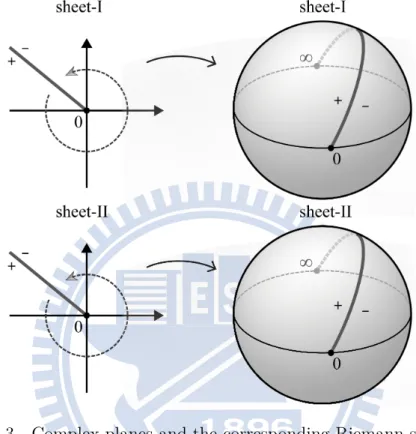
To begin with, we use the stereographic projection, the two sheets to be the Rie-mann spheres (Fig. 2.3).

Fig. 2.3 Complex planes and the corresponding Riemann spheres

Furthermore, we pretend that the spheres are made of rubber, we separate the edges of cuts (Fig. 2.4).

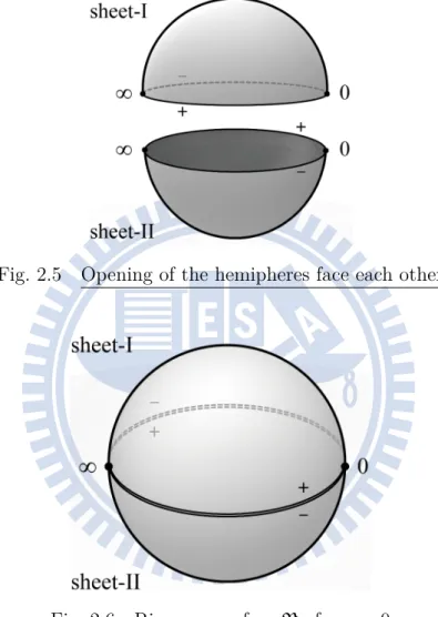
Finally, we deform each sheet into a hemisphere, and rotated each sheet so that the opening of the hemipheres face each other (Fig. 2.5), and paste the edges marked + and

− each other. Therefore, we glue the two hemishperes together to be a sphere and call it

a Riemann surface R of genus 0 (Fig. 2.6).

Fig. 2.5 Opening of the hemipheres face each other

Fig. 2.6 Riemann surface R of genus 0

Notice that, in this new surface R, the + edge of sheet-I is equivalent to the_{− edge} of sheet-II, and the _{− edge of sheet-II is equivalent to the + edge of sheet-I.}

Since f (z) =√z =√z− 0, we call 0 a branch point.

Consider the different branch point z1, in the manner of f (z) =

√

z, we also have

the Riemann surface R of genus 0 (Fig. 2.7).

Fig. 2.7 R with branch point z1

Before we discuss the general case of the construction of R, consider the following situation.

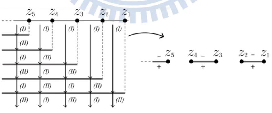
We consider f (z) =√∏(z− zk) for distinct zk ∈ C, all arguments of zk are same, and |z1| < |z2| < . . . < |zn|, i.e., for all zk on the same line orderly.

Now, we cut plane start from zk to∞ along this line. Recall that we pass to another sheet when we cross the cut, and so f (z) is precisely the negative of its original value. Therefore, if the path cross even cuts, we pass to the same sheet, that is, there’s no branch cut; on the contrary, if the path cross odd cuts, there’s a branch cut (Fig. 2.8).

Now, we consider the general case, f (z) = v u u t∏n k=1 (z− zk) =√(z− z1) √ (z− z2) . . . √ (z− zn), where zk are distinct branch points, then we have m branch cuts:

{

1. z1z2, z3z4, . . . , z2m−1z2m, if n = 2m,

2. z1z2, z3z4, . . . , z2m−1 → ∞, if n = 2m − 1.

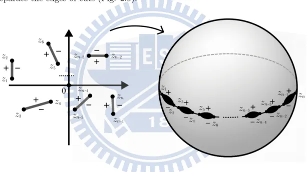
In like manner, there are two sheets and the corresponding Riemann spheres, and we separate the edges of cuts (Fig. 2.9).

Fig. 2.9 Complex plane and the corresponding Riemann sphere

Finally, we deform and rorate each sheet so that the opening of them face each other (Fig. 2.10), and paste the edges marked + and − each other. Therefore, we glue them together to be a Riemann surface R of genus m− 1, that is, m − 1 holes (Fig. 2.11).

Fig. 2.10 Opening of the hemipheres face each other

Fig. 2.11 Riemann surface R of genus m− 1

Notice that, in this case, if f (z) has 2m or 2m_{−1 branch points, we have m branch} cuts, and construct the Riemann surface R of genus m_{− 1.}

2.2 The Algebraic Structure

Now, in order to distinguish which sheet a path belongs when this path in the complex plane, we define that the path in the sheet-I is solid line, and the path in the sheet-II is dash line.

Fig. 2.12 Deffrence of the same path in sheet-I and sheet-II

The followings are some examples of those paths inC and the corresponding paths in R.

Example 2.1. The path is start from point A on the + edge in the sheet-I, to point B

on the _{− edge in the sheet-I, and cross the cut to point C on the − edge in the sheet-II,} shown in Fig. 2.13.

Example 2.2. The path is start from point A in the sheet-I, to point B on the _{− edge in}

the sheet-I, and cross the cut to point C in the sheet-II, shown in Fig. 2.14.

Fig. 2.14 Example 2.2, the path inC and the corresponding path in R

Example 2.3. The path is start from point A in the sheet-I, to point B on the + edge in

the sheet-I, and cross the cut to point C in the sheet-II, shown in Fig. 2.15.

The followings are the different situations of same path in _{C with the different} branch points.

We consider the path is start from point A to point B, shown in Fig. 2.16.

Fig. 2.16 Path for case of the different branch points

Then, we consider the branch points 0 and z1, we get the different corresponding

paths in R, shown in Fig. 2.17 and 2.18.

Fig. 2.18 Path in_{C and the corresponding path in R, with the branch points z}1

And, the followings are the different situations of same path inC with the different branch cuts.

We consider the path is start from point A to point B, shown in Fig. 2.19.

Fig. 2.19 Path for case of the different branch cuts

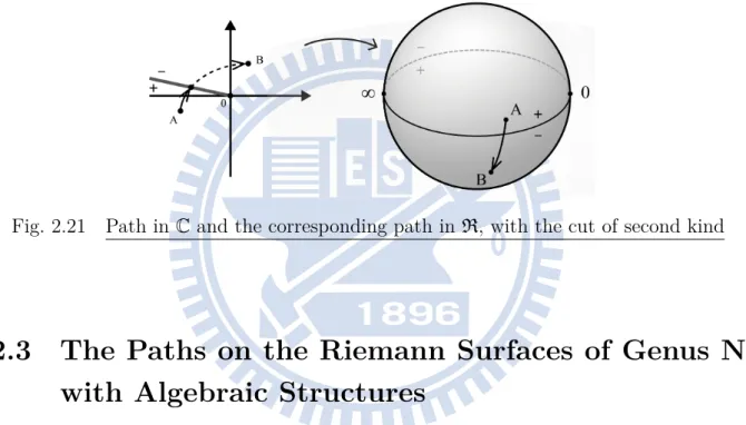
Then, we consider the different branch cuts, we get the different corresponding paths in R, shown in Fig. 2.20 and 2.21.

Fig. 2.20 Path in_{C and the corresponding path in R, with the cut of first kind}

Fig. 2.21 Path in C and the corresponding path in R, with the cut of second kind

2.3

The Paths on the Riemann Surfaces of Genus N

with Algebraic Structures

Notice that, by the Cauchy integral formula, for any closed path in R of genus m is homotopic to an integral linear combination of the loop-cuts ai and bi, i = 1, 2, . . . , m, so we will consider the integrals of f (z) over a, b-cycles, in this paper, help us to obtain the integrals.

The followings are some examples of a, b-cycles in _{C and the corresponding cycles} in R. Example 2.4. Consider f (z) = v u u t∏5 k=1 (u− uk), shown in Fig. 2.22.

And, we consider the cycles a1 and a2 in C, and the corresponding cycles in R of

genus 2.

Fig. 2.22 Example 2.4, the cycles ai inC and the corresponding cycles in R

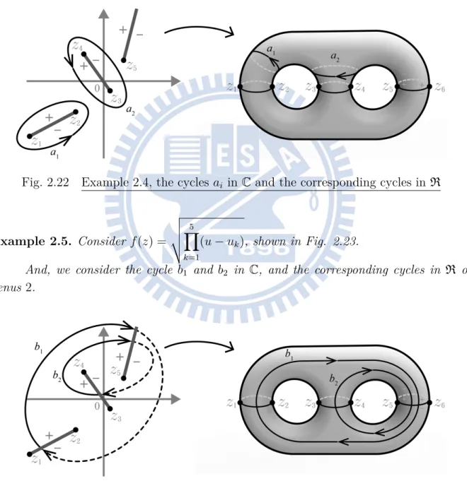
Example 2.5. Consider f (z) = v u u t∏5 k=1 (u− uk), shown in Fig. 2.23.

And, we consider the cycle b1 and b2 in C, and the corresponding cycles in R of

genus 2.

2.4 The Path Integrals on Riemann Surfaces

Consider the line with the slope m = tan α, 0 < α _{≤ π, and for any cuts on this} line, we define that

z =

{

reiθ_{, θ∈ [α − 2π, α) iff z is in the sheet-I,}

reiθ_{, θ∈ [α, α + 2π) iff z is in the sheet-II.} To begin with, we consider the values in sheet-I and sheet-II. If we have f (z) =

√ n ∑ k=1

(z− zk), and by using the polar form, n

∑ k=1

(z− zk) = reiθ1 _{= re}iθ2_,

where θ1 and θ2 is in sheet-I and sheet-II respectively, so that θ2 = θ1+ 2π.

Therefore, f (z)|(II) = √ reiθ22 =√reiθ1+2π2 =√reiθ12 eiπ =−√reiθ12 =−f(z)| (I),

where f (z)|(I) and f (z)|(II) denotes the value of f (z) with z in sheet-I and sheet-II

re-spectively.

Notice that the difference of argument between z in these two sheets is 2π, so the difference of argument between f (z)|(I) and f (z)|(II) is π, and this implies f (z)|(II) =

If we could find the equivalent straight paths of a, b-cycles, it would be easier to calculate the integrals over these cycles.

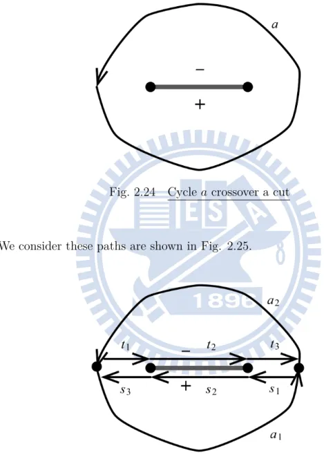
First, consider an a-cycle is shown in Fig. 2.24.

Fig. 2.24 Cycle a crossover a cut

We consider these paths are shown in Fig. 2.25.

Notice that, by the Cauchy’s integral theorem, ∫ t1 f dz + ∫ s3 f dz = 0 ⇒ ∫ t1 f dz =− ∫ s3 f dz, and ∫ t3 f dz + ∫ s1 f dz = 0 ⇒ ∫ t3 f dz =− ∫ s1 f dz.

Again, by the Cauchy integral theorem, { ∫ a1f dz + ∫ s1f dz + ∫ s2f dz + ∫ s3f dz = 0 ∫ a2f dz + ∫ t1f dz + ∫ t2f dz + ∫ t3f dz = 0 ⇒ { ∫ a1f dz + ∫ s1f dz + ∫ s2f dz + ∫ s3f dz = 0 ∫ a2f dz− ∫ s3f dz + ∫ t2f dz− ∫ s1f dz = 0 ⇒ ∫ a1 f dz + ∫ s2 f dz + ∫ a2 f dz + ∫ t2 f dz = 0 ⇒ ∫ a f dz = − ∫ s2 f dz− ∫ t2 f dz ⇒ ∫ a f dz = ∫ r1 f dz + ∫ r2

Next, consider a b-cycle is shown in Fig. 2.27.

Fig. 2.27 Cycle b crossover two cuts

We consider these paths are shown in Fig. 2.28.

Since t1 ∈ − edge of sheet-II = + edge of sheet-I ⇒ ∫ t1 f dz =− ∫ s3 f dz, and t3 ∈ − edge of sheet-II = + edge of sheet-I ⇒ ∫ t3 f dz =− ∫ s1 f dz.

And, by the Cauchy integral theorem, { ∫ b1f dz + ∫ s1f dz + ∫ s2f dz + ∫ s3f dz = 0 ∫ b2f dz + ∫ t1f dz + ∫ t2f dz + ∫ t3f dz = 0 ⇒ { ∫ b1f dz + ∫ s1f dz + ∫ s2f dz + ∫ s3f dz = 0 ∫ b2f dz− ∫ s3f dz + ∫ t2f dz− ∫ s1f dz = 0 ⇒ ∫ b1 f dz + ∫ s2 f dz + ∫ b2 f dz + ∫ t2 f dz = 0 ⇒ ∫ b f dz =− ∫ s2 f dz− ∫ t2 f dz ⇒ ∫ b f dz = ∫ r1 f dz + ∫ r2

Proposition 2.1. If f (z) =

√ n ∑ k=1

(z− zk), where zk are distinct, and the paths r1 and r2

are shown in Fig. 2.30.

Fig. 2.30 Paths r1 and r2 for Pro. 2.1

Prove that ∫ r1 f (z)dz = ∫ r2 f (z)dz. Proof. We know that r1 ∈ + edge of sheet-I =− edge of sheet-II, so ∫ r1 f dz = ∫ r₁′

f dz, where r₁′ is a straight path from zs+1 to zson the − edge of sheet-II. And, since f (z)|(II) = −f(z)|(I),

∫ r₁′ f dz = − ∫ ˜ r1

f dz, where ˜r1 is a straight path

from zs+1 to zs on the − edge of sheet-I. Notice that, ∫ ˜ r1 f dz =− ∫ r2

f (z)dz, and this implies

∫ r1 f (z)dz = ∫ r2 f (z)dz.

Proposition 2.2. If f (z) =

√ n ∑ k=1

(z− zk), where zk are distinct, and the paths r1 and r2

are shown in Fig. 2.31.

Fig. 2.31 Paths r1 and r2 for Pro. 2.2

Prove that ∫ r1 f (z)dz = ∫ r2 f (z)dz. Proof.

We know that f (z)|(II) =−f(z)|(I), so

∫ r2

f (z)dz =−

∫ r2′

f (z)dz, where r′₂ is a straight path from zs+1 to zs in the sheet-I =

∫ r1

Sometimes the integrals over some complicated paths are difficult to compute, so we want to use a computational software program, MATHEMATICA, to obtain the correct value of the integrals over cycles.

Now, we have known the difference between the value in sheet-I and sheet-II of theory, so we just discuss the difference between the value in the sheet-I of theory and in MATHEMATICA, then we can modify the computation in MATHEMATICA such that the numerical result we modified equals the numerical result of theory.

Notice that θ ∈ (−π, π] of reiθ _{in MATHEMATICA, so if ϕ /∈ (−π, π] of re}iϕ_, MATHEMATICA will change reiϕ _{into re}iθ∗_{, such that re}iϕ _{= re}iθ∗ _{and θ}∗ _{∈ (−π, π].}

Lemma 2.1. If z is in the sheet-I for a cut whose one of the end points is zk.

If this cut on the line with the slope m = tan α, 0 < α_{≤ π,} √

z− zk|(I) =

{ √

z− zk|M AT HEM AT ICA if arg(z− zk)∈ (−π, α),

−√z− zk|M AT HEM AT ICA if arg(z− zk)∈ [α − 2π, −π].

Proof.

Let z be in the sheet-I, and using polar form, z_{− z}k = reiθ for some θ ∈ [α − 2π, α). Notice that MATHEMATICA will change reiθ _{into re}iθ∗ _{such that re}iθ _{= re}iθ∗_{, and}

θ∗ ∈ (−π, π].

Case 1: arg(z− zk) = θ∈ (−π, α) Notice that θ ∈ (−π, α) ⊆ (−π, π].

Then θ∗ = θ, and this implies √z− zk|(I) =

√ z− zk|M AT HEM AT ICA. Case 2: arg(z− zk) = θ∈ [α − 2π, −π] Notice that θ _{∈ [α − 2π, −π] " (−π, π], so θ}∗ = θ + 2π∈ [α, π] ⊂ (−π, π]. Then, √ z− zk|(I) = √ reiθ2, and √ z− zk|M AT HEM AT ICA = √ reiθ∗2 =√reiθ+2π2 =−√reiθ2,

and this implies √z− zk|(I) =−

√

Definition 2.1.

Define that

{

f (z)M AT H.= f (z) means f (z)|(I) = f (z)|M AT HEM AT ICA,

f (z)M AT H.= −f(z) means f(z)|(I) =−f(z)|M AT HEM AT ICA.

Next, we will discuss some situations of the domain such that the value in MATH-EMATICA must be modified.

Case 1:

If z is in the sheet-I, and we consider a cut on the line l1(z) = 0 with the slope

m = tan α, 0 < α < π, from z1 to∞, where z1 = x1+ iy1 ∈ C (Fig. 2.32).

Fig. 2.32 Cut with end point z1

1. z ∈ + edge of this cut: arg(z− z1) = α− 2π implies

√ z− z1

M AT H.

= −√z− z1.

2. z ∈ − edge of this cut: arg(z− z1) = α implies

√ z− z1

M AT H.

= √z− z1.

Fig. 2.33 Modified-Value Domain for the cut with end point z1

Case 2:

We consider a cut on the line l1(z) = 0 with the slope m = tan α, 0 < α < π.

Assume without loss of generality that end points of the cut are z1 and z2, ∀zk =

xk+ iyk∈ C (Fig. 2.34).

Fig. 2.34 Cut with end points z1 and z2

Now, we want to find the domain where z belongs, such that

√ z− z1 √ z− z2 M AT H. = −√z− z1 √ z− z2.

1. z _{∈ + edge of this cut:}

(a) arg(z_{− z}1) = α− 2π implies

√ z− z1 M AT H. = −√z− z1. (b) arg(z− z2) = α− π implies √ z− z2 M AT H. = √z− z2. Therefore, √ z− z1 √ z− z2 M AT H. = −√z− z1 √ z− z2.

2. z ∈ − edge of this cut: (a) arg(z− z1) = α implies

√ z− z1 M AT H. = √z− z1. (b) arg(z− z2) = α− π implies √ z− z2 M AT H. = √z− z2. Therefore, √ z− z1 √ z− z2 M AT H. = √z− z1 √ z− z2.

3. z is not on this cut:

By the Lemma 2.1, we know that

√ z− zk

M AT H.

= −√z− zk if arg(z− zk)∈ [α − 2π, −π], and in this sense, consider

         S+ _{={z|z ∈ C, arg(z − z}

1)∈ (−π, α), z is not in the cut},

S− ={z|z ∈ C, arg(z − z1)∈ [α − 2π, −π], z is not in the cut},

T+ _{={z|z ∈ C, arg(z − z}

2)∈ (−π, α), z is not in the cut},

T− ={z|z ∈ C, arg(z − z2)∈ [α − 2π, −π], z is not in the cut}.

⇒            √ z− z1 M AT H. = √z− z1 if z ∈ S+, √ z− z1 M AT H. = −√z− z1 if z ∈ S−, √ z− z2 M AT H. = √z− z2 if z ∈ T+, √ z− z2 M AT H. = −√z− z2 if z ∈ T−.

Fig. 2.35 S+_{, S}−_{, T}+_{, and T}− Then, √z− z1 √ z− z2 M AT H. = −√z− z1 √ z− z2 if and only if z ∈ S+ ∩ T− or z ∈ S−∩ T+. Notice that S+_{∩ T}− _{= ∅, so} √_{z− z} 1 √ z− z2 M AT H. = −√z− z1 √ z− z2 if and only if z _{∈ S}−_{∩ T}+_. Therefore, if z ∈ S−∩ T+ _{={z|z ∈ C, l} 1(z) < 0, y1 ≤ lm(z) < y2}, shown in Fig. 2.36, √ z− z1 √ z− z2 M AT H. = −√z− z1 √ z− z2. Fig. 2.36 S−∩ T+

Case 3:

We consider a horizontal cut from z1 to ∞.

Since the cut is horizontal, its slope m = tan α = 0, and this implies α = π (Fig. 2.37).

Fig. 2.37 Cut with end point z1

1. z ∈ + edge of this cut: arg(z− z1) = −π implies

√ z− z1

M AT H.

= −√z− z1.

2. z ∈ − edge of this cut: arg(z_{− z}1) = π implies

√ z− z1

M AT H.

= √z− z1.

3. z is not in this cut:

Since z is not in this cut, arg(z_{− z}1)∈ (−π, π).

By the Lemma 2.1, we know that

√ z− z1

M AT H.

Case 4:

We consider a horizontal cut with end points are z1 and z2.

Since the cut is horizontal, its slope m = tan α = 0, and this implies α = π (Fig. 2.38).

Fig. 2.38 Cut with end points z1 and z2

1. z ∈ + edge of this cut: (a) arg(z_{− z}1) = 0 implies

√ z− z1 M AT H. = √z− z1. (b) arg(z− z2) =−π implies √ z− z2 M AT H. = −√z− z2. Therefore, √ z− z1 √ z− z2 M AT H. = −√z− z1 √ z− z2.

2. z ∈ − edge of this cut: (a) arg(z− z1) = 0 implies

√ z− z1 M AT H. = √z− z1. (b) arg(z_{− z}2) = π implies √ z− z2 M AT H. = √z− z2. Therefore, √ z− z1 √ z− z2 M AT H. = √z− z1 √ z− z2.

3. z is not on this cut: Suppose that √z− z1 √ z− z2 M AT H. = −√z− z1 √ z− z2.

By the Lemma 2.1, we know that

√ z− zk

M AT H.

= −√z− zk if arg(z− zk) =−π, and in this sense, √z− z1

√ z− z2

M AT H.

= −√z− z1

√

z− z2 if and only if only one

of arg(z− z1) and arg(z− z2) is −π.

Then, z is on the cut, but it is a contradiction.

So, for a horizontal cut with end points are z1 and z2,

√ z− z1 √ z− z2 M AT H. = −√z− z1 √

z− z2 if z ∈ + edge of this cut.

For these different cases, we know that where z belongs for different cuts such that the value in MATHEMATICA must be modified.

Now, the followings are some examples. First, we consider f (z) = √ 7 ∑ k=1 (z− zk), where                          z1 =−1 − i, z2 =−1 + 3i, z3 = 0, z4 = 2, z5 = 3− 2i, z6 = 9 2 + i, and z7 = 6− i.

And, we shown the branch cuts in Fg. 2.39.

Example 2.6. Evaluate ∫_c

1f (z)dz, c1 is shown in Fig. 2.40.

Solution.

We have f (z) = √ 7 ∑ k=1 (z− zk) = 7 ∑ k=1 √

z− zk, and notice that the cycle c1 is simple

connected, so we use the equivalent paths, say c∗₁ = c11∪ c12, shown in Fig. 2.40, such

that c1 ≈ c∗1, where

c11 is the straight path on horizontal cut from z3 to z4 on the + edge of sheet-I, and

c12 is the straight path on horizontal cut from z4 to z3 on the − edge of sheet-I.

1. If z ∈ c11:

By the discussion in this subsection, we have

√ z− z1 √ z− z2 M AT H. = √z− z1 √ z− z2, √ z− z3 √ z− z4 M AT H. = −√z− z3 √ z− z4, √ z− z5 √ z− z6 M AT H. = −√z− z5 √ z− z6, and √ z− z7 M AT H. = −√z− z7, so f (z)M AT H.= −f(z). Thus, ∫ c11 f (z)dz M AT H.= − ∫ 2 0 f (z)dz. 2. If z ∈ c12: By the Proposition 2.1, ∫ c12 f (z)dz = ∫ c11 f (z)dz. Therefore, ∫ c1 f (z)dz = ∫ c∗1 f (z)dz = ∫ c11 f (z)dz + ∫ c12 f (z)dz M AT H. = −2 ∫ 2 0 f (z)dz.

Example 2.7. Evaluate ∫_c

2f (z)dz, c2 is shown in Fig. 2.41.

Solution.

Fig. 2.41 Cycle c2 and the equivalent paths c21, c22, c23, and c24

We consider the equivalent paths, say c∗₂ = c21∪ c22∪ c23∪ c24, shown in Fig. 2.41,

such that c2 ≈ c∗2, where

c21 is the straight path on slant cut from z6 to

7

2− i on the + edge of sheet-I,

c22 is the straight path on slant cut from

7

2 − i to z6 on the − edge of sheet-I,

c23 is the straight path on slant cut from

7

2 − i to z5 on the + edge of sheet-I, and

c24 is the straight path on slant cut from z5 to

7

2− i on the − edge of sheet-I. 1. If z _{∈ c}21:

By the discussion in this subsection, we have √ z− z1 √ z− z2 M AT H. = √z− z1 √ z− z2, √ z− z3 √ z− z4 M AT H. = √z− z3 √ z− z4, √ z− z5 √ z− z6 M AT H. = −√z− z5 √ z− z6, and √ z− z7 M AT H. = −√z− z7, so f (z)M AT H.= f (z). Thus, ∫ c21 f (z)dz M AT H.= ∫ 1 0 f ((9 2+ i) + (−1 − 2i)k)(−1 − 2i)dk. 2. If z ∈ c22: By the Proposition 2.1, ∫ c22 f (z)dz = ∫ c21 f (z)dz. 3. If z ∈ c23: Let z = (7 2 − i) + [z5− ( 7 2− i)]k = (7 2 − i) + (− 1

2− i)k, where k is from 0 to 1, then dz = (−1

2 − i)dk.

By the discussion in this subsection, we have

√ z− z1 √ z− z2 M AT H. = √z− z1 √ z− z2, √ z− z3 √ z− z4 M AT H. = √z− z3 √ z− z4, √ z− z5 √ z− z6 M AT H. = −√z− z5 √ z− z6, and √ z− z7 M AT H. = √z− z7, so f (z)M AT H.= −f(z). Thus, ∫ f (z)dz M AT H.= − ∫ 1 f ((7 − i) + (−1− i)k)(−1 − i)dk.

4. If z _{∈ c}24: By the Proposition 2.1, ∫ c24 f (z)dz = ∫ c23 f (z)dz. Therefore, ∫ c2 f (z)dz = ∫ c∗₂ f (z)dz = ∫ c21 f (z)dz + ∫ c22 f (z)dz + ∫ c23 f (z)dz + ∫ c24 f (z)dz M AT H. = 2 ∫ 1 0 f ((9 2 + i) + (−1 − 2i)k)(−1 − 2i)dk − 2 ∫ 1 0 f ((7 2− i) + (− 1 2 − i)k)(− 1 2− i)dk. Example 2.8. Evaluate ∫_d 1f (z)dz, d1 is shown in Fig. 2.42. Solution.

We consider the equivalent paths, say d∗₁ = d11∪ d12∪ d13∪ d14, shown in Fig. 2.42,

such that d1 ≈ d∗1, where

d11 is the straight path from z5 to

5

2 − i in the sheet-I,

d12 is the straight path from

5

2− i to z5 in the sheet-II,

d13 is the straight path from

5

2− i to z4 in the sheet-I, and

d14 is the straight path from z4 to

5 2 − i in the sheet-II. 1. If z _{∈ d}11: Let z = z5+ [( 5 2 − i) − z5]k = (3− 2i) + (−1

2 + i)k, where k is from 0 to 1, then dz = (−1

2 + i)dk.

By the discussion in this subsection, we have

√ z− z1 √ z− z2 M AT H. = √z− z1 √ z− z2, √ z− z3 √ z− z4 M AT H. = √z− z3 √ z− z4, √ z− z5 √ z− z6 M AT H. = −√z− z5 √ z− z6, and √ z− z7 M AT H. = √z− z7, so f (z)M AT H.= −f(z). Thus, ∫ d11 f (z)dz M AT H.= − ∫ 1 0 f ((3− 2i) + (−1 2 + i)k)(− 1 2 + i)dk. 2. If z _{∈ d}12: By the Proposition 2.2, ∫ d12 f (z)dz = ∫ d11 f (z)dz.

3. If z _{∈ d}13: Let z = (5 2 − i) + [z4− ( 5 2− i)]k = (5 2 − i) + (− 1

2+ i)k, where k is from 0 to 1, then dz = (−1

2 + i)dk.

By the discussion in this subsection, we have

√ z− z1 √ z− z2 M AT H. = √z− z1 √ z− z2, √ z− z3 √ z− z4 M AT H. = √z− z3 √ z− z4, √ z− z5 √ z− z6 M AT H. = −√z− z5 √ z− z6, and √ z− z7 M AT H. = −√z− z7, so f (z)M AT H.= f (z). Thus, ∫ d13 f (z)dz M AT H.= ∫ 1 0 f ((5 2− i) + (− 1 2 + i)k)(− 1 2 + i)dk. 4. If z ∈ d14: By the Proposition 2.2, ∫ d14 f (z)dz = ∫ d13 f (z)dz. Therefore, ∫ d1 f (z)dz = ∫ d∗₁ f (z)dz ∫ ∫ ∫ ∫

Example 2.9. Evaluate ∫_d

2f (z)dz, d2 is shown in Fig. 2.43.

Solution.

Fig. 2.43 Cycle d2 and the equivalent paths d∗1, c12, d21, d22, d23, d24, and d25

We consider the equivalent paths, say d∗₂ = d∗₁ ∪ c12∪ d21∪ d22 ∪ d23∪ d24∪ d25,

shown in Fig. 2.43, such that d2 ≈ d∗2, where

d21 is the straight path on horizontal cut from z3 to z4 on the + edge of sheet-II,

d22 is the straight path from z3 to−

1

3 + i in the sheet-I,

d23 is the straight path from −

1

3 + i to z3 in the sheet-II,

d24 is the straight path from −

1

3 + i to z2 in the sheet-I, and

d25 is the straight path from z2 to−

1

3 + i in the sheet-II.

To start with, we know that d21 is also the straight path on horizontal cut from z3

to z4 on the− edge of sheet-I, that is, d21=−c12, and this implies

∫ c12 f (z)dz + ∫ d21 f (z)dz = 0

1. If z _{∈ d}22: Let z = z3 + [(− 1 3+ i)− z3]k = (−1

3+ i)k, where k is from 0 to 1, then dz = (−1

3 + i)dk.

By the discussion in this subsection, we have

√ z− z1 √ z− z2 M AT H. = √z− z1 √ z− z2, √ z− z3 √ z− z4 M AT H. = √z− z3 √ z− z4, √ z− z5 √ z− z6 M AT H. = −√z− z5 √ z− z6, and √ z− z7 M AT H. = −√z− z7, so f (z)M AT H.= f (z). Thus, ∫ d22 f (z)dz M AT H.= ∫ 1 0 f ((−1 3 + i)k)(− 1 3+ i)dk. 2. If z ∈ d23: By the Proposition 2.2, ∫ d23 f (z)dz = ∫ d22 f (z)dz. 3. If z ∈ d24: Let z = (−1 3+ i) + [z2− (− 1 3 + i)]k

By the discussion in this subsection, we have √ z− z1 √ z− z2 M AT H. = √z− z1 √ z− z2, √ z− z3 √ z− z4 M AT H. = √z− z3 √ z− z4, √ z− z5 √ z− z6 M AT H. = √z− z5 √ z− z6, and √ z− z7 M AT H. = −√z− z7, so f (z)M AT H.= −f(z). Thus, ∫ d24 f (z)dz M AT H.= − ∫ 1 0 f ((−1 3 + i) + (− 2 3+ 2i)k)(− 2 3+ 2i)dk. 4. If z ∈ d25: By the Proposition 2.2, ∫ d25 f (z)dz = ∫ d24 f (z)dz. Therefore, ∫ d2 f (z)dz = ∫ d∗2 f (z)dz = ∫ d∗₁ f (z)dz + ∫ c12 f (z)dz + ∫ d21 f (z)dz + ∫ d22 f (z)dz + ∫ d23 f (z)dz + ∫ d24 f (z)dz + ∫ d25 f (z)dz M AT H. = ∫ d∗1 f (z)dz + 2 ∫ 1 0 f ((−1 3 + i)k)(− 1 3 + i)dk. − 2 ∫ 1 0 f ((−1 3+ i) + (− 2 3+ 2i)k)(− 2 3+ 2i)dk.

The Pendulum Motion on Riemann

Surface

Recall that the sine-Gordon equation is

utt− uxx+ sin[u(x, t)] = 0, where − ∞ < x < ∞ and t > 0. If we let s = αx_{− βt, by the Chain rule:}

         ∂ ∂x = ∂ ∂s ∂s ∂x = α ∂ ∂s, ∂ ∂t = ∂ ∂s ∂s ∂t =−β ∂ ∂s. ⇒          ∂2_u ∂x2 = ∂ ∂x ∂ ∂xu = α 2∂2u ∂s2, ∂2_u ∂t2 = ∂ ∂t ∂ ∂tu = β 2∂2u ∂s2.

Therefore, the Sine-Gorden equation comes to

β2uss− α2uss+ sin[u(s)] = 0. We let β2− α2 _{= 1, the equation is written as}

uss+ sin[u(s)] = 0. (3.1) Notice that we can regard (3.1) as the simple pendulum motion at time s with the

Multiplying an integral factor us to equation (3.1), and we integral it with respect to s: uss+ sin(u) = 0 ⇒ ususs+ ussin(u) = 0 ⇒ ∫ [ususs+ ussin(u)]ds = 0 ⇒ 1 2u 2

s− cos(u) = E, where E is constant,

⇒ us =±

√

2[E + cos(u)].

Since us is the angular velocity, the plus-minus sign means direction, and assume without loss of generality that

us = √

2[E + cos(u)]. (3.2) Next, using the skill in previous chapter, we will solve the problem of pendulum by approximation.

Notice that, by the Taylor series of cos u at 0, cos u ≈ 1 −u 2 2! + u4 4! − u6 6! + u8 8!. Then, the equation (3.2) comes to us=

√ 2[E + 1− u 2 2! + u4 4! − u6 6! + u8 8!].

Now, we consider the situation of E = 0, and by using the MATHEMATICA, we have us= √ 2[1− u 2 2! + u4 4! − u6 6! + u8 8!] = v u u t∏8 k=1 (u− uk), where           u1 =−4.8947 − 2.4869i, u2 =−4.8947 + 2.4869i,

Therefore, we get eight branch points and four branch cuts, shown in Fig. 3.1.

Fig. 3.1 Branch points and the branch cuts of us

For convience, we let f (u) = v u u t∏8 k=1 (u− uk). Notice that, us= du ds = f (u), and ds = 1 f (u)du ⇒ s = ∫ 1 f (u)du.

By the Cauchy integral formula, for any closed path in R of genus 3 is homotopic to an integral combination of the loop-cuts ai and bi, i = 1, 2, 3, so we will consider the integrals of 1

We shown a-cycles in Fg. 3.2.

a1-cycle

We consider the equivalent paths, say a∗₁ = a11∪ a12, shown in Fig. 3.3, such that

a1 ≈ a∗1, where

a11 is the straight path on vertical cut from u2 to u1 on the + edge of sheet-I, and

a12 is the straight path on vertical cut from u1 to u2 on the − edge of sheet-I.

Fig. 3.3 The equivalent paths of a1-cycle

We shown the detail of the integrals in Appendix A.1. Therefore, ∫ a1 1 f (u)du = ∫ a∗1 1 f (u)du = ∫ a11 1 f (u)du + ∫ a12 1 f (u)du M AT H. = 2 ∫ u1 u2 1 f (u)du.

a2-cycle

We consider the equivalent paths, say a∗₂ = a21∪ a22, shown in Fig. 3.4, such that

a2 ≈ a∗2, where

a21 is the straight path on horizontal cut from u3 to u4 on the + edge of sheet-I, and

a22 is the straight path on horizontal cut from u4 to u3 on the − edge of sheet-I.

Fig. 3.4 The equivalent paths of a2-cycle

We shown the detail of the integrals in Appendix A.2. Therefore, ∫ a2 1 f (u)du = ∫ a∗2 1 f (u)du = ∫ a21 1 f (u)du + ∫ a22 1 f (u)du M AT H. = 2 ∫ u4 u3 1 f (u)du.

a3-cycle

We consider the equivalent paths, say a∗₃ = a31∪ a32, shown in Fig. 3.5, such that

a3 ≈ a∗3, where

a31 is the straight path on horizontal cut from u5 to u6 on the + edge of sheet-I, and

a32 is the straight path on horizontal cut from u6 to u5 on the − edge of sheet-I.

Fig. 3.5 The equivalent paths of a3-cycle

We shown the detail of the integrals in Appendix A.3. Therefore, ∫ a3 1 f (u)du = ∫ a∗3 1 f (u)du = ∫ a31 1 f (u)du + ∫ a32 1 f (u)du M AT H. = 2 ∫ u6 u5 1 f (u)du.

We shown b-cycles in Fg. 3.6.

b3-cycle

We consider the equivalent paths, say b∗₃ = b31∪ b32, shown in Fig. 3.7, such that

b3 ≈ b∗3, where

b31 is the straight path from u6 to u8 in the sheet-I, and

b32 is the straight path from u8 to u6 in the sheet-II.

Fig. 3.7 The equivalent paths of b3-cycle

We shown the detail of the integrals in Appendix A.4. Therefore, ∫ b3 1 f (u)du = ∫ b∗3 1 f (u)du = ∫ b31 1 f (u)du + ∫ b32 1 f (u)du M AT H. = −2 ∫ u8 u6 1 f (u)du.

b2-cycle

We consider the equivalent paths, say b∗₂ = b∗₃ ∪ a31∪ b21∪ b22∪ b23, shown in Fig.

3.8, such that b2 ≈ b∗2, where

b21 is the straight path on horizontal cut from u6 to u5 on the − edge of sheet-II,

b22 is the straight path from u4 to u5 in the sheet-I, and

b23 is the straight path from u5 to u4 in the sheet-II.

Fig. 3.8 The equivalent paths of b2-cycle

We shown the detail of the integrals in Appendix A.5. Therefore, ∫ b2 1 f (u)du = ∫ b∗2 1 f (u)du = ∫ b∗₃ 1 f (u)du + ∫ a31 1 f (u)du + ∫ b21 1 f (u)du + ∫ b22 1 f (u)du + ∫ b23 1 f (u)du M AT H. = ∫ 1 du− 2 ∫ u5 ₁ du.

b1-cycle

We consider the equivalent paths, say b∗₁ = b∗₂ ∪ a21∪ b11∪ b12∪ b13, shown in Fig.

3.9, such that b1 ≈ b∗1, where

b11 is the straight path on horizontal cut from u4 to u3 on the − edge of sheet-II,

b12 is the straight path from u1 to u3 in the sheet-I, and

b13 is the straight path from u3 to u1 in the sheet-II.

Fig. 3.9 The equivalent paths of b1-cycle

We shown the detail of the integrals in Appendix A.6. Therefore, ∫ b1 1 f (u)du = ∫ b∗1 1 f (u)du = ∫ b∗₂ 1 f (u)du + ∫ a21 1 f (u)du + ∫ b11 1 f (u)du + ∫ b12 1 f (u)du + ∫ b13 1 f (u)du M AT H. = ∫ b∗₂ 1 f (u)du− 2 ∫ u3 u1 1 f (u)du.

The Elliptic Functions

4.1

Definition and Properties of Elliptic Functions

Definition 4.1. (Doubly-Period Function and Elliptic Function)

We call a function f :_{C → C, a doubly-period function with periods 2ω}1 and 2ω2,

where ω1 and ω2 in C with

ω1

ω2

/

∈ R, if

f (z + 2ω1) = f (z), and f (z + 2ω2) = f (z), for any z∈ C.

And, a doubly-period function which is analytic except at poles, and which has no singularities other than poles in finite part of the plane, is called an elliptic function.

We consider a parallelogram with vertices 0, 2ω1, 2ω2, and 2ω1+ 2ω2. If there is no

point ω inside or on the boundary except vertices of this parallelogram such that

f (z + ω) = f (z), for any z ∈ C,

this parallelogram is called a fundamental period-parallelogram for an elliptic function with period 2ω1 and 2ω2.

In addition, the whole plane may be covered with a network of parallelograms equal to the fundamental period-parallelogram and similarly situated, notice that, all vertices in the form of 2mω1 + 2nω2, ∀m, n ∈ Z, then these parallelograms are called

period-parallelograms. If there is no point ω inside or on the boundary except vertices of

Proposition 4.1.

1. The number of poles of an elliptic function in any cell is finite. 2. The number of zeros of an elliptic function in any cell is finite.

3. The sum of the residues of an elliptic function, f (z), at its poles in any cell is zero. 4. (Liouville’s theorem) An elliptic function, f (z), with no poles in a cell is merely

a constant.

4.2

The Theta-Functions

Let τ be a constant complex number with Im(τ ) is positive, and let q = eπiτ_{, so} that _{|q| < 1.}

To begin with, we let

ϑ0(z, q) = ∞ ∑ n=−∞ (−1)nqn2e2niz = 1 + 2 ∞ ∑ n=1 (−1)nqn2cos(2nz), and we use this function to define the Theta-functions.

Definition 4.2. (The Four Types of the Theta-Functions)

Define that      ϑ1(z, q) = ϑ0(z + 1₂π, q), ϑ2(z, q) = −ieiz+ 1 4πiτϑ₀(z + 1 2πτ, q), and ϑ3(z, q) = ϑ2(z + 1₂π, q). Thus, we have  _∑

Since the parameter q will usually not be specified, ϑi(z) will be written for ϑi(z, q),

i = 0, 1, 2, 3. But if τ is specified, it will be written as ϑ(z|τ). We also denote ϑi(0) = ϑi, and ϑ′_i(0) = ϑ′_i, i = 0, 1, 2, 3.

It is obvious that

ϑ0(z + π) = ϑ0(z), and

ϑ0(z + πτ ) =−q−1e−2izϑ0(z),

and so ϑ0(z) is a quasi doubly-periodic function of z with multipliers 1 and −q−1e−2iz,

associated with the periods π and πτ respectively. In like manner, we get that

ϑ0(z + π) = ϑ0(z), ϑ0(z + πτ ) =−q−1e−2izϑ0(z),

ϑ1(z + π) = ϑ1(z), ϑ1(z + πτ ) = q−1e−2izϑ1(z),

ϑ2(z + π) =−ϑ2(z), ϑ2(z + πτ ) =−q−1e−2izϑ2(z),

ϑ3(z + π) =−ϑ3(z), and ϑ3(z + πτ ) = q−1e−2izϑ3(z).

It is clear that if z0 be any zero of any one of these Theta-functions, so is

z0+ mπ + nπτ,

for all integral values of m and n, and by the Def. 4.2, we know that              ϑ0(z) = 0, if z = πτ 2 +mπ + nπτ, ϑ1(z) = 0, if z = π 2 + πτ 2 +mπ + nπτ, ϑ2(z) = 0, if z = 0 +mπ + nπτ, and ϑ3(z) = 0, if z = π 2 +mπ + nπτ. Proposition 4.2. 1. ϑ2 3(z)ϑ20 = ϑ20(z)ϑ23 − ϑ22(z)ϑ21 2. ϑ2 2(z)ϑ20 = ϑ21(z)ϑ23 − ϑ23(z)ϑ21

Now, we consider ϑ2(z)

ϑ0(z)

and ϑ3(z)ϑ1(z)

ϑ2 0(z)

, it is obvious that they both has multipliers

−1 and 1 associated with the periods π and πτ respectively, so do the derivative of the

former, d dz[ ϑ2(z) ϑ0(z) ] = ϑ ′ 2(z)ϑ0(z) + ϑ2(z)ϑ′0(z) ϑ2 0(z) . Notice that d dz[ ϑ2(z) ϑ0(z) ] ϑ3(z)ϑ1(z) ϑ2 0(z)

is a doubly-periodic function with periods π and 1

2πτ , then by the Liouville’s theorem and as z → 0, it is a constant, that is ϑ

2 0. Therefore, d dz[ ϑ2(z) ϑ0(z) ] = ϑ2₀[ϑ3(z)ϑ1(z) ϑ2 0(z) ], by letting ξ = ϑ2(z) ϑ0(z)

, and using the propo-sition 4.2, it comes to (dξ dz) 2 _{= (ϑ}2 3− ξ 2_ϑ2 1)(ϑ 2 1− ξ 2_ϑ2 3). (4.1) Finally, we write y = ξϑ1 ϑ3 , u = zϑ2 1, and k = ( ϑ3 ϑ1

)2, the equation (4.1) with the particular solution ϑ2(z) ϑ0(z) may be written (dy du) 2 _{= (1− y}2_{)(1− k}2_y2₎

with the particular solution y = ϑ1

ϑ3

ϑ2(uϑ−21 )

ϑ0(uϑ−21 )

4.3 The Jacobian Elliptic Functions

Notice that, in above section, the differential equation (dy

du)

2 _{= (1− y}2_{)(1− k}2_y2₎

has the particular solution

y = ϑ1 ϑ3

ϑ2(uϑ−21 )

ϑ0(uϑ−21 )

.

The differential equation may be written

u = ∫ y 0 1 √ (1− t2₎₍₁− k2_t2₎dt,

and we let y = sn(u, k) or simply y = sn(u). Notice that, √ 1

(1− t2₎₍₁− k2_t2₎ occurs on

Riemann surface of genus 1.

The sine-Gordon Equation

5.1

The Special Solutions of the sine-Gordon

Equa-tion

Recall that the sine-Gordon equation is

utt− uxx+ sin[u(x, t)] = 0, where − ∞ < x < ∞ and t > 0. In chapter 3, we use the method of substitution such that it comes to

uss+ sin[u(s)] = 0, and it implies

1 2u

2

s− cos(u) = E, where E is constant, (5.1)

⇒ us =±

√

2[E + cos(u)]. We focus on us =

√

2[E + cos(u)], and since cos(u) = 1− 2 sin2₍u

2), we have us = √ 2[E + 1− 2 sin2₍u 2)] = √ 2(E + 1)− 4 sin2(u 2). (5.2)

Then we can obtain

s = ∫ u(s) 1 √ − 4 sin2 U dU. (5.3)

By the equation (5.1), we have

1 2u

2

s+ [1− cos(u)] = E + 1,

and regard it as a energy system with the kinetic energy 1 2u

2

s, the potential energy 1− cos(u), and the total energy E +1. Obvious that, all of them are greater than 0, but, since 0≤ [1 − cos(u)] ≤ 2, so we will discuss in four cases by given E in different conditions,

         E + 1 = 0, 0 < E + 1 < 2, E + 1 = 2, and E + 1 > 2. Case 1: E + 1 = 0

When E + 1 = 0, means the total energy is 0, so the pendulum is stationary, and it implies u(s) = 0. Case 2: 0 < E + 1 < 2 By the equation (5.3), s = ∫ u(s) ₁ √ dU

Now, we let t = √ 2 E + 1sin( U 2), so that 1 √ 1− _E+12 sin2₍U 2) = √ 1 1− t2, and dt = 1 2 √ 2 E + 1cos( U 2)dU = 1 2 √ 2 E + 1 √ 1− sin2(U 2)dU = 1 2 √ 2 E + 1 − 2 E + 1sin 2₍U 2)dU = 1 2 √ 2 E + 1 − t 2_dU ⇒ dU = √ 2 2 E+1 − t2 dt. Therefore, s = √ 1 2(E + 1) ∫ u(s) 0 1 √ 1− t2dU = √ 1 2(E + 1) ∫ √ 2 E+1sin( u(s) 2 ) 0 1 √ 1− t2 2 √ 2 E+1 − t 2 dt = ∫ √ 2 E+1sin( u(s) 2 ) 0 1 √ 1− t2 2 √ 4− 2(E + 1)t2dt = ∫ √ 2 E+1sin( u(s) 2 ) 0 1 √ 1− t2 1 √ 1− E+1₂ t2 dt. And, let k = √ E + 1 2 , then s = ∫ 1 ksin( u(s) 2 ) 0 1 √ 1− t2 1 √ 1− k2_t2dt. (5.4)

Finally, by the Jacobian elliptic function, sn(s, k) = 1

k sin( u(s)

2 ) with 0 < k < 1, and this implies that

Case 3: E + 1 = 2 By the equation (5.3), s = 1 2 ∫ u(s) 0 1 √ 1− sin2(U₂) dU. Let t = sin(U 2), so that 1 √ 1− sin2(U₂) = √ 1 1− t2, and dt = 1 2cos( U 2)dU = 1 2 √ 1− sin2(U 2)dU = 1 2 √ 1− t2_dU ⇒ dU = √ 2 1− t2dt. Therefore, s = 1 2 ∫ u(s) 0 1 √ 1− t2dU = 1 2 ∫ sin(u(s)₂ ) 0 1 √ 1− t2 2 √ 1− t2dt = ∫ sin(u(s)₂ ) 0 1 √ 1− t2 1 √ 1− t2dt. (5.5)

Finally, by the Jacobian elliptic function for k = 1, sn(s, 1) = sin(u(s)

2 ), and this implies that

Case 4: E + 1 > 2 By the equation (5.3), s = √ 1 2(E + 1) ∫ u(s) 0 1 √ 1− _E+12 sin2(U₂) dU. Let k = √ 2 E + 1 and t = sin( U 2), so that 1 √ 1− _E+12 sin2₍U 2) = √ 1 1− k2_t2, and dt = 1 2cos( U 2)dU = 1 2 √ 1− sin2₍U 2)dU = 1 2 √ 1− t2_dU ⇒ dU = √ 2 1− t2dt. Therefore, s = √ 1 2(E + 1) ∫ u(s) 0 1 √ 1− k2_t2dU = k 2 ∫ sin(u(s)₂ ) 0 1 √ 1− k2_t2 2 √ 1− t2dt = k ∫ sin(u(s)₂ ) 0 1 √ 1− t2 1 √ 1− k2_t2dt ⇒ s k = ∫ sin(u(s)₂ ) 0 1 √ 1− t2 1 √ 1− k2_t2dt.

Finally, by the Jacobian elliptic function, sn(s

k, k) = sin( u(s)

2 ) with 0 < k < 1, and this implies that

u(s) = 2 arcsin[sn(s k, k)].

5.2 The Periods of Those Solutions

To begin with, suppose that the pendulum released with no initial velocity, and has the period T .

Notice that, when this pendulum first passes through to bottom equilibrium posi-tion, it spent the time T

4, and so the initial angle is u(

T

4).

Case 1: E + 1 = 0

Since the pendulum is stationary, T = 0.

Case 2: 0 < E + 1 < 2

Notice that, in the discussion of above section, k = √

E + 1

2 . We consider the initial position, the energy system is

1− cos[u(T 4)] = E + 1 ⇒ 2 sin2[u( T 4) 2 ] = 2k 2 ⇒ u(T 4) = ±2 arcsin k. Assume without loss of generality that u(T

4) = 2 arcsin k. By the equation (5.4), T = 4(T 4) = 4 ∫ 1 ksin( u( T₄) 2 ) 0 1 √ 1− t2 1 √ 1− k2_t2dt = 4 ∫ 1 ksin(arcsin k) 0 1 √ 1− t2 1 √ 1− k2_t2dt = 4 ∫ 1 ₁ √ √ 1 dt.

Case 3: E + 1 = 2

We consider the initial position, the energy system is 1− cos[u(T 4)] = E + 1 = 2 ⇒ cos[u(T 4)] = −1 ⇒ u(T 4) = ±π. Assume without loss of generality that u(T

4) = π. By the equation (5.5), T = 4(T 4) = 4 ∫ sin(u( T4) 2 ) 0 1 √ 1− t2 1 √ 1− t2dt = 4 ∫ sin(π 2) 0 1 1− t2dt = 4 ∫ 1 0 1 1− t2dt =∞. So, the period is ∞.

Case 4: E + 1 > 2

Now, we want to find out the exact period, but the equation (5.2) always positive for E +1 > 2, and this means that the pendulum doesn’t change the direction, and always have velocity for every position. Thus, the pendulum will never stop, and never swing back, so this implies it have no periodicity.