海洋大陸森林砍伐及其伴隨火災與氣候之關係

(1)

國立臺灣大學理學院大氣科學系碩士論文

Department of Atmospheric Sciences College of Science

National Taiwan University Master Thesis

海洋大陸森林砍伐及其伴隨火災與氣候之關係 The Relation between Climate and Deforestation in the

Maritime Continent

陳竹君 Chu-Chun Chen

指導教授：羅敏輝博士 Advisor: Min-Hui Lo, Ph.D.

中華民國 106 年 1 月

January 2017

(2)

口試委員會審定書

(3)

謝辭

這本論文的完成，首先要感謝我的指導教授羅敏輝老師，從大三的獨立研究至今，四年多的耐心指導，老師對科學研究的熱情一直是我們的典範，每次研究上遇到挫折，和老師聊聊總是能讓我重拾希望，謝謝老師在我幾乎要放棄的時刻還是願意支持我，給了我很多力量繼續走下去。

感謝許晃雄老師、陳維婷老師、吳健銘老師、黃彥婷老師撥冗擔任口試委員，

並給予許多寶貴的建議及想法，使本論文更臻完善。特別要感謝陳維婷老師、吳健銘老師在每次聯合研究室討論時給予的建議與鼓勵，使我能在研究的道路上有

更寬闊的視野。此外，還要感謝在 UCI 時余進義老師的指導，尤其論文第二部分，

要感謝余老師時常與我們討論並給予許多建議與幫助。

在大學及研究所的生活中，要感謝大氣系的所有人給予我成長的養分，栽培我成為現在的我。謝謝小毛在我成為研究生的路上給予的協助與支持。謝謝禹喬學長在研究上時常與我討論、給我很多想法與方向。謝謝排球校隊、系隊的大家，

讓我在研究之餘還有一個可以揮灑青春的地方。謝謝陸地水文氣候及衛星遙測實驗室的每位夥伴，謝謝你們在我有任何問題時總是熱心地給予我協助，是我最堅

強的靠山。謝謝C404，這裡就像我的第二個家，不只是因為我常常在這裡值夜班，

還有每個人給的溫暖與陪伴，讓深夜的實驗室不孤單。

最重要的是，謝謝我的家人，謝謝你們無條件的支持，讓我能夠有勇氣做我自己。最後，謹將此論文獻給所有幫助過我的人。

(4)

摘要

熱帶雨林地區之森林砍伐會造成地表能量收支及水循環的改變，進一步影響局地甚至全球之氣候。本研究利用地球系統模式模擬海洋大陸地區森林砍伐對氣候造成的影響。模擬結果顯示森林砍伐會導致該地區地表溫度上升及降水增加。

藉由分析垂直積分水氣收支以及濕靜能收支，可以發現地表增溫效應以及低層水氣輻合帶來中層水氣增加的效應共同造成了森林砍伐地區的大氣不穩定，增強上升運動，伴隨更多的水氣輻合，抵銷了森林砍伐後的蒸發散量減少，因而使該地區降水增加。此外，森林砍伐導致海洋大陸地區的上升運動增強，伴隨中太平洋的下沉運動，此環流變化可能會影響沃克環流，進一步影響其他地區的氣候。

海洋大陸地區的森林砍伐除了地表植被的變化之外，通常會伴隨森林火災，

而此地區的森林火災強度會受到氣候影響，尤其以聖嬰事件的影響最為顯著。聖嬰事件可以分為東太平洋以及中太平洋聖嬰事件，其中東太平洋聖嬰事件由於海溫異常中心偏東，相較中太平洋聖嬰事件，其造成的沃克環流改變會在婆羅洲南部有更強的下沉運動異常，導致該地區乾季延長至十月，森林火災持續蔓延，造成東太平洋聖嬰事件時婆羅洲南部有較多的火點數量。過去預測此地區的森林火災通常考慮的是聖嬰事件的強度，本研究顯示考慮聖嬰事件的類型可能比考慮其強度重要，此發現將有助於婆羅洲南部森林火災之預報。

關鍵字：海洋大陸、熱帶雨林、森林砍伐、森林火災、聖嬰事件

(5)

Abstract

Deforestation in tropical regions would lead to changes in local energy and moisture budget, resulting in further impacts on regional and global climate. Previous studies have indicated that the reduction of evapotranspiration dominates the influence of tropical deforestation, which causes a warmer and drier climate locally. Most studies agree that the deforestation leads to an increase in temperature and decline in precipitation over the deforested area. However, unlike Amazon or Africa, Maritime Continent consists of islands surrounded by oceans so the drying effects found in Amazon or Africa may not be the case in Maritime Continent. Thus, our objective is to investigate the local and remote climate responses to deforestation in such unique region. We conduct deforestation experiments using NCAR Community Earth System Model (CESM) and through converting the tropical rainforest into grassland. The results show that deforestation in Maritime Continent leads to an increase in both temperature and precipitation. Moisture budget analysis indicates that the increase in precipitation is associated with the vertically integrated vertical moisture advection, especially the dynamic component (changes in convection). In addition, through moist static energy (MSE) budget analysis, we find the atmosphere among deforested areas become unstable owing to the combined effects of higher specific humidity and temperature in the mid-level. This instability will induce anomalous ascending motion, which could

(6)

enhance the low-level moisture convergence, providing water vapor from the surrounding warm ocean. Besides the increased precipitation, the enhanced ascending motion over Maritime Continent may participate in the changes in Pacific Walker circulation, producing possible remote climate impacts beyond the tropics.

The deforestation in Maritime Continent not only changes the vegetation types and the local climate, but also accompanies the slash-and-burn agricultural fire. Fire activity in Indonesia is strongly linked with El Niño events, whose sea surface temperature (SST) patterns can weaken the Walker circulation leading to a drought condition in the region.

Here we show via case analyses and idealized climate model simulations that it is the central location of the SST anomalies associated with El Niño, rather than its intensity, that is mostly linked with the fire occurrence. During our study period of 1997-2015, Eastern Pacific (EP) El Niño events produced the largest fire events in southern Borneo (i.e., in 1997, 2006, and 2015), while Central Pacific (CP) El Niño events consistently produced minor fire events. The EP El Niño is found to be more capable than the CP El Niño of weakening the Walker circulation that acts to prolong Borneo’s drought condition from September to October. The extended dry conditions in October potentially increase the occurrence of fires during EP El Niño years. The 2015 fire event owes its occurrence to the location of the 2015 El Niño but not necessarily its “Godzilla”

intensity in affecting the fire episodes over southern Borneo. Projecting the location of

(7)

El Niño events might be more important than projecting their strength for fire management in southern Borneo.

Keywords: Maritime Continent, tropical rainforest, deforestation, fire, El Niño

(8)

Figure captions

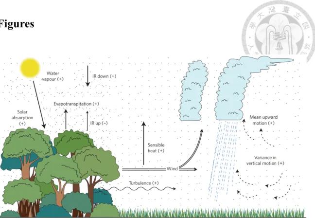
Figure 1.1 Schematic diagram of the enhanced convection over the deforested area

nearby the forest (Anthes, 1984; Lawrence and Vandecar, 2015). ... 39 Figure 1.2 Annual net change in forest area during the 1990-2015 period. From the

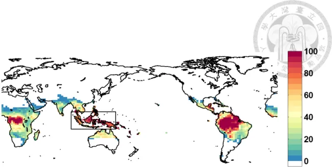
United Nations Food and Agriculture Organization (FAO). ... 40 Figure 1.3 Terra MODIS enhanced vegetation index (EVI) trend during the period

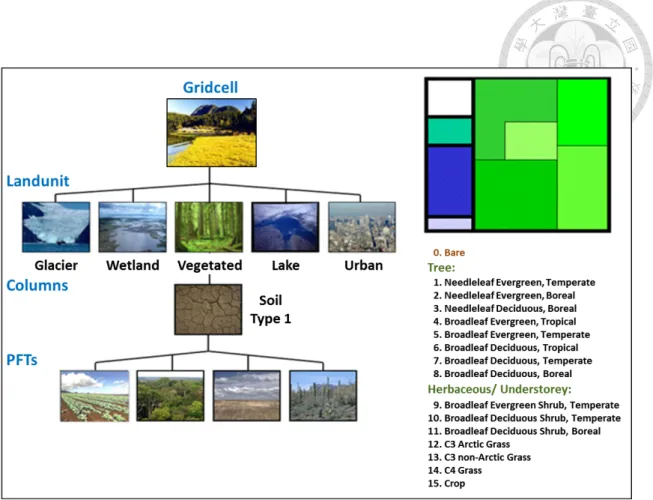
2001-2013. The shaded areas indicate significance at the 95% confidence level. . 41 Figure 2.1 Schematic diagram of the representation of land surface cover types in the Community Land Model version 4 (CLM4.0). From CLM website (http://www.cesm.ucar.edu/models/clm/surface.heterogeneity.html). ... 42 Figure 2.2 Percentage of the vegetation types of rainforest (broadleaf evergreen tropical tree and broadleaf deciduous tropical tree). The black box indicates Maritime Continent. ... 43 Figure 2.3 (a) Annual mean precipitation in CESM control run. (b) TRMM

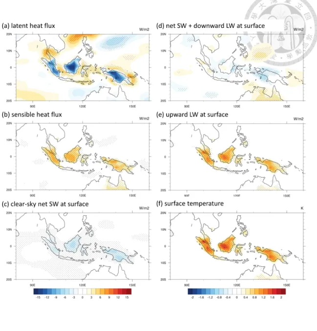
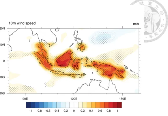
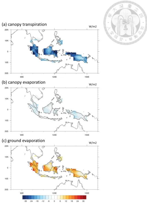
(TMPA3B43) precipitation climatology (averaged from 1998 to 2015). ... 44 Figure 3.1 Difference between the deforestation experimental run and the control run in annual mean (a) surface latent heat flux, (b) surface sensible heat flux, (c) clear-sky net shortwave flux at surface, (d) net shortwave flux and downward longwave flux at surface, (e) upward longwave flux at surface, and (f) surface temperature. Dotted areas indicate p < 0.05. ... 45 Figure 3.2 Same as Figure 3.1 but for annual mean wind speed at 10m above the surface. ... 46 Figure 3.3 Same as Figure 3.1 but for annual mean (a) canopy transpiration, (b) canopy

(10)

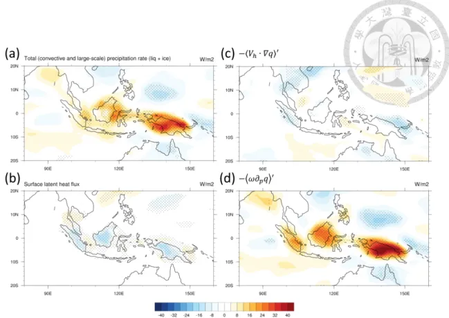
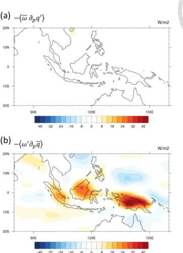
evaporation, (c) ground evaporation. ... 47 Figure 3.4 Same as Figure 3.1 but for annual mean (a) precipitation, (b) surface latent heat flux, (c) vertically integrated horizontal moisture advection, and (d) vertically integrated vertical moisture advection. ... 48 Figure 3.5 Same as Figure 3.1 but for annual mean (a) thermodynamic component and

(b) dynamic component of vertically integrated vertical moisture advection. ... 49 Figure 3.6 Difference between the deforestation experimental run (DEF) and the control run (CTR) in annual mean (a) vertical velocity profile over land and ocean and (b) specific humidity profile over land and ocean. ... 50 Figure 3.7 Same as Figure 3.1 but for annual mean convective precipitation from

Zhang-McFarlane (ZM) deterministic deep convective scheme. ... 51 Figure 3.8 Same as Figure 3.6 but for annual mean MSE profile over land. ... 52

Figure 3.9 Same as Figure 3.1 but for annual mean low level moisture convergence

(integrated from surface to 900 hPa). ... 53 Figure 3.10 Schematic diagram of how deforestation influences precipitation. ... 54

Figure 3.11 Longitude-pressure cross section of the vertical velocity difference between the deforestation experimental run and the control run (averaged between 10°S to 10°N). The shaded areas indicate p < 0.1. ... 55 Figure 4.1 (a) Satellite image of the Maritime Continent and Borneo with area studied delineated by the yellow box (Map created using a Google Maps: Imagery ©2016 TerraMetrics; Map data ©2016 Google). (b) The climatological precipitation in southern Borneo averaged from 1998 to 2010. The shaded area represents the region within one standard deviation of the climatology. (c) Interannual evolution of the southern Borneo fire pixel count and precipitation in October. Types of El

(11)

Niño events and intensities (based on Niño3.4 in October) are indicated at the bottom of the figure. (d) Relationship between southern Borneo fire pixel count and precipitation in October. The blue curve shows an exponential relationship with r²=0.93, p<0.001. ... 56 Figure 4.2 Seasonality of precipitation over southern Borneo during five El Niño events (1997, 2002, 2004, 2006, 2009). The climatology shown by the black dashed line is calculated using data for the period 1998 to 2010. The shaded area represents the region within one standard deviation of the climatology. Data sources include (a) PREC/L and (b) TRMM (TMPA3B43) (excluding the 1997 El Niño event and with 2015 data). ... 57 Figure 4.3 Seasonality of fire pixel count over southern Borneo during five El Niño events (1997, 2002, 2004, 2006, 2009). The climatology shown by the black dashed line is calculated using data for the period 1998 to 2010. The shaded area represents the region within one standard deviation of the climatology. Data sources include (a) ATSR and (b) MODIS (excluding the 1997 El Niño event and with 2015 data). ... 58 Figure 4.4 (a) Seasonality of the fire pixel count over southern Borneo. The climatology shown by the black dashed line is calculated using data for the period 1998 to 2010.

All El Niño composites are shown by the green line, while the red line is for the CP El Niño composite (2002, 2004, and 2009), and the blue line is for EP El Niño composite (1997 and 2006). The shaded area represents the region within 95%

(dark gray) and 99% (light gray) confidence intervals for monthly mean. (b) Same as (a), but for monthly precipitation. ... 59 Figure 4.5 (a) Longitude-time evolution of 250 hPa velocity potential difference

(12)

between 5°N and 5°S from July to October. (b) Same as (a), but for sea surface temperature. (c) Longitude-time evolution of the 250 hPa velocity potential difference between 2015 and CP El Niño composite averaged between 5°N and 5°S from July to October. (d) Same as (c), but for sea surface temperature. ... 60 Figure 4.6 Difference between the EP El Niño composite (i.e., 1997, 2006, and 2015) and the CP El Niño composite (i.e., 2002, 2004, and 2009) in (a) 250 hPa velocity potential and (b) 500 hPa omega from NCEP/NCAR reanalysis, and (c) GPCP precipitation averaged from July to October. ... 61 Figure 4.7 (a) Longitude-time evolution of sea surface temperature difference between the EP El Niño simulations composite and the CP El Niño simulations composite averaged between 5°N and 5°S from July to October. (b) Same as (a), but for the 200 hPa velocity potential. Dotted areas indicate p < 0.05. ... 62 Figure 5.1 (a) Longitude-pressure cross section of ERA Interim vertical velocity trend during the period 2002-2013 (averaged between 10°S to 10°N). (b) ERA Interim zonal wind stress trend during the period 2002-2013. The shaded areas indicate p <

0.05... 63

(13)

Table captions

Table 1.1 Comparison of general circulation model (GCM) experiments of Maritime Continent deforestation. ... 64

(14)

Chapter 1 Introduction

1.1 Tropical rainforest and deforestation

Tropical rainforest plays an important role in both water cycle and land surface energy budget since it is the interface between land and atmosphere. Rainforest trees could act as a water pump, extracting water from the soil into the atmosphere through canopy transpiration (Aragão, 2012). The forest leaves could intercept part of precipitation, and then this interception will evaporate back to the atmosphere without reaching the ground, which is called canopy evaporation. The other part of evaporation that comes from throughfall, canopy drip, and precipitation directly reaching the soil is called ground evaporation. These three processes viewed together are called evapotranspiration (ET) and the latent heat fluxes, which are crucial for the water cycle and energy cycle in the rainforest regions.

Part of this evapotranspiration will become the precipitation falling within the same region, which is called recycled precipitation (Eltahir and Bras, 1996; van der Ent et al., 2010). The rest of precipitation originates from the moisture transported from

other regions through atmospheric transport. The ratio of recycled precipitation to total precipitation is called precipitation recycling ratio. Previous studies have estimated the recycled precipitation could account for 25~56% in the Amazon basin (Molion, 1975;

(15)

Brubaker et al., 1993; Eltahir and Bras, 1994). However, since the recycling ratio depends on the spatial scale and shape of the selected region, it is difficult to compare and integrate these previous estimations. Also, the aforementioned processes and the precipitation recycling ratio may change under recent deforestation in the tropics.

Anthropogenic land use and land cover change, including the deforestation, could have substantial effects on the local and remote climate. For instance, deforestation could directly alter the partitioning of local surface energy and hydrology budget, and might indirectly change the recycling ratio, and thus, the precipitation. The uncertainty of these climate impacts still exists owing to the complex land-atmosphere interactions.

Therefore, the aim of this study is to decipher the local and remote effects of deforestation on climate and have a better understanding of the ongoing climate change.

1.2 Local and remote responses to deforestation

Rainforest trees have larger leaf and stem area for evapotranspiration, lower albedo, and taller tree height compared with other vegetation types. As a result, converting rainforest into the bare ground or grassland will lead to three major impacts: the reduction of evapotranspiration, the increase in surface albedo, and the decrease in surface roughness. The reduction of evapotranspiration will consequently decrease the latent heat flux, thus induce a warming effect on the surface. Besides, the decrease in

(16)

roughness reduces the aerodynamic exchange between the surface and the above atmosphere. Even though the enhanced wind speed might mitigate this effect, the net effect will cause the decrease in evapotranspiration (Maloney, 1998). These two nonradiative processes contribute to the changes in both water and energy budgets, causing a positive temperature response. On the contrary, the radiative process, the increase in surface albedo, will reduce the net incoming radiation and therefore cause a cooling effect. Previous studies have indicated that the nonradiative processes are stronger in the tropics and thus the net response to tropical deforestation is warming, whereas the radiative process plays a more important role in temperate and boreal zones, deforestation in these regions causing a net effect of cooling (Davin and de Noblet-Ducoudré, 2010; Malyshev et al., 2015).

The indirect effects caused by deforestation, such as changes in precipitation, are more complex and have more uncertainty than the direct effects. For example, as mentioned in the previous section, the precipitation recycling ratio is usually high in tropical rainforest regions. However, we cannot claim that the reduction of evapotranspiration results in the decrease in precipitation unless both the precipitation recycling ratio and the atmospheric moisture transport remain the same before and after the deforestation. In fact, the reduction of evapotranspiration may influence both the atmospheric water vapor transport and the precipitation recycling ratio owing to the

(17)

circulation change. This might be one of the reasons that the variation still exist among the studies about the precipitation responses to the tropical deforestation (e.g., Sud et al., 1996; Negri et al., 2004; Ramos da Sliva et al., 2008; Medvigy et al., 2011).

Previous studies about the tropical deforestation consider different spatial scale and various locations surrounded with the different environment and mean climate (e.g., Polcher and Laval, 1994a; Schneck and Mosbrugger, 2011; Lawrence and Vandecar, 2015; Spracklen and Garcia-Carreras, 2015). Large-scale deforestation (thousands km scale) uses the numerical climate model to simulate the idealized deforestation scenario, such as the deforestation throughout the whole tropical rainforest or the complete deforestation within Amazon basin or Congo basin. Basically, these simulations offer a general agreement about the local climate impacts that the large-scale tropical deforestation possibly results in a warmer and drier climate over the deforested region, especially in the Amazon Basin (e.g., Sud et al., 1996; Voldoire and Royer, 2004;

Avissar and Werth, 2005; Ramos da Silva et al. 2008; Lawrence and Vandecar, 2015;

Lejeune et al., 2015; Spracklen and Garcia-Carreras, 2015). The local temperature increases because the larger reduction of surface latent heat flux compensates the smaller decrease in surface net radiation. Meanwhile, the reduction of transpiration contributes to the decrease in precipitation. On the other hand, there are a few studies showing the different temperature and precipitation responses in the Congo basin and

(18)

Maritime Continent (Polcher and Laval, 1994a; McGuffie et al., 1995; Zhang et al., 1996a; Findell et al., 2006). These exceptions may result from the different vegetation types used for deforestation simulations or the deforestation regions are not confined within the tropical belt. Besides the local climate effects, the results suggest large-scale deforestation may induce remote effects through large-scale circulation changes (e.g., Hadley circulation and/or Walker circulation) and Rossby wave propagation (e.g., Henderson-Sellers et al. 1993; Sud et al., 1996; Zhang et al., 1996b; Snyder, 2010, Lawrence and Vandecar, 2015).

Mesoscale deforestation (from tens to hundreds, up to two thousand km scale) surrounded by forest or ocean reflects a more realistic deforestation scenario (e.g., Wang et al., 2000; Roy, 2009; Hanif et al., 2016). Both observation datasets and model

simulations have been used to investigate the impacts of mesoscale deforestation.

Previous studies based on satellite observation and mesoscale model have indicated the heterogeneous land surface, for example, a “fish-bone” deforestation pattern, could induce mesoscale circulation under weak synoptic-scale forcing and further enhance the occurrence of cloudiness and rainfall in western Brazil (Wang et al., 2000; Negri et al., 2004; Roy, 2009) (Figure 1.1). In addition, the regional model simulation shows an increase in precipitation at the edge of the forest in Amazon basin (Ramos da Sliva et al., 2008). Observation datasets also reveal the deforestation tends to increase local

(19)

precipitation in both western Brazil and western Malaysia (Butt et al., 2011; Hanif et al., 2016). However, when it comes to the Maritime Continent, the islands surrounded by ocean, some discrepancies emerge. As shown in Table 1.1, most studies indicate that the deforestation will result in the reduction of precipitation in the Maritime Continent because of the considerable influence of the decrease in latent heat flux (Mabuchi et al., 2005a; Mabuchi et al., 2005b; Werth and Avissar, 2005; Mabuchi, 2011; Kumagai et al., 2013). On the other hand, Schneck and Mosbrugger (2011) show there is enhanced convection over the surrounding ocean using a fully coupled model, and Delire et al.

(2001) find the increased precipitation over the island by using the model with fixed sea surface temperature.

1.3 Deforestation in Maritime Continent

Maritime Continent is one of the three major tropical rainforests. Unfortunately, according to the annual net change in forest area during 1990-2015 (Figure 1.2, from the United Nations Food and Agriculture Organization), Indonesia and Brazil have the largest area of forest loss. Moreover, from Landsat satellite data, the forest clear rate in Indonesia is higher than Brazilian Amazon in recent decade (Margono et al., 2014;

Hasen et al., 2013). We further used enhanced vegetation index (EVI) derived from MODIS satellite data to verify the deforestation in the Maritime Continent. As expected,

(20)

the EVI trend in the recent decade shows the decline over the Maritime Continent (the region in brown color in Figure 1.3). However, there are fewer studies about the influences of deforestation in Maritime Continent compared with those in the Brazilian Amazon. Since the Maritime Continent is located in the ascending region of the Hadley cell and Walker circulation, the climate response to deforestation may further influence other regions through the changes in large-scale circulation. Hence, in this study, we aim to understand the climate response to the deforestation in the Maritime Continent.

Besides the unique climatic role, there is another special characteristic that the deforestation in Maritime Continent often accompanies with forest fire as a method of slash-and-burn agriculture. In the following section, we would further illustrate the relationship between fire and deforestation in Maritime Continent.

1.4 Fire and two types of El Niño

Fire in Indonesia is known to be strongly linked with El Niño events (Field and Shen, 2008; van der Werf et al., 2008; Field et al., 2009; Reid et al., 2012), and has critical impacts on the global carbon budget, tropical biodiversity, ecosystem health, global energy supplies, as well as air quality and human health (Sodhi et al., 2004;

Danielsen et al., 2009; van der Werf et al., 2010; Marlier, 2012). The year of 2015, the fire situation in this region is exceptionally severe (Voiland, 2015). In fact, 2015 was the

(21)

largest fire year since 1997 (van der Werf, 2015) and surpassed the second largest year (2006). Often, fires are set for agricultural purposes, legally or illegally, during the dry season (June to September) in Indonesia (Hendon, 2003). In remote areas, there are few means to contain the burning except waiting for the onset of the wet season (Page et al., 2002). During drought years, fire can evade this control and burn a substantial acreage beyond what was intended of, as in the 2015 fire episode in Indonesian Sumatra and southern Borneo.

Drought events in Indonesia are strongly associated with El Niño events that occur roughly every 2 to 7 years. Coupling of large fire events and El Niño events is well known and greatly acknowledged (van der Werf et al., 2008, 2010). Studies across various tropical and subtropical regions have proved that fire forecast relies at least partially on seasonal El Niño forecasts (Chen et al., 2011; Wooster et al., 2012). El Niño characteristics vary from event to event and successive El Niño events are not identical (Capotondi and Sardeshmukh, 2015). The interannual variability of fire activity is related to the details of the SST patterns associated with the El Niño events (Reid et al., 2012). From the prospect of pre-warning and effective fire management in the region that has a global impact, it is crucial to be able to identify the key features of the El Niño SST patterns that matter to the magnitude of fire activity and to understand the physical linkages between them.

(22)

Chapter 2 Methodology

2.1 Budget analyses and model setup for Chapter 3 2.1.1 Model setup for deforestation experiment

In this study, we used Community Earth System Model (CESM) to examine the climatic effects of deforestation in Maritime Continent. We used “F_2000_CAM5”

component set in CESM, which features year 2000 greenhouse gas concentrations and runs in stand-alone Community Atmosphere Model (CAM) mode with CAM5 physics (Neale et al., 2012). The model runs with a horizontal resolution of 1.9°×2.5° and prescribed climatological sea surface temperatures and sea ice. All the simulations were run for 30 years while the last 25 years were used for analysis. In the Community Land Model Version 4 (CLM4.0) (Oleson et al., 2010; Lawrence et al., 2011), the vegetation types are represented by Plant Functional Type (PFT) (Figure 2.1). Each PFT has its own properties, such as leaf area index, stem area index, and canopy height, thus the albedo or evapotranspiration will change between different PFT. In our deforestation experimental run, the vegetation types of broadleaf evergreen tropical tree and broadleaf deciduous tropical tree were replaced by warm C4 grass, which will most likely grow back in the tropical region (Sage et al., 1999), to represent the deforestation (Figure 2.2).

The precipitation in control run roughly agrees with observations, although the values

(23)

are slightly higher over the South China Sea and are underestimated on the west of Sumatra and within Borneo and Sumatra (Figure 2.3).

2.1.2 Vertically integrated moisture budget

To diagnose the changes in precipitation, we used the vertically integrated moisture budget equation:

𝜕𝑞

𝜕𝑡 = 𝐸𝑇 − 𝑃 − ∇ ⋅ 𝑣𝑞 , (1)

where the 𝑞 is the specific humidity, 𝐸𝑇 is evapotranspiration, 𝑃 is precipitation, 𝑣 is horizontal velocity vector. Angle brackets denote mass integration through the troposphere:

𝑋 =1

𝑔 ³⁴𝑋𝑑𝑝 ,

35

(2) where 𝑔 is the acceleration of gravity, 𝑝₆ is the pressure at the tropopause (100 hPa in this study), and 𝑝₇ is surface pressure. Since the vertical velocity ω is near zero at the surface and tropopause (Tan et al., 2008), the divergence of moisture flux can be estimated as

∇ ⋅ 𝑣𝑞 ≈ 𝑣 ⋅ ∇𝑞 + 𝜔𝜕𝑞

𝜕𝑝 , (3)

where 𝑣 ⋅ ∇𝑞 is the vertically integrated horizontal moisture advection and 𝜔^<=_<3 is the vertically integrated vertical moisture advection. The long-term averaged ^<=_<6 is negligible, so the anomalies for vertically integrated moisture budget equation can be

(24)

written as (Chou and Neelin, 2004; Chou et al., 2006) 𝑃^> ≈ 𝐸𝑇^>− 𝑣 ⋅ ∇𝑞 ^>− 𝜔𝜕𝑞

𝜕𝑝

>

, (4)

where apostrophe ′ represents the differences between control run and deforestation experimental run. The changes in vertically integrated vertical moisture advection can be further divided into two components:

− 𝜔𝜕𝑞′

𝜕𝑝

>

≈ − 𝜔𝜕𝑞^>

𝜕𝑝 − 𝜔′𝜕𝑞′

𝜕𝑝 , (5)

where ( ) is the value from control run and ( )′ is the difference between control run and deforestation experimental run. The first term − 𝜔^<=_<3^B is thermodynamic component, which is associated with changes in water vapor. The second term

− 𝜔′^<=>_<3 is dynamic component, which is associated with changes in convection.

2.1.3 Moist static energy

To understand mechanisms that induce changes in convection, we analyzed the vertical profile of moist static energy (MSE) anomalies. MSE is defined as

MSE = 𝐶_G𝑇 + 𝐿𝑞 + 𝑔𝑧 , (6)

where 𝐶₃ is the specific heat of air at constant pressure and 𝑇 is the temperature, 𝐿 is the latent heat of vaporization, 𝑞 is the specific humidity, 𝑔 is the acceleration of gravity, and 𝑧 is height.

(25)

2.2 Observation datasets and model setup for Chapter 4 2.2.1 Precipitation

Our rainfall data are from National Oceanic and Atmospheric Administration (NOAA)’s Precipitation Reconstruction over Land (PREC/L) (Chen et al., 2002). The product reports monthly average rainfall over land reconstructed from global gauge station observations. In a parallel analysis, we used a TRMM dataset (TMPA 3B43) (Liu et al., 2012) for comparison.

2.2.2 Fire activity in Borneo

The European Space Agency’s (ESA) Advanced Along Track Scanning Radiometer ([A]ATSR) on board various ESA satellites reported (globally) nighttime surface thermal anomalies in the 3.8 micrometer mid-infrared channel from 1995 to 2012 (Arino et al., 2012). We used the ATSR World Fire Atlas (WFA) Algorithm 1 as our primary analysis dataset. We rebinned monthly latitude-longitude records from ATSR to a 0.5°×0.5° resolution raster file for comparison with the precipitation data. Fire generally shows a strong diurnal cycle (Giglio, 2007). Therefore, we performed a parallel analysis using MODIS Terra products (MOD14CMH) (Giglio et al., 2006) with an overpass time in the late morning. The result from MODIS Terra is similar to that from ATSR products, except for a difference in scales for fire pixel count that is

(26)

expected (Arino et al., 2012).

2.2.3 Velocity potential

Monthly velocity potential data were obtained from the National Centers for Environmental Prediction/National Center for Atmospheric Research (NCEP/NCAR) reanalysis dataset (Kalnay et al., 1996). The reanalysis product is available as monthly means with T62 horizontal resolution. We analyzed the temporal evolution and spatial distribution of the velocity potential on the 0.2582 sigma level (approximately 250 hPa) over the equatorial Pacific and the Maritime Continent.

2.2.4 Sea surface temperature

We examined variations in sea surface temperature using the Extended Reconstructed Sea Surface Temperature (ERSST) dataset version 4 derived from the International Comprehensive Ocean–Atmosphere Dataset (ICOADS) (Huang et al., 2015; Liu et al., 2015). The product contains monthly mean sea surface temperatures with a spatial resolution of 2°×2°. As in the analysis performed on the velocity potential, we analyzed the temporal evolution and spatial distribution of sea surface temperature over the equatorial Pacific.

(27)

2.2.5 Bootstrap method

We calculated confidence intervals for precipitation mean based on 1000 bootstrap replicates (Mooney and Duval, 1993). The bootstrap replicate is derived by calculating the mean of the bootstrap sample. For each bootstrap sample, we randomly draw with replacement items from actual years and keep the number of randomly selected years equal to the number of actual years. By repeating this process 1000 times, we could obtain 1000 bootstrap replicates, and then the 99% confidence intervals, for example, is derived by taking the 5th and 995th largest of the 1000 replicates.

2.2.6 Model simulations

We conducted ensemble experiments for the EP and CP El Niño episodes using NCAR Community Atmosphere Model (CAM4) with a T42 Euler spectral resolution.

Each ensemble experiment consists of 10 members, and each member is forced with 22-month-long SSTs associated with EP/CP El Niño (including El Niño developing phase, peak phase, and decaying phase). These SSTs (following Yu et al., 2012) are made by adding together climatological SSTs and the typical SST anomalies of the EP or CP El Niño. The typical SST anomalies are constructed by a regression between tropical Pacific SST anomalies and EP/CP El Niño indices and then scaling them to typical El Niño intensities (Yu et al., 2012).

(28)

Chapter 3 Local and remote climate responses to deforestation in Maritime Continent

To identify the local climate responses to the deforestation over Maritime Continent, we compared the differences between the deforestation experimental run and the control run. As mentioned in Chapter 1, converting tropical rainforest into grassland would influence both the water cycle and energy budget. Figure 3.1a shows the latent heat flux significantly decreases over the land area of Maritime Continent. Table 1.1 indicates the latent heat flux over deforested area drops by 9.33 W/m², which is approximately 10% of the mean value in control run. In the contrary, the latent heat flux over the surrounding ocean increases because of the faster wind speed (Figure 3.2) accompanied with the smaller land roughness. The latent heat flux could be separated into three components: ground evaporation, canopy evaporation, and canopy transpiration (Figure 3.3). In regard to the absolute value, the canopy transpiration dramatically decreases ( − 20.93 W/m², − 34.41%, Figure 3.3a) while ground evaporation increases in a smaller magnitude (+11.62 W/m², +155.90%, Figure 3.3c).

The canopy evaporation is negative owing to the reduction of interception, but only contributes a minor effect (− 5.99 W/m², − 19.31%, Figure 3.3b). These three components combined together result in the decrease in latent heat flux, which is

(29)

consistent with previous studies on the direct effects of deforestation. Surface sensible heat flux over the land area increases as the surface temperature gets warmer (+5.62 W/m², +56.66%, Figure 3.1b). Since the reduced roughness weakens the aerodynamic exchange, the magnitude of the increase in sensible heat flux is smaller than the magnitude of latent heat flux reduction. Another direct effect of deforestation is the increase in surface albedo, which would reduce the clear-sky net shortwave flux at surface (Figure 3.1c). However, with the effects of cloud, the incoming radiative flux does not change significantly (Figure 3.1d). In order to compensate the reduced surface flux, which is mainly due to the decrease in latent heat flux, the upward longwave flux at surface needs to increase (Figure 3.1e), accompanied by a rise in surface temperature according to the Stefan-Boltzmann Law (+1.04 K, +0.35%, Figure 3.1f). This result is consistent with previous studies that the nonradiative processes usually have a stronger influence than the radiative process in the tropics.

Unlike the precipitation decreases shown in most previous studies (Mabuchi et al., 2005a; Mabuchi et al., 2005b; Werth and Avissar, 2005; Mabuchi, 2011; Kumagai et al., 2013), Figure 3.4a shows the precipitation increases over the land area and coastal region in the Maritime Continent. Over the deforested area, the precipitation increases by 0.43 mm/day, which is 5.39% of the mean precipitation in control run. From moisture budget analysis, we found the vertically integrated horizontal moisture

(30)

advection only contributes a minor impact (Figure 3.4c). On the other hand, the large increase in the vertically integrated vertical moisture advection compensates the decrease in latent heat fluxes and is associated to the increase in precipitation (Figures 3.4b and 3.4d). The vertically integrated vertical moisture advection could further be separated into the thermodynamic component and the dynamic component (Figure 3.5).

The results show that the dynamic component, which is related to the anomalous ascending motion, plays a crucial role in the increase of precipitation. The vertical velocity (omega) difference between the deforestation experimental run and the control run (Figure 3.6a) shows consistent results with the precipitation changes. The anomalous ascending motion is apparent over the land area of the Maritime Continent and has two peaks around 850 hPa and 350 hPa (Figure 3.6a, solid line). The anomalous ascending motion also appears between 850 hPa to 100 hPa over the ocean area of the Maritime Continent (Figure 3.6a, dashed line). These vertical velocity anomalies may be associated with changes in deep convection, as we can see that most of the increase in total precipitation comes from the changes in convective precipitation from Zhang-McFarlane (ZM) deterministic deep convective scheme (Zhang and McFarlane, 1995) (Figure 3.7).

To investigate the anomalous ascending motion, we further compared the vertical profile of moist static energy (MSE) difference between the deforestation experimental

(31)

run and the control run (Figure 3.8). Moist static energy is the sum of sensible, potential, and latent energy. Figure 3.8 shows in the low level, there are two competing effects caused by deforestation: sensible energy (CpT) and latent energy (Lq). Near the surface, the reduced specific humidity contributes apparent negative effects on MSE. The lapse rate of the latent energy in the low level is positive, which means the atmosphere is more stable. By contrast, the warmer surface over deforested area contributes a positive effect on MSE, which results in the negative lapse rate of sensible energy and corresponding unstable atmosphere. Around 850 hPa the lapse rate of latent energy become negative, generating a more unstable environment. This unstable atmosphere further explains the anomalous ascending motion and the vertical profile of omega difference.

Figure 3.6b shows the vertical profile of specific humidity difference between the deforestation experimental run and the control run. The specific humidity over the land area of the Maritime Continent is lower from the surface to 900 hPa, but it is significantly higher beyond the level of 900 hPa. This increased moisture most likely comes from the low level moisture convergence shown in Figure 3.9. On the other hand, the specific humidity also increases over the ocean surrounding the Maritime Continent but in a smaller magnitude. This increase may come from the enhanced latent heat flux over the surrounding ocean shown in Figure 3.1a.

(32)

In summary, we found the local climate responses to deforestation over the Maritime Continent are the increases in both precipitation and surface temperature. We thus drew a schematic diagram of this process to illustrate the underlying mechanism.

As shown in Figure 3.10, converting tropical rainforest into grassland would result in a warmer surface and then induce low level moisture convergence, which would compensate the decrease of specific humidity owing to the reduction of evapotranspiration after deforestation. The Combined effect of increased surface temperature and low level moisture convergence further results in an unstable atmosphere and consequently the anomalous ascending motion over the Maritime Continent. With the low level moisture supply and strengthened ascending motion, the precipitation increases despite the reduction of evapotranspiration.

Figure 3.11 shows the longitude–pressure cross section of the vertical velocity difference between the deforestation experimental run and the control run (averaged between 10°S to 10°N). Consistent with the vertical profile of vertical velocity difference (Figure 3.6a), the result indicates the anomalous ascending motion over the Maritime Continent and the anomalous descending motion over the central Pacific. This anomalous circulation caused by the deforestation over Maritime Continent can contribute part of the changes in the Pacific Walker circulation, and further trigger the remote climate impacts.

(33)

Chapter 4 Different climate regulation of deforestation fire between two types of El Niño

To investigate the relationship between fire occurrence and El Niño events, we analyzed observational data of precipitation, fire pixel count, and the atmospheric circulation as well as idealized climate model simulations. We searched for fire hotspot detections during the period 1997-2015 in southern Borneo (109°E-118°E, 4.5°S-1°S), roughly Central and South Kalimantan in Indonesia (Figure 4.1a), because fire activity in this region is the most variable annually and represents approximately 60% of the fire hotspots in Borneo from 1997-2012. Forest and peatland are widely burned to clear land for oil palm plantation in southern Borneo during the dry season, releasing large amounts of greenhouse gases into the atmosphere (van der Werf et al., 2010; Page et al., 2011). The regular dry season in southern Borneo generally lasts from June to September, during which the average rainfall drops 36% to 160 mm/month. Typically, rains return in October and quickly reach 220 mm/month by the onset of the wet season in November (Figure 4.1b).

A prolonged dry season, characterized by below normal October precipitation, was observed during the six El Niño years (1997, 2002, 2004, 2006, 2009, and 2015) in our study period (Figure 4.2). During these years, the concurrent increases in fire

(34)

occurrence in October reflect a typical link between biomass burning and drought, as well as drainage of peatland water tables (Page et al., 2011; Kettridge et al., 2015).

However, fire activity does not increase with El Niño intensity in every case. For example, 2006 was a very active fire year in spite of the fact that this El Niño event was relatively weak, as the Niño3.4 SST index reached a maximum of only 0.78°C in October. Here, Niño3.4 is an index popularly used to gauge the strength of an El Niño and is defined as the averaged SST departure from the climatological value in a specific equatorial Pacific region (120°W-170°W, 5°N-5°S). The 2009 event was stronger with a Niño3.4 index of 0.94°C in October, yet the fire activity during October was only moderate in southern Borneo. Interestingly, we find that the October fire occurrence in southern Borneo is more closely linked with the El Niño type than with its intensity (Figure 4.1c). In our study period, major fire episodes occurred during the years of Eastern Pacific (EP) type of El Niño, whose maximum surface ocean warming is in the tropical eastern Pacific (i.e., 1997, 2006, and 2015), while minor ones occurred during years of the Central Pacific (CP) type of El Niño, whose maximum surface ocean warming is in the tropical central Pacific (i.e., 2002, 2004, and 2009). Past studies have already identified the type for all major El Niño (Fu et al., 1986; Ashok et al., 2007;

Kao and Yu, 2009) events. The most striking difference between these two types of El Niño is the central location of their SST anomalies in the tropical Pacific. When these

(35)

anomalies are centered in the tropical eastern Pacific the event is defined as an EP El Niño, while an event where anomalies are centered in the tropical central Pacific is defined as a CP El Niño (Yu and Kao, 2007).

The October fire activity during the EP El Niño years (i.e., 1997, 2006, and 2015) stands out by almost an order of magnitude in southern Borneo (Figures 4.1c and 4.1d, the complementary analysis in Figure 4.3b also indicates the larger October fire activity in 2015 than in 2006). Fires during the 2002 and 2004 CP El Niño years are not as abundant, although still higher than in neutral years. Despite the occurrence of a relatively strong CP El Niño event, fire occurrence in 2009 is unusually low. Fire occurrence in October is also found highly correlated with precipitation (r2=0.93, p<0.001, n=11) (Figure 4.1d).

This raises the following question: What makes the EP El Niño more capable than the CP El Niño of increasing fire occurrence in southern Borneo? We find a key to the fire occurrence is the unusually low precipitation rates in October during EP El Niño (Figures 4.2 and 4.3). During EP El Niño events, the fire season extends beyond November and its peak month shifts from September to October (Figures 4.4a and 4.3a).

During CP El Niño episodes, on the other hand, fire seasonality remains similar to the climatology: Fire activity peaks in September and mostly ends in November. This

(36)

significant difference in fire seasonality between the EP and CP El Niño is not observed if all El Niño events are combined regardless of the type (Figure 4.4a, green line).

Fire season usually lags the dry season by 1-3 months because fuel humidity is a cumulative effect (Turetsky et al., 2015). Additionally, precipitation is generally a better predictor for the magnitude of fire activity than SST or soil moisture parameters (Field and Shen, 2008; Chen et al., 2011). This is important particularly for peat fires which is common in southern Borneo. Peat fires usually go underground and last for months during drought when the water table is depleted (Page et al., 2011; Kettridge et al., 2015). Fires are often set for agricultural purposes, but a lower precipitation which significantly departures from the climatological mean in October in southern Borneo (Figure 4.4b, departures exceed 99% confidence intervals) will lower the fuel humidity and water table, which can indirectly cause the fire expansion and prolong the fire season. Therefore, the anomalously low precipitation in October acts as a major cause for a longer and more severe fire seasons during EP El Niño events.

The greater reduction in precipitation in October during the EP El Niños than during the CP El Niños is associated with the subsidence differences over Borneo between these two El Niño types, which can be seen from the 250 hPa velocity potential (VP) differences (Figure 4.5a, mean of the two EP events minus mean of the three CP events). The VP differences indicate that the EP El Niño induces a stronger upper-level

(37)

convergence over the western Pacific (including Borneo) from August to October and a stronger upper-level divergence over the eastern Pacific. This upper-level difference pattern represents a stronger weakening effect of the Walker circulation by the EP El Niño than the CP El Niño and the anomalous subsidence over the western equatorial Pacific, which can result in the reduction of Borneo precipitation (Figure 4.6). This weakening effect of the Walker circulation is related to the warmer SST anomalies of the EP El Niño in the tropical eastern Pacific and colder SST anomalies in the tropical western Pacific than during the CP El Niño (Figure 4.5b). Apparently, the more eastward-located warm anomalies during the EP El Niño are more effective in weakening the Walker circulation than the more westward-located warm anomalies characteristic of the CP El Niño (Zou et al., 2014).

We further performed idealized climate model experiments to demonstrate the eastward-located warm SST anomalies and the associated apparent subsidence anomalies over the Maritime Continent regions during the EP El Niño. We conducted ensemble experiments for the EP and CP El Niño episodes using NCAR Community Atmosphere Model (CAM4) with a T42 Euler spectral resolution. Each ensemble experiment consists of 10 members, and each member is forced with 22-month-long SSTs associated with EP/CP El Niño (including El Niño developing phase, peak phase, and decaying phase), following Yu and Zou (2012). Technically, the model resolution

(38)

(2.8°×2.8°) is not high enough to capture the exact location of maximum VP difference;

thus, may not overlap exactly with Borneo. However, results from the model simulations clearly indicate that during EP El Niño SST in the eastern Pacific is warmer and subsidence in the western Pacific is stronger (Figure 4.7).

(39)

Chapter 5 Conclusions and future work

5.1 Local and remote climate responses to deforestation in Maritime Continent

5.1.1 Summary

In this study, we used the Community Earth System Model (CESM) to simulate the impacts of deforestation in Maritime Continent on the climate. Through the comparison between deforestation experimental run and control run, we identify the potential local and remote climate responses to deforestation in Maritime Continent. The results indicate the increases in both temperature and precipitation over the islands after converting tropical rainforest into grassland. The surface warming effect results from the decrease of evapotranspiration and roughness. The increased precipitation is associated with the increase in vertically integrated vertical moisture advection, especially the dynamic component (changes in convection). Through moist static energy (MSE) budget analysis, we found the combined effect of higher specific humidity and temperature in the mid-level will make the atmosphere among the deforested area become unstable, and thus induce anomalous ascending motion. The accompanied low-level moisture convergence further supplies sufficient water vapor from the surrounding warm ocean. These processes hence bring more precipitation over the

(40)

deforested region. In addition, the enhanced ascending motion over Maritime Continent may potentially contribute part of the changes in Pacific Walker circulation, producing possible remote climate impacts outside the tropical regions.

5.1.2 Discussion and future work

In this study, we use the idealized deforestation scenario that completely converts the vegetation types of tropical rainforest into grassland at the first time step, which might exaggerate the influence of deforestation. Some studies simulate more realistic deforestation scenario by giving a deforestation rate (for example, the forest area decreases by 5%, 2%, 1%, and 0.5% annually), but previous study shows that the deforestation rate does not strongly influence the climate impacts of deforestation (Gotangco Castillo and Gurney, 2013). Therefore, it is feasible to simulate abrupt deforestation in the model experimental run. On the other hand, the spatial scale might affect the result as we mentioned in the literature review. Therefore, a more realistic deforestation, such as the partial deforestation only in the lowland or coastal regions, should be considered. The resolution of the model might also influence the results. We have conducted the deforestation experiment using a finer resolution of 0.9°×1.25°. We got the similar results that the temperature and precipitation increase after the deforestation in Maritime Continent.

(41)

Previous studies have investigated the difference between using a fixed sea surface temperature and using a fully coupled model to simulate the climate responses to land use change. Delire et al. (2001) use the Fast Ocean Atmosphere Model (FOAM) of Jacob (1997) to conduct the comparison. With fixed sea surface temperature, the precipitation increases over the deforested area in the Indonesian Archipelago due to the enhanced deep convection. Conversely, with coupled model, the precipitation decreases because the more upwelling cools the sea surface and reduces the ocean evaporation.

However, Voldoire and Royer (2004) indicates that the ocean impacts are of second importance. In this study, we used prescribed climatological sea surface temperatures and sea ice, which may result in overestimation of the ocean evaporation. Although the ocean influence on the deforestation simulation remains unclear, this problem is still important to be explored, especially in Maritime Continent, where the islands are surrounded by the ocean.

In addition to the modeling issues, we should also use observation or reanalysis data to verify our hypothesis and gain better understanding of the land-atmosphere interaction. According to ERA Interim reanalysis data, the vertical velocity trend during recent decade shows the trend in ascending over the Maritime Continent and descending over the central Pacific (Figure 5.1). With the enhanced trade wind, it seems the equatorial Pacific Walker circulation had been intensified during this period. These

(42)

patterns correspond with the vertical velocity difference in Figure 3.11. We hypothesize that this enhanced ascending motion over the deforested region may have an influence on Walker circulations. Further analysis would be performed to quantify its contribution and to explore how the Walker circulation changes with the deforestation forcing.

5.2 Different climate regulation of deforestation fire between two types of El Niño

The 2015 El Niño has been confirmed to be the first EP El Niño in the tropical Pacific since 2006. Figures 4.5c and 4.5d show that the evolutions of its upper-level VP and SST anomalies from August to October are similar to the evolutions during the two previous EP El Niño events. Moreover, fire occurrence in 2015 in Borneo and surrounding regions of Indonesia such as Sumatra and Papua are remarkably similar to what were observed in 1997 and 2006. Fire season in 2015 extends well into November, although heavy rains have been reported on October 26th in Kalimantan, and substantially lowers the number of satellite active fire detections (van der Werf, 2015).

While the general community relies mostly on the strength of the 2015 El Niño to explain the associated anomalous fire activity, we suggest that it is the central location of the SST anomalies associated with this El Niño event that should be emphasized for the 2015 Borneo fire event. Thus, projecting the location of El Niño events might be more important than projecting their strength for fire management in southern Borneo

(43)

since there is a tendency for large Borneo fires to occur during the EP than CP type of El Niño events.

(44)

References

Anthes, R. A. (1984). Enhancement of convective precipitation by mesoscale variations in vegetative covering in semiarid regions. Journal of Climate and Applied Meteorology, 23(4), 541-554.

Aragão, L. E. (2012). The rainforest's water pump. Nature, 489(7415), 217-218.

Arino, O., Casadio, S., and Serpe, D. (2012). Global night-time fire season timing and fire count trends using the ATSR instrument series. Remote Sensing of Environment, 116, 226–238.

Ashok, K., Behera, S. K., Rao, S. A., Weng, H., and Yamagata, T. (2007). El Niño Modoki and its possible teleconnection. Journal of Geophysical Research: Oceans, 112(11), 1–27.

Avissar, R., and Werth, D. (2005). Global hydroclimatological teleconnections resulting from tropical deforestation. Journal of Hydrometeorology, 6(2), 134–145.

Brubaker, K. L., Entekhabi, D., and Eagleson, P. S. (1993). Estimation of continental precipitation recycling. Journal of Climate, 6(6), 1077-1089.

Butt, N., DeOliveira, P. A., and Costa, M. H. (2011). Evidence that deforestation affects the onset of the rainy season in Rondonia, Brazil. Journal of Geophysical Research Atmospheres, 116(11), 2–9.

Capotondi, A., and Sardeshmukh, P. D. (2015). Optimal precursors of different types of ENSO events. Geophysical Research Letters, 42(22), 9952–9960.

Chen, M., Xie, P., Janowiak, J. E., and Arkin, P. A. (2002). Global land precipitation: A 50-yr monthly analysis based on gauge observations. Journal of Hydrometeorology, 3(3), 249-266.

Chen, Y., et al. (2011). Forecasting fire season severity in South America using sea surface temperature anomalies. Science, 334(6057), 787-791.

Chou, C., and Neelin, J. D. (2004). Mechanisms of global warming impacts on regional tropical precipitation. Journal of climate, 17(13), 2688-2701.

(45)

Chou, C., Neelin, J. D., Tu, J. Y., and Chen, C. T. (2006). Regional tropical precipitation change mechanisms in ECHAM4/OPYC3 under global warming.

Journal of Climate, 19(17), 4207–4223.

Danielsen, F., et al. (2009). Biofuel plantations on forested lands: double jeopardy for biodiversity and climate. Conservation Biology, 23(2), 348–358.

Davin, E. L., and de Noblet-Ducoudré, N. (2010). Climatic impact of global-scale deforestation: radiative versus nonradiative processes. Journal of Climate, 23(1), 97–112.

Delire, C., et al. (2001). Simulated response of the atmosphere-ocean system to deforestation in the Indonesian Archipelago. Geophysical Research Letters, 28(10), 2081–2084.

Eltahir, E. A. B., and Bras, R. L. (1994). Precipitation recycling in the Amazon basin. Quarterly Journal of the Royal Meteorological Society, 120(518), 861-880.

Eltahir, E. A. B., and Bras, R. L. (1996). Precipitation recycling. Reviews of geophysics, 34(3), 367-378.

Field, R. D., van der Werf, G. R., and Shen, S. S. P. (2009). Human amplification of drought-induced biomass burning in Indonesia since 1960. Nature Geoscience, 2(3), 185–188.

Field, R. D., and Shen, S. S. P. (2008). Predictability of carbon emissions from biomass burning in Indonesia from 1997 to 2006. Journal of Geophysical Research:

Biogeosciences, 113(4), 1–17.

Findell, K. L., Knutson, T. R., and Milly, P. C. D. (2006). Weak simulated extratropical responses to complete tropical deforestation. Journal of Climate, 19(12), 2835–

2850.

Fu, C., Diaz, H. F., and Fletcher, J. O. (1986). Characteristics of the response of sea surface temperature in the central Pacific associated with warm episodes of the Southern Oscillation. Monthly Weather Review, 114(9), 1716-1739.

Giglio, L. (2007). Characterization of the tropical diurnal fire cycle using VIRS and MODIS observations. Remote Sensing of Environment, 108(4), 407–421.

Giglio, L., Csiszar, I., and Justice, C. O. (2006). Global distribution and seasonality of

(46)

Spectroradiometer (MODIS) sensors. Journal of Geophysical Research:

Biogeosciences, 111(2), 1–12.

Gotangco Castillo, C. K., and Gurney, K. R. (2013). A sensitivity analysis of surface biophysical, carbon, and climate impacts of tropical deforestation rates in CCSM4-CNDV. Journal of Climate, 26(3), 805-821.

Hanif, M. F., Mustafa, M. R., Hashim, A. M., and Yusof, K. W. (2016). Deforestation alters rainfall: a myth or reality. IOP Conference Series: Earth and Environmental Science, 37, 12029.

Hansen, M. C. C., et al. (2013). High-resolution global maps of 21st-century forest cover change. Science, 342(6160), 850–853.

Henderson-Sellers, A., Dickinson, R. E., Durbidge, T. B., Kennedy, P. J., Mcguffie, K.

M., and Pitman, A. J. (1993). Tropical deforestation modeling local- to regional-scale climate change. Journal of Geophysical Research:

Atmospheres, 98(D4), 7289-7315.

Hendon, H. H. (2003). Indonesian rainfall variability: Impacts of ENSO and local air-sea interaction. Journal of Climate, 16(11), 1775–1790.

Huang, B., et al. (2015). Extended reconstructed sea surface temperature version 4 (ERSST.v4). Part I: Upgrades and intercomparisons. Journal of Climate, 28(3), 911–930.

Jacob, R. L. (1997). Low frequency variability in a simulated atmosphere ocean system, PhD Dissertation, University of Wisconsin, Madison.

Kalnay, E., et al. (1996). The NCEP/NCAR 40-year reanalysis project. Bulletin of the American meteorological Society, 77(3), 437-471.

Kao, H. Y., and Yu, J. Y. (2009). Contrasting eastern-Pacific and central-Pacific types of ENSO. Journal of Climate, 22(3), 615–632.

Kettridge, N., et al. (2015). Moderate drop in water table increases peatland vulnerability to post-fire regime shift. Scientific Reports, 5, 8063.

Kumagai, T., Kanamori, H., and Yasunari, T. (2013). Deforestation-induced reduction in rainfall. Hydrological Processes, 27(25), 3811–3814.

(47)

Lawrence, D. M., et al. (2011). Parameterization improvements and functional and structural advances in Version 4 of the Community Land Model. Journal of Advances in Modeling Earth Systems, 3(3), 1–27.

Lawrence, D., and Vandecar, K. (2015). Effects of tropical deforestation on climate and agriculture. Nature Publishing Group, 5(2), 27–36.

Lejeune, Q., Davin, E. L., Guillod, B. P., and Seneviratne, S. I. (2015). Influence of Amazonian deforestation on the future evolution of regional surface fluxes, circulation, surface temperature and precipitation. Climate Dynamics, 44(9–10), 2769–2786.

Liu, W., et al. (2015). Extended reconstructed sea surface temperature version 4 (ERSST.v4): Part II. Parametric and structural uncertainty estimations. Journal of Climate, 28(3), 931–951.

Liu, Z., Ostrenga, D., Teng, W., and Kempler, S. (2012). Tropical rainfall measuring mission (TRMM) precipitation data and services for research and applications.

Bulletin of the American Meteorological Society, 93(9), 1317–1325.

Mabuchi, K. (2011). A numerical investigation of changes in energy and carbon cycle balances under vegetation transition due to deforestation in the Asian tropical region. Journal of the Meteorological Society of Japan, 89(1), 47–65.

Mabuchi, K., Sato, Y., and Kida, H. (2005). Climatic impact of vegetation change in the Asian tropical region. Part I: Case of the Northern Hemisphere summer. Journal of Climate, 18(3), 410–428.

Mabuchi, K., Sato, Y., and Kida, H. (2005). Climatic impact of vegetation change in the Asian tropical region. Part II: Case of the Northern Hemisphere winter and impact on the extratropical circulation. Journal of Climate, 18(3), 429–446.

Maloney, B. K. (Ed.). (1998). Human activities and the tropical rainforest: past, present and possible future. Netherlands: Kluwer Academic Publishers.

Malyshev, S., Shevliakova, E., Stouffer, R. J., and Pacala, S. W. (2015). Contrasting local versus regional effects of land-use-change-induced heterogeneity on historical climate: Analysis with the GFDL earth system model. Journal of Climate, 28(13), 5448–5469.

(48)

Margono, B. A., Potapov, P.V, Turubanova, S., Stolle, F., and Hansen, M. C. (2014).

Primary forest cover loss in Indonesia over 2000–2012. Nature Climate Change, 4(8), 730-735.

Marlier, M. E., et al. (2012). El Niño and health risks from landscape fire emissions in southeast Asia. Nature Climate Change, 2(8), 1–6.

McGuffie, K., Henderson-Sellers, A., Zhang, H., Durbidge, T. B., and Pitman, a. J.

(1995). Global climate sensitivity to tropical deforestation. Global and Planetary Change, 10(1995), 97–128.

Medvigy, D., Walko, R. L., and Avissar, R. (2011). Effects of deforestation on spatiotemporal distributions of precipitation in South America. Journal of Climate, 24(8), 2147–2163.

Molion, L. C. B. (1975). A climatonomic study of the energy and moisture fluxes of the Amazon's basin with considerations of deforestation effects. Ph.D. thesis, University of Wisconsin, Madison.

Mooney, C. Z. and Duval, R. D. (1993). Bootstrapping: A nonparametric approach to statistical inference. Newbury Park, CA: Sage.

Neale, R. B., et al. (2012). Description of the NCAR Community Atmosphere Model (CAM 5.0). NCAR technical notes.

Negri, A. J., Adler, R. F., Xu, L., and Surratt, J. (2004). The impact of Amazonian deforestation on dry-season rainfall. Journal of Climate, 17(2001), 1306–1319.

Oleson, K. W., Lawrence, D. M., Gordon, B., Flanner, M. G., Kluzek, E., Peter, J., Zeng, X. (2010). Technical description of version 4.0 of the Community Land Model (CLM).

Page, S. E., Siegert, F., Rieley, J. O., Boehm, H.-D.V., Jayak, A., and Limin, S. (2002).

The amount of carbon released from peat and forest fires in Indonesia during 1997. Nature, 420(6911), 61-65.

Page, S. E., Rieley, J. O., and Banks, C. J. (2011). Global and regional importance of the tropical peatland carbon pool. Global Change Biology, 17(2), 798–818.

Polcher, J., and Laval, K. (1994). The impact of African and Amazonian deforestation on tropical climate. Journal of Hydrology, 155(3-4), 389-405.