行政院國家科學委員會專題研究計畫 成果報告
資訊透通性對運籌管理效益提升之研究(I) 研究成果報告(精簡版)
計 畫 類 別 : 個別型
計 畫 編 號 : NSC 98-2221-E-011-050-
執 行 期 間 : 98 年 08 月 01 日至 99 年 07 月 31 日 執 行 單 位 : 國立臺灣科技大學工業管理系
計 畫 主 持 人 : 周碩彥
報 告 附 件 : 出席國際會議研究心得報告及發表論文
處 理 方 式 : 本計畫可公開查詢
中 華 民 國 99 年 12 月 21 日
行政院國家科學委員會專題研究計畫 成果報告
資訊透通性對運籌管理效益提升之研究(I) 研究成果報告(完整版)
計畫類別: 個別型
計畫編號: NSC 98-2221-E-011-050-
執行期間: 98 年08 月01 日至99 年07 月31 日 執行單位: 國立臺灣科技大學工業管理系
計畫主持人: 周碩彥
計畫參與人員: 碩士班研究生-兼任助理人員:江御彰 碩士班研究生-兼任助理人員:葉才甄 碩士班研究生-兼任助理人員:宋宜諭
報告附件: 出席國際會議研究心得報告及發表論文
處理方式: 本計畫可公開查詢
中 華 民 國 99 年 11 月 20 日
附件一為運用 RFID 在大眾運輸工具上,如此即可在大眾運輸工具服務的期間辨別及追蹤增 加資訊透通性,亦能確保其沿著路線行駛並準確地估計到達時間;對於顧客而言也可縮短等待 時間增加顧客滿意度,車輛的派遣上也可減少班次。
附件二相關於逆物流,其對於電子產品最終廢棄物提出了一種回收網絡,是多產品逆向物 流體系之成本的最小化模型。此模型考慮了成本收集、處理、運輸以及銷售收入亦可幫助確認 最佳的設施和物資流動網絡。
附件一:
Abstract. Radio Frequency Identification (RFID) has been heralded as one of the technologies that will fundamentally transform the industries. After years of hype, the adoption of RFID remains weak.
This is due in part to the technology itself but also the economy and the overall strategy of the applications. In this research, the conditions in which RFID adoption is applicable are first synthesized.
The merit of RFID is then further exploited for the public transportation applications. By employing RFID along with other communication technologies, public transportation vehicles can be identified and tracked during their services. With the ability to “calibrate” where exactly such vehicles are along their routes, the arrival time for the vehicles to the stops can be estimated more accurately. Customers can then keep shorter lead time to meet the vehicle schedule; service providers may on the other hand provide the same level of customer service with less frequent vehicle services.
Keywords: Radio Frequency Identification, Information Visibility, Intelligent Transportation Systems, Cost and Benefit Analysis, Headway
1 Introduction
Radio Frequency Identification (RFID) has been one the most anticipated emerging technologies during the past ten years. However, many companies are still questioning if RFID is really a transformational technology or just an expensive bar code in disguise. In 2003, Wal-Mart notified its top suppliers to start using RFID for managing its supplies (RFID Journal, 2003). In 2004, the US Department of Defense announced a similar RFID mandate for its suppliers (Wyld, 2006). These mandates by important customers have resulted in the booming of RFID technology adoption, where many companies simply follow the mandates and „slap‟ the RFID tags on the goods right before they were delivered, without changing business processes nor fully exploiting the true benefit of the implementation. To gain beyond this slap-and-ship process, the capability of RFID in the enhancement of business processes need to be better understood. Without such justification, companies will remain reluctant in the investment and employment of RFID technologies.
The main focus of this paper is to discuss the justification of RFID application in public transportation systems by analyzing its benefit and cost. Empirical studies showed that the time passengers spend outside the transportation vehicle of choice is more onerous than the time they spend inside the vehicle in motion to the destination (Ben-Akiva et al, 1985). The waiting time is therefore equally important to transportation time in the public transportation business process. The expected waiting time can be measured and treated as the service level of public transportation.
Mishalani et al. (2006) quantified the relationship between perceived and actual waiting times experienced by passengers waiting for the arrival of a bus at a bus stop. Through the observation of 83 prospective bus passengers, it was found that the passengers perceived waiting time is greater than actual waiting time. Real-time bus location information could potentially reduce the waiting time for the passengers by facilitating better estimation of bus arrival time. Passengers can then plan on their travel more effectively. Furthermore, they may also be able to select a different bus line or an alternative mode of transportation to better manage the travel time. The reduction in waiting time and thus perceived waiting times could potentially be translated to that of operating costs or the increase of passenger satisfaction.
Gentile et al. proposed a general framework for determining the probability of boarding a particular line at a stop (whether to board the arriving bus or to wait for a faster one) when real-time
information on the bus location is provided to passengers. It is shown that such information may have a significant impact on the use of the transit line. For example, in the case with real-time information, the expected waiting time increases with the regularity of the service as passengers accept a longer wait to board a line that takes less time to reach the destination. That is why the general principle in evaluating passenger information services is that passengers derive both intrinsic benefit from information and that they may use that information in ways allowing them to make better travel decisions (Hickman, 2006). As previous research concluded on the benefit of online information at bus stops, Menezes et al. (2006) proposed the use of RFID technology to solve problems faced by passengers and bus operators in metropolis, and identified challenges in applying the framework, particularly on data management, real time decision making, and scalability.
The performance of public transportation systems can be improved by using RFID technology, as supported by previous research. This research proposes a framework for quantifying the benefit of RFID technology application in public transportation so that the cost of implementation can be justified. The remainder of this paper is organized as follows. In the following section, an RFID application model for public transportation and the benefits expected from the system are established.
The cost model is developed in Section 3. Numerical examples and their results are analyzed in Section 4. Finally, the paper is concluded and directions for future research are provided.
2 RFID Application in Public Transportation
In this section, the application of RFID in the public transportation is discussed. A three-layer information system architecture is established with the front-end data capture, the middleware system and the back-end application layers, as shown in Figure 1. The assumptions for this RFID application model are as follows. Buses operated in the model are all equipped with RFID tags, containing information such as bus ID, type and capacity of the bus, and other information useful for the analysis.
RFID readers are installed at specific points along the routes of the buses, including bus terminals, bus stops, traffic lights and lamp posts. When a bus passes by a reader, tag information will be retrieved and delivered to the server and subsequently to enquirers. The reader serves as a front-end data–capturing device. Data in the tag are read by the reader and transferred to the middleware system for filtering, aggregating and routing. The resulting information is then transferred to and used by the back-end applications.
The application layer enables passengers to know the real-time location of the bus they are waiting for, hence giving them the certainty of the waiting time. Two most common ways such information can be provide: one through the telecommunication system and the other through network. The bus location information can be pushed to or pulled from the devices used by the passengers. Advanced planning functions can also be implemented on the passengers‟ devices to facilitate intelligent transportation.
Internet / wireless
Database
RFID tag
RFID reader Servers
Middleware system layer Back-end Application
Layer
Data Capturing Front-end layer Workstations
Bus station Bus stops
Passengers’
PDA
Passengers’
notebook Information display in bus stops / stations
RFID reader
Figure 1. RFID application framework in public transportation system
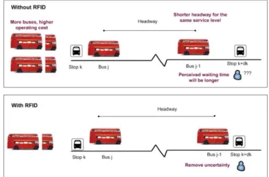
This proposed information system would provide benefits for both the passengers and the bus operators. For passengers, the system will enable better prediction on bus arrival schedule, and subsequently reducing the waiting time and travel time. In addition, although the perceived waiting time is greater than the actual waiting time, the real-time location information of the buses can instigate the perceived to be equal to the actual one, which in turn increases the level of satisfaction from passengers.
For the bus operators, the objective is to manage the dispatch of buses effectively to meet the passenger service requirement reflected by the length of the headway. With the real-time bus location information, bus operators will be able to improve their operation by varying bus schedules to meet unexpected situations. More importantly, as passengers can learn more accurately the arrival time of the buses, the frequency of the buses will not need to be as high to meet the same level of passenger service requirement. In other words, with the real-time bus location information, it is possible that a longer headway can still result in the same average waiting time and the same satisfaction level for the passengers. Therefore, the information acquisition and distribution system will either enhance the customer service level and/or reduce the operation cost for the bus operator. These benefits can be illustrated in Figure 2 below.
Figure 2. RFID application benefits in public transportation
3 Minimum-Cost Headway Model
In this section, a model which captures the total cost of the system for the justification of the RFID application in public transportation is proposed. By comparing the minimum-cost headway for the system using RFID technology with the one without, the amount in cost reduction can be obtained.
Such reduction can then be used as the basis for the justification of RFID implementation. The model is formulated and discussed in the following.
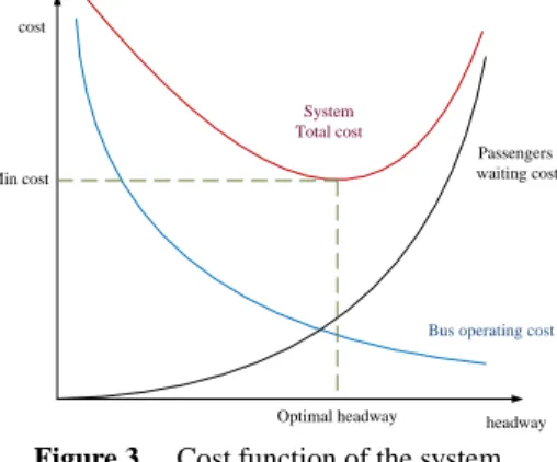
The aim of this model is to find the optimal headways respectively for the two systems. As the bus headway becomes shorter, the service level to passengers increases. However, simultaneously the operating cost for bus operators increases too, because by which it means dispatching a larger number of buses for the same period of time. In contrast, if the headway becomes longer, the number of buss dispatched will be smaller. The passenger waiting time will then be longer and the service level lower.
Such relationship can be illustrated in Figure 3 below.
Figure 3. Cost function of the system
The objective function of the model is the minimization of the system‟s total cost (CT), which consists of operator cost (Co) and passenger cost (Cw), that is,
CT =Co + Cw (1)
The operator cost per day is equal to the bus operating cost (p) multiplied by the vehicle service hours per day. The bus operating cost can be estimated from fuel cost, wage rate, maintenance expenses, and the depreciation of the bus. Vehicle service hours per day is the ratio of the average round trip running time E[t] to the average headway E[h] multiplied by total service hours per day T, that is,
Co = (2)
The passenger cost per day is equal to the passenger waiting cost q multiplied by the perceived waiting time, total ridership per unit time R and total service hours per day T, where the perceived waiting time is the perceived waiting time coefficient multiplied by the average waiting time , which gives
(3)
Understanding the relationship between perceived waiting time and actual waiting time is important. In this model we use perceived waiting time coefficient to compare both dimensions of waiting time.
Hess et al. (2004) did a survey with the bus riders on the duration they usually wait to board the bus. The result of the survey shows that the passengers perceived their average waiting time to be 11.1 minutes. However, the observed average waiting time was 5.8 minutes. Therefore, they proved the hypothesis that the bus riders perceived their wait time to be almost twice what it actually is.
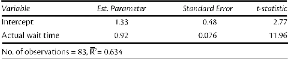
Another research by Mishalani et al. (2006) surveyed 83 passengers over a period of approximately one year, and built a simple linear regression model for the perceived waiting time wp:
wp = β0 + β1a + ε (4)
where a is the actual waiting time, β0 is the parameter representing the intercept of the regression line, β1 denotes the parameter representing the slope of the regression line, and ε is a random variable with a zero mean. The result of their observation again proves that the perceived waiting time is greater than the actual. The result of their observation is shown at the table below:
headway cost
Bus operating cost Passengers waiting cost System
Total cost Min cost
Optimal headway
Table 1. Estimation result of perceived and actual waiting time
The passenger waiting cost can be estimated by wage rate per unit time. Based on a previous research, the value of bus waiting time was estimated between US$8.5 and US$18. Furthermore, most studies reported that passengers value their waiting time at half of their wage rate per hour (Avineri, 2004). However, the function of the waiting cost with respect to time is not that certain, as occupation, travel time to destination, and many other social aspects of the passenger will affect the value of waiting time. (Utility function.)
Basic assumptions of the model are as follows:
1. Arrival of passenger at a bus stop is assumed to be random
2. For the system with the information, perceived waiting time is assumed to be the same as the actual one.
3. Every bus will experience the same condition during the trip, the running time is stochastic; and as soon as the bus arrives at the terminal station, it will return to the starting station along the same route.
4. No limit on bus capacity and bus fleet size. For any optimal headway decision, the buses are ready to be operated.
For the passengers arriving randomly at a stop, the probability density function (p.d.f.) of the waiting time can be estimated by the p.d.f. of the headway on a specific bus route; and the relationship is given as below (Larson et al. 1981):
(5)
where is the probability density function of the waiting time, is the probability density
function of the headway, FH(t) is its cumulative distribution function, = 1-FH(t),
E[h] is the mean headway, and is the bus frequency where . Furthermore, the mean of the waiting time can be calculated as:
(6)
Marguier et al. (1984) gave the direct result of the mean waiting time as:
(7)
where varH is the variance of the buses headway.
Each trip is a stochastic process with the p.d.f. of the bus service time in one route being r(t). Therefore, the mean running time per trip will be given as:
(9)
The system total cost can then be obtained by putting together operator costs and passenger costs, and with h as a decision variable, it can be formulated as follows.
min E[Tc│h] = . T (10)
where h > 0. Solving the objective function, we can get the system total cost and optimal headway for the system with RFID and the one without. The difference between the two costs can then be derived as the benefit of using RFID in the system.
Furthermore, the verification process should be followed by Cost-Benefit Analysis which is the process of measuring the trade-off between the total cost required for RFID investment and the benefits derived from the project. This is a fundamental and indispensable step, because it is the main analysis behind a “go” or “no-go” decision. The cost for implementing RFID technology consists of direct costs and indirect costs. Smith (2000) suggested taking these six main sources into account: the tag itself, the application of the tags to the products, the purchase and installation of the tag readers, the systems integration, the personnel training and reorganization, and the implementation of application solutions. This analysis can be formulated as a return on investment value, as follow:
ROI =
(11)
When the analysis resulted in the feasible return on investment, the operator can confidently implement RFID application in their system.
4 Numerical Example
To illustrate the benefit of the proposed RFID systems, we apply the minimum-cost headway model to a simple case, where the passengers arrival is assumed to follow Poisson process, bus operating cost p is 600 NT/hour, waiting cost q is 300 NT/ hour, the mean ridership R is 150 persons per hour, perceived waiting time coefficient μ is 2 for non-RFID system and the total service time a day is 18 hours. The running time is assumed to follow Normal distribution with mean 60 minutes and standard deviation is 5 minutes. The probability density function of the running time will be:
(12)
The bus arrival is stochastic, and assumed to follow Poisson process, thus VarH= ) and Ew(t)
= E[H]=h. We also assume that the waiting cost is directly proportional with the waiting time, where k
= 0, and the equation (10) will be:
min E[Tc│h] = (13)
The assumption of random passenger arrival is valid for short headway. Previous observations of bus passenger arrivals suggested that random passenger arrivals are valid for 12 minutes headway or less.
In this example, we use 15 minutes headway as the maximum constraints, and we found that the proposed system will have lower system total cost and longer headway.
Table 2. Cost function comparison
Parameter Without RFID With RFID
System total cost 373679.2 NT/day 264275.5 NT/day
Headway 7 minutes 10 minutes
In addition, sensitivity analysis was conducted in order to investigate the system cost model robustness and understand the positive or negative influence of particular model parameters. We used different value for particular parameters; operating cost, waiting cost, passenger ridership and the perceived waiting time coefficient, and the results are as follows:
Table 3. Sensitivity analysis
Value Without RFID With RFID Cost
(NT/day)
Headway (minutes)
Cost (NT/day)
Headway (minutes) Cw 150
264275.5
10 186839.6 14
450 458459.1 6 323594.3 8
Cp 300 264275.5 5 186839.6 7
900 458391.5 8 323594.3 12
λa 75 264275.5 10 186839.6 14
300 528550.9 5 373679.2 7
μ 1.25 295514.4 9
264275.5 10 1.5 323594.3 8
1.75 350054.2 7
It is shown that although we change the parameter to the lower or higher value, the system with RFID always have lower system cost and longer headway. Furthermore, when we change the perceived waiting time coefficient, the system with RFID also performs better.
附件二:
ABSTRACT
With accelerating technological changes and market expansion of electrical and electronic products (EEPs) during last decade, much focus and effort have been placed on the waste of such products. In order to reduce their negative impact on the environment and humans, at the end of their product lifecycles, their wastes need to be properly handled, processed, disposed, and if applicable, remanufactured, recycled or reused. Based on the analysis of the end-of-life EEPs reverse logistic network and the characteristics of its planning, this paper presents a recycling network which has a cost minimization model for the multi-products reverse logistic system. The monetary factors considered in the proposed model include the costs of collection, treatment, and transportation as well as sales income with different fractions of returned products. The proposed optimization model can help to determine the optimal facilities and the material flows in the network. In addition, sensitivity analysis of the model is also presented. Finally, a numerical example is described so as to gain a better insight into the proposed model.
Keywords: Recycling, Reverse Logistics, Recycling Network, Reverse Supply Chain, Electrical and Electronic Equipments, RFID.
1. Introduction
Accelerating technological changes and market expansion of EEPs are making electronic products obsolete very quickly, leading to a significant increase in waste EEPs (WEEPs). According to Environmental Protection Agency (EPA), there are 20 to 50 million metric tons of WEEPs are generated worldwide every year, comprising more than 5% of all municipal solid waste. Developing countries are estimated to triple their output of WEEPs by 2010. In the US alone, some 14 to 20 million personal computers are thrown out every year. In Western Europe, 6 million tons of WEEPs were generated in 1998 and the amount of WEEPs is expected to increase by at least 3-5% per annum.
By 2010, the European Union will be producing around 12 millions tons of electrical and electronic waste annually [1]. It was estimated that about 1.6 million obsolete EEPs were generated in 2003 in China with TV accounting for nearly half of the total [Liu et al., 2006].
WEEPs are a non-homogeneous and complex in terms of materials and components. Many of the materials are highly toxic (Dimitrakakis et al., 2009; Hicks et al., 2005), as well as WEEPs have high residual value (e.g. Iakovou et al., 2009; Nnorom and Osibanjo, 2009; Kumar and Putnan, 2008;
Truttmann and Rechberger, 2006; Kang and Schoenung, 2005) [He et al., 2006; Achillas et al., 2010].
In view of the negative effects of WEEPs on the environment, humans, and the valuable materials that can be reused in them, legislations in many countries have focused their attention on the management of WEEPs, and new techniques have been developed for the recovery of WEEPs. In particular, the European Union (EU) adopted the 2002/96/EC and 2002/95/EC (Restriction of Hazardous Substances- RoHS directive), which causes essential changes in the field of electronic scrap recycling [12,13].
Producers are requested to finance the collection, treatment, recovery, and environmentally sound disposal of WEE. The directive imposes a high recycling rate for all targeted products. The directive imposes a high recycling rate of all targeted WEEPs. Reuse, recycling and recovery rates ranging from 50% to 80% according to the category of equipment considered, must be achieved by producers of EEPs [He et al., 2006].
The recycling of WEEPs is an important step of the end-of-life strategies for WEEPs treatment.
Although there is an increasing amount of research on material recycling models and specific products (Russell et al., 1974; Kroon and Vrijens, 1995; Thierry et al., 1995; Huttunen and Anne, 1996;
Spengler et al., 1997; Nagel and Carsten, 1997; Krikke, 1998; Barros et al., 1998; Ammons and Realff, 1999; Newton and David, 2000; Nunes et al., 2009; Reynaldo and Jurgen, 2009), as well as reverse logistics networks (Spengeler et al., 1997; Rogers and Tibben-Lembke, 1999; Fleischmann et al., 2000;
Salema et al., 2006; Willianm et al., 2007; Demirel, and Gökçen, 2008; Mutha and Pokhare, 2009;
Reynaldo and Jurgen, 2009; El-Sayed et al., 2010; Kannan, 2010), studies specifically addressing WEE products problems (Krikke et al., 1998; Jayaraman et al., 1999; Lee, 2000; Fleischmann et al.,2000;
Deepali, 2005; Rahimifard, 2009; Grunow and Gobbi, 2009; Geraldo and Chang, 2010; Achillas et al.,
2010; Jang and Kim, 2010) are rare or still limited to some specific areas of WEEPs reverse logistics.
In view of lack of in-depth with respect to WEEPs reverse logistics operations in the literatures, this paper presents a recycling network for multi-products reverse logistic system as well as to analyze the material and component flows of returned products at treatment and final stage particularly so that the cost of the recycling can be achieved effectively. The factors considered in the proposed model include the cost of collection, treatment, sales income as well as transportation cost with different fractions of returned products. The proposed model is solved by an algebraic modeling package AMPL (A Mathematical Programming Language).
2. Reverse Logistic Model
Reverse logistics is the collection and transportation of used products and packages [24]. Various researchers categorize and classify the reverse logistic process differently. Fleischmann et al. (2000) categorized recovery into collection, inspection/separation, re-processing, disposal and re-distribution.
Liu et al. (2002) and He et al. (2006) defined recovery process as a combination of re-use, service, re-manufacture, recycle, and disposal, where as Thierry et al. (1995) divided recovery into repair, refurbish, remanufacture, cannibalize, and recycle. Bereketli et al. (2010) showed that re-use, recycling, and disposal are generally three different ways of treating WEE. These alternatives can be explained as follows:
Re-use is the second-hand trading of products for use as originally designed. Re-useable parts can be removed from the product, returned to a manufacturer where they can be reconditioned and assembled into new products [2]; Recycling (with or without disassembly) includes the treatment, recovery, and reprocessing of materials contained in the used products or component in order to replace the virgin materials in the production of new goods [10]; Re-manufacturing is the process of removing specific parts of the waste product for further reuse in new products [10]; Disposal is the processes of incineration (with or without energy recovery) or landfill [10].
In this paper, the proposed model is a formulation for the reverse logistics network design problems. The network is a multi-period multi-echelon, where it consists of collection sites, disassembly sites, treatment sites (recycling centre and repairing centre), final sites (disposal facility, primary and secondary market), as shown in Fig. 1. The objective of the proposed model is to minimize the total cost of the system including transportation cost, processing, operation cost, and disposal costs. Locations of each site are collection, disassembly, treatment, and final sites.
Disassembly Collection
Recycling
Repairing
Disposal
Primary Market
Secondary Market
Waste/disposal items
Directly reuse components Sub-assembly
Faulty components
Hazardous/non- recyclable
materials
Recovery materials
Renewable components
Returned products
Fig.1. Flow of returned products in recycling model
Reverse flow starts with the collection of the used products. Returned products are received from collection points such as retailers, permanent drop-off sites by classified groups. They are then transported to disassembly site. At disassembly sites, the returned products are separated into fractions and determine which components (or parts) are transported to recycle, remanufacturable, repairable, and disposal. Besides, compressing the fractions is also done through disassembly site. Therefore, the volume of waste will be reduced and smaller, it lets all transportation vehicles with full load. The treatment sites which include repairing facilities and recycling facilities are received components from disassembly site. Faulty and old components will be treated at repairing facilities. In recycling facilities, the following typical fractions can be separated in different ways: plastics, ferrous metal fractions are used in iron smelters; most non-ferrous metals go to copper smelters, aluminum smelters, and lead smelters; they can be recycled to become generated material, hazardous materials such as americium, mercury, and lead acid batteries will be sent to special landfills or processing. Final sites encompass disposal facilities, secondary markets and primary markets. The generated materials will be delivered to primary markets and the hazardous or non-recyclable materials will be sent to disposal facilities while the secondary markets include directly reuse components and renewable components.
At collection points, to enhance the efficiency of logistic operations in collection facilities, Radio Frequency Identification (RFID) technology is suggested to manage the information of returned products at collection points in this paper.
Transportation of used or returned goods is probably the most main issue in reverse logistics. In recycling system, returned products need to be physically moved from the end-user to a point of future exploitation. In many cases transportation costs largely influence economic viability of product recycling system. At the same time, it is the requirement of additional transportation that is often conflicting with the environmental benefits of recovery goods. Therefore, careful design and control of adequate transportation systems are crucial in reverse logistics. For recycling, there are three kinds of typical products that lead to three different situations in considering the volume of recycled products.
The first type, like books the product volume still remains the same. The second type reduces the product volume such recycling plastics because some of plastic parts can be compressed into smaller one. The third type makes the volume increase because goods are disassembled into many fractions or components that need more space, for example recycling automobile. In this paper, recycling WEEPs is also third type. When a returned product is sent from collection site to disassembly site its volume and weight are not changed. However, in the following stages, the total volumes of product maybe change. For instance, at disassembly sites the returned product is disassembled into components, materials or fractions that lead to change goods measure as well as product weight.
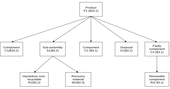
Giving product P1 as a simple example is to describe the variation of the transportation cost and the amount of each type more clearly. Figure 2 shows a disassembly tree of product P1. Product P1 at disassembly sites is received from collection sites. Its transportation cost is 20 dollar per unit and the quantity of product is 1 unit. For component C1, it is a frame of product so the volume is equal to the original volume, although the weight is less than product P1. It is still be charged by the volume, which is 20 dollar and it has 1 unit. At the disassembly sites, product P1 is disassembled into five parts. In case of sub-assembly S1, component C2, disposal D1, faulty component C3, they are charged by weight and the amount of each type is different. For sub-assembly S1, they generate hazardous materials and recovery materials which will be sent to recycling facility for further treatment or sent to disposal facility. The transportation cost of these two types of material is also charged by weight. And faulty component C3 is considered as the same sub-assembly S1.
Component C1($20,1)
Product P1 ($20,1)
Component C2 ($4,1) Sub-assembly
S1($4,2)
Disposal D1($2,1)
Faulty component
C3 ($3,1)
Renewable component
R2( $3,1) Hazardous /non-
recyclable R1($2,2)
Recovery material M1($2,3)
Figure 2. Disassembly tree for product P1
The mathematical model with provides all of the above mentioned decisions and its formulation are presented below.
3. Formulation of the model
The various assumptions considered in the proposed model are described below:
1. The model is a multi-echelon multi-returned products;
2. The collection and final sites are fixed in this model;
3. The capabilities of disassembly, repairing, recycling facilities are limited;
4. The unit of transportation cost is linearly related to distance;
5. Cost parameters (fixed, material, operation, transportation, recycling, disassembly, and disposal costs) are known for each location.
6. The holding cost, storage cost and shortage cost are not considered.
The indices used in the proposed model are described as follows:
: index of collection sites , 1,... ;
c c C
: index of disassembly sites , 1,... ;
d d D
: index of recycling facilities, 1,... ;
l l L
: index of repair facilities, 1,... ;
f f F
: index of disposal facilities, 1,... ;
k k K
: index of secondary market facilities, 1,... ;
r r R
: index of primary market facilities , 1,.... ;
p p P
: number of product types;
m
d: number of sub-assembly components;
m
l: number of faulty components;
m
f: number of directly reuse components;
m
r: number of disposal components;
m
k: number of renewable components;
m
h: number of recovery materials;
m
p: number of non-recyclable materials;
m
q: individual types of returned product, component and material.
S
vThe parameters used in the model are defined as follows:
: the number of components or materials of type is produced from every product type , for , ;
mj
v
A j m
j m S
: the unit transportation cost for different products, components or materials , ;
m v
C m S
: the distance between collection site to disassembly facility ;
D
cdc d
: the distance between disassembly facilitiy to recycling facility ;
D
dld l
: the distance between recycling facility to disposal facility ;
D
lkl k
: the distance between disassembly facilitiy to disposal facility ;
D
dkd k
: the distance between disassembly facility to repair facility ;
D
dfd f
: the distance between repair facility to secondary facility ;
D
frf r
: the distance between recycling facility to primary facility ;
D
lpl p
: the distance between disassembly facility to secondary facility ;
D
drd r
: the operation efficiency at recycling facilities;
l: the operation efficiency at repair facilities;
f: the fix costs of building and operation of a disassembly facility;
f
d: the fix costs of building and operation of a recycling facility;
f
l: the fix costs of building and operation of a repair facility;
f
f: represents the demand of secondary market for component
D
rmr m
f1....
h
l1....
r ;
m M M M M
: represents the demand of primary market for component or material
D
pmp m
v
1,... where , product types
1,...., where , S is sub-assembly components 1,..., where , is directly reusable components
1,..., where For
d d d v
d l l d l
l r r l r v
r k
m M M m S is
m M M M M m
m M M M M m S
m M M M
f
v
, is disposal components
1,...., where , is faulty components
1,...., where , is renewable components
1,...., where , S is recovery material
k r k v
k f k f v
f h h f h v
h p p h p
M m S
m M M M M m S
m M M M M m S
m M M M M m
s 1,..., where , is non-recyclable materials
p q q p q v
m M M M M m S
m M
h
1....M
p ;
: maximum capacity of handing product at disassembly site , , 1... ;
dm d
G m d d D m M
: maximum capacity of handing product at recycling facility , L, 1.. ;
lm d l
G m l l m M M
: maximum capacity of handing product at repair facility , , 1... ;
fm k f
G m f f F m M M
: The unit cost of disposal component and non-recyclabe material for U
m
r 1... k
p 1... q
;m M M M M
: the operation cost of product at disassembly site , , 1... ;
dm d
O m d d D m M
: the operation cost of product at recycling facility , , 1.. ;
lm d l
O m l l L m M M
f
: the operation cost of product at repair facility , , 1...
and the revenues from directly reusable component, recycled or repaired type
1... M 1... 1.... ;
fm k f
l r h h p
O m f f F m M M
m
m M M M M M
: the demand at collection site c for returned product , , .
cm v
b m c C m S
The decision variables involved in this paper are described below:
X
cdm: the amount of products m at collection site c is transported to disassembly site d,X
dk m: the amount of components m at disassembly site d is transported to disposal facilities k,X
dlm: the amount of components m at disassembly site d is transported to recycling facilities l,X
dfm: the amount of components m at disassembly site d is transported to repair facilities f,X
drm: the amount of components m at disassembly site d is transported to secondary market facilities r,X
frm: the amount of components m at repair facilities f is transported to secondary market facilities r,X
lpm: the amount of components m at recycling facilities l is transported to primary market facilities p,X
lk m: the amount of components m at recycling facilities l is transported to disposal facilities k,Y
d : 0-1 variable,Y
d=1 represents building disassembly facility at d otherwiseY
d= 0,Y
l: 0-1 variable,Y
l=1 represents building recycling facility at l otherwiseY
l= 0,Y
f : 0-1 variable,Y
f =1 represents building repair facility at f otherwiseY
f = 0.The objective function of the model is to minimize the total cost of the entire recycling network.
Total cost = Transportation cost + operation cost +fixed cost + disposal cost – revenue of sell reclaimable and renewable materials and components.
Md
C D
cdm
c 1 d 1 m 1 1 1 1
1 1 1 1 1 1 1 1
1 1
Z X ( ) ( )
( ) ( )
+ ( )
l
d
q k
p r
f
k
D L M
cd m dm dlm dl m lm
d l m M
M M
L K D K D L
lkm lk m m dkm dk m m d d l l
l k m M d k m M d l
F M
f f dfm df m fm
f f m M
Min D C O X D C O
X D C U X D C U f Y f Y
f Y X D C O
1 1 1 1 1
1 1 1 1 1 1
( ) (1)
( ) ( )
h
f
p r
h l
D F F R M
frm m fr m
d f r m M
M M
L P D R
lpm m lp m drm m dr m
l p m M d r m M
X U D C
X U D C X U D C
Subject to:
1
for , 1... (2)
D
cdm cm d
d
X b c C m M
Constraint (2) makes sure that all returned products leave the collection site. This means input and output balance of product m at the collection site c.
1 1 1
for , 1.... (3)
Md
C R
cdm mj drj l r
c m r
X A X d D j M M
Md
C
c 1 m 1 1
for , 1... (4)
K
cdm mj dkj r k
k
X A X d D j M M
c 1 1 1
for , 1... (5)
Md
C L
cdm mj dlj d l
m l
X A X d D j M M
Md
C
c 1 m 1 1
for , 1.... (6)
F
cdm mj dfj k f
f
X A X d D j M M
D
d 1 1 1
for , 1... (7)
l
d
M P
dlm mj l lpj h p
m M p
X A X l L j M M
1 1 1
for , 1... (8)
l
d
D M K
dlm mj lkj p q
d m M k
X A X l L j M M
d 1 1 1
for , 1.... (9)
f
k
D M R
dfm mj f frj f h
m M r
X A X f F j M M
Constraints (3), (4), (5) and (6) mean the incoming flow of returned products at the disassembly site d multiple
A
mj is equal to the outgoing flow from disassembly site to secondary market, disposal site, primary market respectively.Constraints (7) and (8) make sure that the incoming flow of returned products at the recycling facility l multiple
A
mjand operation efficiency is equal to the outgoing flow from recycling facility to primary market, disposal site, respectively. Constraint (9) ensures the outgoing flow from the secondary market is equal to the incoming flow of returned products at the repairing facility multiple
A
mj and operation efficiency
D drm
d 1 1
X for , 1.... (10)
D
drm rm l r
d
X D r R m M M
1 1
for , 1... (11)
F F
frm frm fm f h
f f
X X D r R m M M
1 1
for , 1.... (12)
L L
lpm lpm pm h p
l l
X X D p P m M M
Constraints (10), (11), (12) make sure that the amount of components and recovery materials can not exceed the demand for primary market and secondary market.
C
c 1
for , 1.... (13)
cdm dm d
X G d D m M
D
d 1
for , 1.... (14)
dlm lm d l
X G l L m M M
D
d 1
for , 1.... (15)
dfm fm k f
X G f F m M M
, , , , , ,
,0 , , , , , , , (16)
cdm dkm dlm drm frm lpm dfm lkm
X X X X X X X X c d k l r p m f
, , , , , , , , , , , , , , integers (17)
c d l f k p r m C D L F K P R
, , : binary , , (18)
d l f
Y Y Y d l f
Constraint (13) means the amount of returned products sent from collection site c to disassembly site d cannot exceed its maximum capacity; Constraint (14) ensures that the units received by recycling facilities l from disassembly site d cannot exceed its maximum capacity; Constraint (15) limits the unit which is sent from disassembly site d to repairing facilities f to the capacity of repairing facilities f; Constraint (16) means all decision variables are non-negative;
Constraint (17) ensures all indices of returned products, collection site, disassembly site, recycling facilities, repairing facilities, and final sites are integer; Constraint (18) means whether the disassembly facility at point d, recycling facility at point l, repairing facility at point f is built or not.
國外差旅心得報告
於九十九年四月前往美國奧蘭多參加 2010 IEEE International Conference on RFID 國際研討會。2010 IEEE International Conference on RFID 於九十九年四月 十四日至四月十六日舉辦三天,其首屈一指的 RFID 相關研究領域技術交流會議 為最重要的國際研討會之一。
無線射頻辨識系統(RFID)是一個令人興奮的、快速增長的、跨學科領域 的新興技術和應用。此會議出席者為來自世界各地的從業人員和工業界及學術界 之對於 RFID 關注的專業人士,且跨越眾多學科。IEEE RFID 2010 是一個分享及 時 RFID 技術及其應用在各領域研究成果的機會。
在現今產業分工日趨精密下,專業物流中心逐漸成為供應鏈中不可或缺的重 心,除了傳統的實體配送之外,物流中心更將其服務延伸至資訊收集與分析、包 裝、產品維修與客戶服務等領域,提供客戶更高的附加價值。然而於此同時,伴 隨而來的是更多的挑戰,包括日益增多的庫存品項與訂單數量、繁複的庫存變動、
更多元的資訊流動以及日趨激烈的成本競爭,凡此種種使得今日的物流中心必須 尋求更有效的管理方法以及最新的資訊科技以提升競爭力。相對於傳統的自動資 料收集技術,無線射頻辨識(RFID)具有無須人工的自動化資料辨識、可批次 處理多筆物件辨識、無須人工的目視辨識(None-Line-of-Sight)與資料輸入,使 企業在進貨點收、庫存盤點、出庫作業等地方有顯著的效益提昇,其自動化的入 庫、出庫、盤點以及物流交接環節中的 RFID 資訊採集實現物品庫存的透明化管 理;同時並可將標籤作為資料載具,藉由將資料寫入標籤中,隨時紀錄並更新資 料,這些都是傳統的條碼技術所無法比擬的優點。
透過應用 RFID 於物流中心的進貨作業、庫存管理與出貨作業可以有效地降 低人工成本、提升作業準確率並縮短作業時間,進而強化物流中心的整體營運效