國立臺灣大學電機資訊學院電機工程學系 碩士論文
Department of Electrical Engineering
College of Electrical Engineering and Computer Science National Taiwan University
Master Thesis
結合知識資訊與圖像問答之人機互動技術於智慧機器人應用 Human-Robot Interaction Using Knowledge-Based Visual Question Answering System for Intelligent Service Robotics
温郁承 Yu-Cheng Wen
指導教授:羅仁權 博士 Advisor: Ren C. Luo, Ph.D.
中華民國 109 年 7 月 July 2020
致謝
就讀碩士班的這兩年過得非常充實,每一次修課、研究或比賽都是我寶貴的經 驗,總是能在其中體驗到新的樂趣以及不同的挑戰。
首先我要特別感謝我的指導教授羅仁權教授。在羅仁權教授的領導下,我們實 驗室提供了良好的實驗空間以及各種機器人,能在就學期間先接觸到業界等級的 硬體設備實在是難能可貴的經驗,使我能夠充分地將理論與實務接軌,並熟練各種 模擬與操作機器人的方式。同時羅仁權教授也很看重學術論文的研討,學術研究最 避諱地就是閉門造車,必須將眼光一直放在該領域的最前線,才有可能向上做出卓 越的研究,以此為根基羅仁權教授積極鼓勵我們同儕之間分享論文以及將研究內 容撰寫成論文發表於國際會議或期刊,唯有這樣的環境下才有辦法跟上科技的快 速發展,並完成本篇論文。
接著我要感謝實驗室中的其他夥伴,這條路絕對不是單獨一人的精神力與意 志力能夠走完的。感謝實驗室的博士班彭鐿文學長、徐瑋隆學長、蕭東榕學長、于 正倫學長,工程師石崴學長、黃禹軒學長、劉育榕,碩士班徐宇霆以及助理崔雯雅,
不管在任何理論或實作上遇到的困難總是有人能夠一起討論出解決方案,在研究 以外很多實驗室事務也根據學長們的經驗才能夠應對自如。感謝與我同屆的碩士 班李尚倫、HEROBRIXX、許隆銓、葉煥駿,平時分享不同領域的科學新知,以及 比賽或專案時熬夜完成進度,都會是我此生難忘的回憶。
最後要感謝的是我的家人,感謝我的父母能夠尊重我的決定,讓我在一心一意 地完成碩士班的學業,也感謝我的姐姐在我求學不順遂的時候承擔了我一部份的 負面情緒,有家人們在背後支持我才有辦法度過這兩年的時光並且完成這篇研究。
温郁承 謹誌 一百零九年七月
中文摘要
圖像問答(Visual Question Answering)是一個包含電腦視覺和自然語言處理的 多模組任務,其輸入是一張圖和與其相關的自然語言問句,系統必須輸出正確的自 然語言答案。人工智慧系統必須從輸入影像中萃取特徵並轉換這些資訊為合理的 知識來回答問句。
更進一步的研究是由一個具體代理人(embodied agent)來回答問題,也就是 代 理人要在環境中探索並找到與答案相關的圖像線索。由於很多模擬環境可以提供 相片擬真的場景以及可互動的物件,目前大多數的研究都在模擬中進行測試。然而,
當這項技術實際應用在服務型機器人上時有更多可以使用的資訊,其中之一便是 使用者的生活習慣。舉例來說,一台服務型機器人通常一生都在相同的場域內服務,
機器人可以認知使用者經驗和物品習慣擺放位置,例如蘋果通常放在冰箱裡,而冰 箱在廚房的角落等。這些資訊可以幫機器人優化探索環境尋找答案的流程。
這篇論文的目的是將圖像問答落實於服務機器人。我們提出了一個針對具體 代理人系統的記憶性語意式地圖,該地圖會記錄在過去任務序列中探索所產生的 語意式地圖。利用這項序列式的記憶,代理人可以對使用者習慣更加熟悉並完成環 境探索更精簡且有效率。另外同時加入了提前停止機制,根據序列式記憶可以在地 圖上標記出數個關鍵區域,當代理人在這些關鍵區域已有一定程度的探索率,可以 提前結束探索避免多餘的路程。更進一步我們將此系統實際在移動式手臂機器人 上,機器人可以使用導航、操作以及感知能力來完成在環境中進行圖像問答的任務。
我們的實驗顯示使用了記憶型語意式地圖的圖像問答系統比未使用的模型更
加準確,同時在最好的情況可以減少17.4%探索時需要的步數。這樣的結果顯示我
們的方法確實能幫助機器人完成圖像問答任務。
關鍵字: 圖像問答、服務型機器人、語意式地圖、深度學習
ABSTRACT
Visual Question Answering (VQA) is a multi-modal task that includes computer vision and natural language processing techniques. Given an image and a natural language question about the image, the task is to provide an accurate natural language answer. In a such task, the artificial intelligence must extract information from the input image and transform them into reasonable knowledge to answer the question.
An advanced issue is to solve this task by an embodied agent, that is, the agent must explore the environment and find visual clues to answer the given question. Most of the research has implemented this topic in simulated environments as they provide photo- realistic views and interactive environments for real-world scenes. However, there are more information can be obtained as this technique is utilized on service robots. One of them is the habits of users. For example, a service robot usually serves in the same area whole life long. So, it can recognize users’ experience and custom placement of each object, such as the apples are usually in the fridge and the fridge is in the corner of the kitchen. These hints can be used to improve the exploration procedure of finding the answer in the rooms.
The purpose of this thesis is to ground the question answering system to the service robot. We propose a memorial semantic map for an embodied agent system that overlays all the semantic memory in the previous task sequence. Using the sequential memory, the agent can be familiar with the user’s habits and complete the exploration more concisely and efficiently. Also, an early stop mechanism is established. The sequential memory indicates several critical regions that the target object usually appears within the map. As the agent achieves enough high exploration rate of these regions, the exploration procedure can be terminated to avoid redundancies. Furthermore, we implement the
system on a mobile manipulator robot in the real environment. The navigation, manipulation, and perception abilities of the robot make it an appropriate device to operate question answering tasks.
Our experiments show that our question answering system with the proposed memorial semantic map is more accurate than the system without one. With the early stop mechanism, the system can reduce steps by 17.4% in the best case. The result of the real- world implementation shows that our system can help service robots complete visual question answering tasks.
Keywords: Visual Question Answering, Service Robot, Semantic map, Deep learning
CONTENTS
致謝 ... i
中文摘要 ... ii
ABSTRACT ... iii
CONTENTS ... v
LIST OF FIGURES ... viii
LIST OF TABLES ... x
Chapter 1 Introduction ... 1
1.1 Objectives ... 1
1.2 Background ... 2
1.3 Problem Statement ... 4
1.4 Solutions ... 5
1.5 Thesis Organization ... 7
Chapter 2 Question Answering System ... 10
2.1 Embodied Question Answering [2] ... 10
2.2 Interactive Question Answering [4] ... 10
2.2.1 Introduction ... 10
2.2.2 Hierarchical Interactive Memory Network (HIMN) ... 11
2.2.3 Interactive Question Answering Dataset ... 15
2.3 Asynchronous Advantage Actor-Critic (A3C) [5] ... 17
2.3.1 Introduction ... 17
2.3.2 Asynchronous Reinforcement Learning Framework ... 19
2.4 You Only Look Once (YOLO) [6] ... 21
2.4.1 Introduction ... 21
2.4.2 Network Design ... 23
2.4.3 Training ... 24
2.4.4 Inference ... 26
Chapter 3 Memorial Semantic Map ... 29
3.1 Sequential task memory ... 29
3.2 Visualization of Spatial Memory ... 31
3.3 Early Stop Mechanism ... 34
Chapter 4 Robot Specification ... 37
4.1 Introduction... 37
4.2 Manipulator Configuration ... 37
4.2.1 Forward Kinematics Analysis ... 37
4.2.2 Inverse Kinematics Analysis ... 45
4.3 Software Configuration ... 54
4.3.1 Robot Operating System ... 54
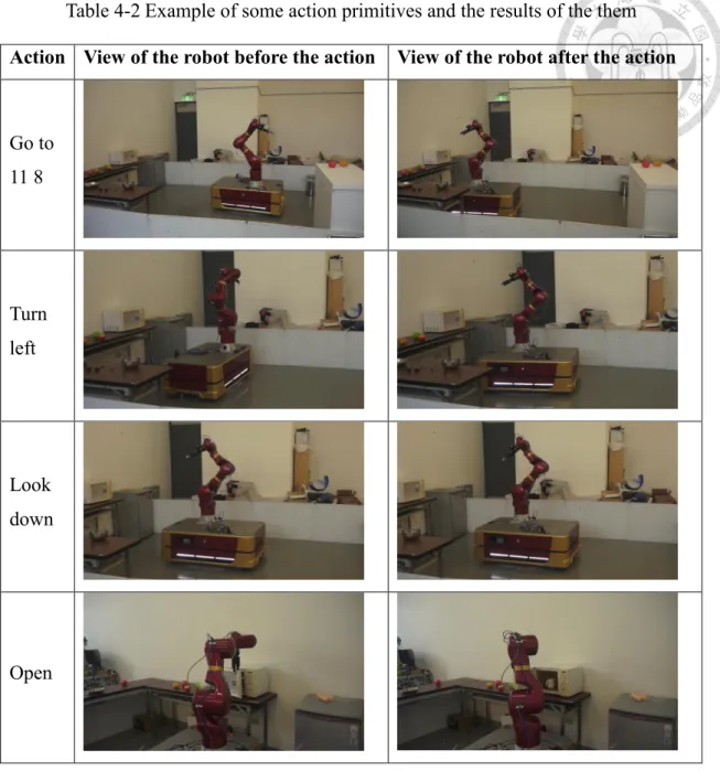
4.3.2 Action Primitives ... 59
Chapter 5 Experiment ... 62
5.1 Introduction... 62
5.2 Simulated Environment implementation ... 62
5.2.1 Introduction ... 62
5.2.2 Dataset Rearrangement ... 65
5.2.3 Comparison Using Reordering IQAUD Testing Dataset ... 66
5.2.4 Ablation Analysis ... 67
5.2.5 Comparison Using Static IQAUD Testing Dataset ... 69
5.3 Real-world Implementation ... 70
5.3.1 Introduction ... 70
5.3.2 Scene Configuration ... 70
5.3.3 Hybrid Object Detection Model ... 74
5.3.4 Mapping, Localization and Navigation ... 78
5.3.5 Full Demonstration ... 81
5.4 Discussion ... 89
Chapter 6 Contributions, Conclusions and Future Works ... 92
6.1 Contributions ... 92
6.2 Conclusions ... 92
6.3 Future Works ... 93
REFERENCE ... 96
VITA ... 99
LIST OF FIGURES
Fig. 1.1 Service robots with manipulators. From left to right is: AMIGO, Care-O-bot
4, TIAGo and Pepper ... 1
Fig. 1.2 Example of free-form, open-ended questions [1] ... 3
Fig. 1.3 The coverage problem proposed by [4] ... 5
Fig. 1.4 An overview of our proposed system ... 6
Fig. 2.1 The complete process of the embodied question answering task ... 10
Fig. 2.2 An overview of the Hierarchical Interactive Memory Network (HIMN) .... 12
Fig. 2.3 Schematic representation of the Planner... 14
Fig. 2.4 Samples from the IQUAD V1 dataset ... 16
Fig. 2.5 The statistics of the IQUAD V1 dataset ... 16
Fig. 2.6 Pseudo code for each actor-leaner thread in asynchronous advantage actor- critic [5] ... 20
Fig. 2.7 The model of YOLO ... 23
Fig. 2.8 The architecture of the network ... 23
Fig. 3.1 Top view of one environment labeled with possible locations of apples ... 32
Fig. 3.2 Top view of one environment labeled with possible location of fridge ... 33
Fig. 4.1 The mobile manipulator robot ... 37
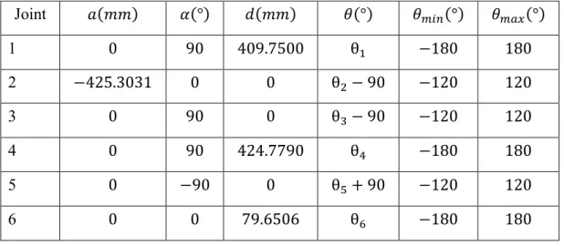
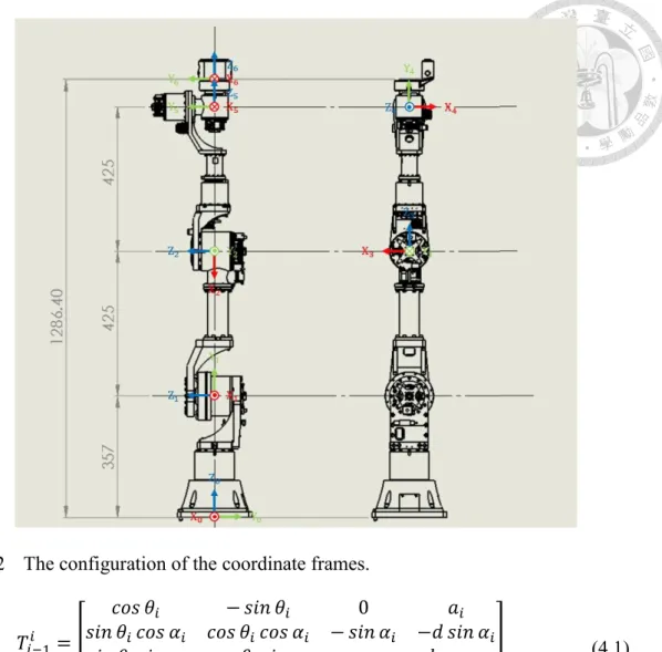
Fig. 4.2 The configuration of the coordinate frames... 40
Fig. 4.3 The user panel of the motion planning tool MoveIt! ... 54
Fig. 4.4 TF structure of the mobile manipulator robot... 57
Fig. 5.1 Example distorted image from RGB-D layout reconstruction ... 64
Fig. 5.2 Example environments from AI2-thor ... 65
Fig. 5.3 The front view of the simulated kitchen ... 71
Fig. 5.4 The side view of the simulated kitchen ... 71
Fig. 5.5 The layout of the simulated kitchen... 72
Fig. 5.6 An overview of the hybrid object detection model ... 74
Fig. 5.7 The metric maps of our scenario ... 79
Fig. 5.8 Two different navigation strategies... 81
Fig. 5.9 The trajectory of the manipulator opens the door of the microwave ... 89
Fig. 5.10 The detection result after the manipulator opens the microwave ... 89
LIST OF TABLES
Table 3-1 Visualization of the memorial semantic map of apples ... 32
Table 3-2 Visualization of the memorial semantic map of fridge ... 33
Table 4-1 Denavit-Hartenberg parameters of the manipulator ... 39
Table 4-2 Example of some action primitives and the results of the them ... 60
Table 5-1 Comparison between different simulated environment. ... 63
Table 5-2 Comparison of the answering accuracy and episode length between different decay factor using reordering IQAUD Testing Dataset ... 67
Table 5-3 Ablation analysis on memorial semantic map and early stop mechanism ... 68
Table 5-4 Activation rate of the early stop mechanism and the corresponding answering accuracy ... 69
Table 5-5 Comparison of the answering accuracy and episode length between different decay factor using static IQAUD Testing Dataset ... 70
Table 5-6 Models for target objects ... 72
Table 5-7 Example 1 of the input image and the detection result of different models . 76 Table 5-8 Example 2 of the input image and the detection result of different models . 77 Table 5-9 Example 3 of the input image and the detection result of different models . 78 Table 5-10 The view of the robot and the corresponding localization result... 80
Table 5-11 Example of answering the question “Is there an apple in the room?” ... 82
Table 5-12Example of answering the question “How many spoons are there in the room?” ... 84
Table 5-13 Example of answering the question “Is there a mug in the microwave?” .... 87
Chapter 1 Introduction
1.1 Objectives
With the rapid development of technology, service robots have become a part of our daily life. For example, you may see robots wander around in the shopping mall and guide purchaser to find their requirements, or shuttle between the counter and tables in the restaurant and send dishes to customers. Robots assist humans by performing tedious, distant, and repetitive tasks, so the user can focus on more complicated jobs. Moreover, some of the service robots are equipped with manipulators, as shown in Fig. 1.1. With the manipulators, the robot can interact with the environment and complete more advanced tasks such as various household chores.
Fig. 1.1 Service robots with manipulators. From left to right is: AMIGO, Care-O-bot 4, TIAGo and Pepper
To interact with the real-world successfully, perception ability plays a key role in obtaining knowledge from the environment. For the raw data, the robot can get RGB image and depth information using an RGB-D sensor, estimate the distance to nearby obstacles using a laser range finder, and record the command of the user using an omnidirectional microphone. The real challenge is how to analyze the environmental data
and extract necessary clues to support the robot to complete the requirements. Hence, investigating the usage of various computer vision and natural language processing techniques on robotics has been a longstanding goal of connecting real-world knowledge with the robot recognition system. For example, a service robot collects RGB images using the front camera and analyzes semantic information within by image segmentation and object detection. Meanwhile, the user can give commands via natural language. The robot parses the syntactic structure and understands the tasks. This is a necessary process for robots to realize real-world information and requirements from users.
1.2 Background
Toward this goal, Visual Question Answering (VQA) [1] is a research topic that draws attention from both computer vision natural language processing communities.
Given an image and a free-form, open-ended, natural language question about the image, the task is to provide an accurate natural language answer, as shown in Fig. 1.2. This task contains feature extraction of physical characteristics and abstract conceptions, such as color or number of the targets and the mental state of a target person. The artificial intelligence requires a vast set of abilities to answer the questions, including fine-grained recognition, object detection, activity recognition, knowledge base reasoning, and commonsense reasoning.
Fig. 1.2 Example of free-form, open-ended questions [1]
In the real case, the robot can get a sequence of images by exploring the environment instead of only one. The research topic had been extended to Embodied Question Answering (EQA) [2], [3]. An answering agent is spawned at a random location in an environment and asked a question related to the environment. The agent can perform primary navigation, such as moving forward and backward, turning left and right, also it perceives information of the surroundings through first-person vision. The goal of the agent is to navigate the environment and gather essential clues to answer the question. In such a task, the system must be proficient in active perception, common sense reasoning, language grounding, and credit assignment.
As the EQA task only considers the mobility, the agent is only able to answer the questions passively. Interactive Question Answering (IQA) [4] deals with the question answering task that requires the agent to interact with a dynamic environment. With the interaction abilities, the agent can explore the map more thoroughly. In addition to the key challenges posed by VQA, an IQA system must be skilled in navigation, manipulation, and execution of a series of actions. As the service robots possess the manipulation and navigation ability, we are more interested in IQA tasks than EQA tasks and the original
VQA tasks. To implement question answering ability on the real robot, we enhance the IQA solving system and transplant it to our robot system.
1.3 Problem Statement
Question answering tasks are the fundamental basis for a service robot to complete various tasks. Firstly, the robot gets instructions from the user using natural language.
Without any manual and translation, the user can command the robot instinctively and conveniently. Next, it explores the environment to collect enough information to complete the tasks, including the position of the essential tools and required target objects. At last, it executes a series of actions to complete the task, such as a household robot cleaning the floor using a mop and a medical robot delivers medicine using a tray. We investigate three basic types of question which is related to environment recognition in the early stage of this research topic, including existence questions (Is there an apple in the kitchen?), counting questions (How many apples are in the kitchen?), and spatial relationship questions (Is there an apple in the fridge?).
Another issue is that most question answering systems with embodied agents are implemented in simulated environments. The room layouts can be rearranged easily by simply modifying the scene or the positions of all objects. In the real case, the arrangement of the rooms might not change drastically and frequently. For example, a service robot usually serves in the same area and environment for long, therefore it can be familiar to the user’s habits such as the placement of dynamic objects or the location of static furniture. This implied feature can help the robot explore the environment more efficiently and precisely. The robot pays attention to places where the target appears regularly and spends less time exploring the ones seldom or never show up.
Moreover, a coverage problem has been discovered by [4]. As shown in Fig. 1.3, the left column is the image taken by the front camera of the embodied agent and the right column is the top view of the environment with the explored path. The given question is
“Is there an egg in the microwave?”. In the first row, the agent found the only target microwave at the early stage of the exploration. However, the agent still tends to increase the exploration coverage rate as shown in the second row. This kind of electrical appliances won’t be move often so the agent can locate them easily if it has semantic memory of the room.
Fig. 1.3 The coverage problem proposed by [4]
1.4 Solutions
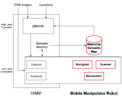
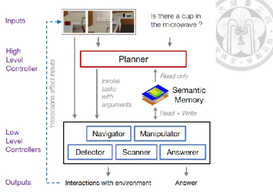
We propose a knowledge-based vision question answering system using the memorial semantic map, as shown in Fig. 1.4. We enhance the Hierarchical Interactive
Memory Network (HIMN) [4] by the memorial semantic map, which records the semantic information of the environment in the previous sequence of tasks. The agent can retain experience from previous tasks, such as the habitual placement of the objects and the fixed pose of the furniture. This experience allows the agent to be more sensitive to the possible positions of the targets. The experiments show that the improved map increases the answering accuracy and decreases the exploration length.
Fig. 1.4 An overview of our proposed system
An early stop mechanism is also induced to terminate the executing task depending on the exploration coverage of the critical regions. A critical region is labeled on the spatial memory as target objects had been detected within it frequently. For the static target objects, such as fridges, cabinets, and microwaves, the agent can stop the exploration when all of the critical regions in the memory are explored. By this mechanism, the agent can avoid increasing the exploration coverage blindly. The agent can be more concentrated on the complete map information and terminates the exploration earlier with an acceptable accuracy drop.
Finally, we implement the proposed system on a mobile manipulator robot. As shown in Fig. 1.4, some of the low-level controllers in the original HIMN, including navigator, scanner, and manipulator, are replaced with the mobile manipulator robot when the system is implemented in the real environment. Our mobile manipulator robot is composed of a differential drive autonomous mobile platform, a 6 degrees of freedom manipulator, and a 2 degrees of freedom gripper. For the sensors, there are two laser range finders mounted in the diagonal corners of the base and one RGB-D camera mounted on the end effector. With the equipment, the robot can perform navigation and manipulation tasks simultaneously, and obtain visual and spatial information using the sensors. These abilities are essential to perform the IQA tasks.
1.5 Thesis Organization
The question answering systems are introduced in Chapter 2. This chapter describes Hierarchical Interactive Memory Network (HIMN) [4], which is the fundamental question answering model, and the kernel module of its controllers, including Asynchronous Advantage Actor-Critic (A3C) [5] algorithm, You Only Look Once real- time object detection (YOLO) [7], and the generation strategy of the original semantic map, which records the result of the object detection during the exploration.
The proposed memorial semantic map is examined in Chapter 3. First, we introduce the overall system architecture that is composed of the enhanced HIMN and our mobile manipulator robot. Then, we explain the concept of the memorial semantic map, including the computation process and the usage of the system. We also propose an early stop mechanism to solve the coverage problem.
We have divided the experiment into two parts in Chapter 5. The first part is
performed in the simulated environment. We compare the proposed system with the origin one, but also discuss the effect of the memorial semantic map and the early stop mechanism by ablation analysis. The second part is implemented in the scene built in our lab. The result shows that our system can help the robot complete question answering tasks in reality. Finally, conclusion, contribution, and future works are described in Chapter 6.
Chapter 2 Question Answering System
2.1 Embodied Question Answering [2]
Embodied Question Answering (EQA) [2, 3] promotes goal-driven agents that can perceive, communicate, and execute actions. As shown in Fig. 2.1, an agent is randomly initialized in the environment and asked a question (“What color is the car?”) about it.
The agent must recognize the surroundings and navigate through rooms to inference the answer (“orange”) to the given question. Compared with Visual Question Answering (VQA), the domain of the question types is refined to object detection, scene recognition, counting, spatial reasoning, color recognition, and logic.
Fig. 2.1 The complete process of the embodied question answering task
Also, the system possesses a hierarchical navigation module that consists of a
‘planner’ that selects actions and a ‘controller’ that execute them. The agent stops navigating after it collects requisite visual information.
2.2 Interactive Question Answering [4]
2.2.1 Introduction
Besides the challenges that visual question answering and embodied question
answering come up with, the agent must interact with the dynamic environment to obtain semantic information actively in this task [4]. A high-level controller is referred to as the planner generates a sequence of actions by choosing and permutating actions from the action primitives, including navigation, detection, manipulation, and answering. The sequence is then executed by a set of low-level controllers which return the control to the planner when their tasks are complete. The cycle of the two-level controllers continues until the agent collects enough information to answer the given question.
2.2.2 Hierarchical Interactive Memory Network (HIMN)
Some question types require the agent to keep track of the objects that have been seen in the exploration along with their locations. For complex scenes with various interactable objects, the agent must hold this information for a long duration. This motivates the need for an explicit external memory representation that is filled by the agent and can be accessed at any time. To address this, [4] proposes the Hierarchical Interactive Memory Network (HIMN) that uses a semantic spatial memory to encode the semantic representation of each location in the scene, as shown in Fig. 2.2. Each location in the memory is composed of a feature vector that encodes the object detection probabilities of different object categories, the free space probability that is a 2D occupancy grid, the coverage that the agent has inspected before, and the navigation intent that the agent has attempted to visit before.
Fig. 2.2 An overview of the Hierarchical Interactive Memory Network (HIMN)
A new recurrent layer formulation, Egocentric Spatial Gated Recurrent Unit (esGRU) is proposed to represent this memory. The esGRU maintains an external global spatial memory represented as a 3D tensor. At each time step, it swaps in local egocentric copies of the memory into the hidden state of the GRU, computes using current inputs, and swaps out the resulting hidden state into the global memory at a predefined location. This speeds up computations and prevents the agent from corrupting the memory at locations far away from its current viewpoint. The agent can access the full memory when navigating and answering questions, which enables long-term recall from observations of the prior states.
Moreover, only the low-level controllers can read and write the memory. Since the planner only makes high-level decisions, it only has the read access to the memory.
The high-level planner triggers the low-level controllers to explore the environment collect information about the given question, and answer the question. This process can be regarded as a reinforcement learning problem that the agent must take a sequence of actions to inference the correct answer. The agent must learn to explore relevant areas of
the scene based on the learned knowledge (e.g. apples are usually in the fridge, fridges are openable, etc.), the current memory state (e.g. the fridge is to the left), the current memory state, current observations (e.g. the fridge is closed), and the given question.
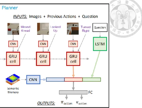
At every time step, the planner chooses one of 32 actions, including to invoke the navigator providing a relative location in a 5 × 5 grids in front of the agent, to invoke the scanner with a direction such as up, down, left and right, to invoke the manipulator with open or close command on the nearby object, or to invoke the answer. This choice is made by producing a policy 𝜋 which consists of probabilities 𝜋𝑖 for each action, and a value 𝑣 for the current state. 𝜋 and 𝑣 are learned using the A3C algorithm [5], which will be introduced in the next section. Fig. 2.3 shows the schematic of the planner.
It consists of a GRU which accepts the current viewpoint (encoded by a CNN) and the previous action. The output of this GRU is combined with the question embedding and the nearby semantic spatial memory embedding to predict 𝜋 and 𝑣. The agent gets a fixed reward or penalty based on whether the answer is correct. Also, the agent receives an intermediate reward for increasing explored coverage of the environment, which effectively trains the network to maximize the amount of the room it has explored. Finally, the planner predicts which high-level actions are available given the current world state at each time step. For example, the agent can’t navigate to some destinations when it is near the wall or it is unable to activate the manipulator when there is no object to interact with. Predicting possible actions at each time step allows gradients to propagate through all actions rather than just the chosen one which leads to higher accuracy and faster convergence.
Fig. 2.3 Schematic representation of the Planner
There are five low-level controllers, including the navigator, scanner, detector, manipulator, and the answerer. The navigator is invoked by the planner which provides the relative coordinate of the target location. Given a destination location and the current estimation of the room’s occupancy gird, the navigator uses A* search algorithm to find the shortest path from the current pose to the goal. As the agent moves through the environment, the navigator applies the esGRU to produce a local (5 × 5) occupancy grid depending on the current visual observations. This local grid map is then updated into the global occupancy estimation and prompts a new shortest path computation. This is a fully supervised problem and can be trained with the standard sigmoid cross entropy. The navigator also invokes the scanner to obtain a wide-angle view of the environment. If the destination is outside the boundary of the room or otherwise impossible (e.g. at the wall or other obstacle), the navigator reports a terminal signal. After the navigator completes the moving process or reports the terminal signal, it returns control back to the planner.
The scanner is a simple controller that changes the view by rotating the front camera up, down, right, or left while keeping the current location of the agent. Then the scanner invokes the detector on the new view.
The detector is a critical component of the model that determines the ability to extract visual information. A YOLOv3 [7] model is fine-tuned on the AI2-THOR [11]
training scenes as a detector. The model can operate at real-time speeds, which is necessary since the detector activates every time step. The detection probabilities are incorporated into spatial memory using the moving average.
The Manipulator is invoked by the planner to manipulate the current state of an object, such as opening and closing the microwave. This leads to a change in the view of the scene. If the object is too far or out of the view, this action will fail.
The answerer is invoked by the planner to answer the question. It uses the current image, the full spatial memory, and the question embedding to predict the answer probabilities ai for each answer candidates of the given question. The question embedding tends to create a tensor with the same size as the spatial memory and the tensor is depth-wise concatenated with the spatial memory to pass through 4 convolutional and max-pooling layers followed by a sum over the spatial layers. The output vector then passes through two fully connected and one SoftMax layer over possible answer choices.
After the answerer is invoked, the task ends.
2.2.3 Interactive Question Answering Dataset
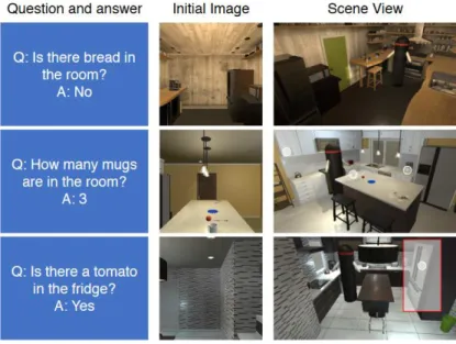
IQUAD V1 (Interactive Question Answering Dataset) is a question answering dataset generated in simulated environment AI2-THOR [11]. It is composed of over 75,000 questions for three different question types, including existence questions (Is there an apple in the kitchen?), counting questions (How many apples are in the kitchen?), and
spatial relationship questions (Is there an apple in the fridge?). Some samples from the IQUAD V1 dataset are shown in Fig. 2.4 and more statistical details are shown in Fig.
2.5. Each question is accompanied by a scene identifier and a unique arrangement of movable objects in the scene. The wide variety of environment configurations prevents the models from creating bias such as “apples are always in the fridge”.
Fig. 2.4 Samples from the IQUAD V1 dataset
Fig. 2.5 The statistics of the IQUAD V1 dataset
To generate these questions, the agent is spawned in a random room with a random configuration and a category of the target object is determined randomly. Then the agent checks the answer from the environment configuration. If the answer is “yes” or greater than zero, the agent has to check if the target objects are findable further. Similar to the
balanced VQA dataset [17], a set of complementary questions is generated to avoid that the agent learns biases in the language instead of the visual modalities. Each question is associated with multiple scene configurations that result in different answers to the question.
The dataset is composed of 30 rooms and split into two subsets, 25 rooms for training and 5 for testing. There are 1024 unique question and configuration pair for each room and question type pair in the training set, and 128 in the testing set. The associated answer is regarded as the ground truth and different models are evaluated using top-1 accuracy.
2.3 Asynchronous Advantage Actor-Critic (A3C) [5]
2.3.1 Introduction
We consider the standard reinforcement learning setting where an agent interacts with an environment ℰ over several discrete time steps. At each time step 𝑡, the agent receives a state 𝑠𝑡 and selects an action 𝑎𝑡 from a set of possible actions 𝒜 according to its policy 𝜋, where 𝜋 is a mapping from the state 𝑠𝑡 to the action 𝑎𝑡. In return, the agent receives the next state 𝑠𝑡+1 and a scalar reward 𝑟𝑡. The process continues until the agent reaches a terminal state. The return 𝑅𝑡 = ∑∞𝑘=0𝛾𝑘𝑟𝑡+𝑘 is the total accumulated return from time step 𝑡 with discount factor 𝛾 ∈ (0,1] . The goal of the agent is to maximize the expected return from each state 𝑠𝑡.
The action value 𝑄𝜋(𝑠, 𝑎) = 𝔼[𝑅𝑡|𝑠𝑡 = 𝑠, 𝑎] is the expected return for selecting an action 𝑎 in the state 𝑠 and following the policy 𝜋 . The optimal value function 𝑄∗(𝑠, 𝑎) = max
π 𝑄𝜋(𝑠, 𝑎) gives the maximum action value for the state 𝑠 and the action 𝑎 achievable by any policy. Similarly, the value of the state 𝑠 under the policy 𝜋 is defined as 𝑉𝜋(𝑠) = 𝔼[𝑅𝑡|𝑠𝑡 = 𝑠] and is simply the expected return for following the
policy 𝜋 from the state s.
In value-based model-free reinforcement learning methods, the action value function is represented using a function approximator, such as a neural network. Let 𝑄(𝑠, 𝑎; 𝜃) be an approximate action-value function with parameters 𝜃 . Updating the 𝜃 can be derived from various reinforcement learning algorithms. One of the algorithms is Q- learning, which aims to directly approximate the optimal action value function:
𝑄∗(𝑠, 𝑎) ≈ 𝑄(𝑠, 𝑎; 𝜃) . In one-step Q-learning, the parameters 𝜃 are learned by iteratively minimizing a sequence of loss functions, where the 𝑖th loss function is defined as
𝐿𝑖(𝜃𝑖) = 𝔼 (𝑟 + 𝛾 max
a′ 𝑄(𝑠′, 𝑎′; 𝜃𝑖−1) − 𝑄(𝑠, 𝑎; 𝜃𝑖))
2
(2.1)
where 𝑠′ is the state encountered after state 𝑠.
The above method is referred to as one-step Q-learning because it updates the action value 𝑄(𝑠, 𝑎) toward the one-step return 𝑟 + 𝛾 max
a′ 𝑄(𝑠, 𝑎; 𝜃𝑖). One drawback of one- step methods is that obtaining a reward 𝑟 only directly affects the value of the current state-action pair 𝑠, 𝑎. The values of other state-action pairs are affected indirectly only through the updated action value 𝑄(𝑠, 𝑎). This makes the learning process slow since many updates are required to propagate a reward to all the relevant preceding states and actions.
One way to propagate rewards faster is by using n-step returns [20][21]. In n-step Q-learning, 𝑄(𝑠, 𝑎) is updated toward the n-step return defined as 𝑟𝑡+ 𝛾𝑟𝑡+1+ ⋯ + 𝛾𝑛−1𝑟𝑡+𝑛−1+ max
a 𝛾𝑛𝑄(𝑠𝑡+𝑛, 𝑎). This results in a single reward 𝑟 directly affecting the values of 𝑛 preceding state-action pairs. This makes the process of propagating a reward to the relevant preceding state and actions much more efficient.
In contrast to the value-based methods, the policy-based model-free methods parameterize the policy 𝜋(𝑠, 𝑎; 𝜃) and update the parameters 𝜃 by performing gradient ascent on the expected return 𝔼[𝑅𝑡] . One classical example of this method is the REINFORCE family of algorithms [22]. The standard REINFORCE updates the policy parameters 𝜃 in the direction ∇𝜃log 𝜋(𝑎𝑡|𝑠𝑡; 𝜃) 𝑅𝑡, which is an unbiased estimation of
∇𝜃𝔼[𝑅𝑡]. It is possible to reduce the variance of this estimation while keeping it unbiased by subtracting a learned function of the state 𝑏𝑡(𝑠𝑡), known as a baseline, from the return.
The resulting gradient is ∇𝜃log 𝜋(𝑎𝑡|𝑠𝑡; 𝜃) (𝑅𝑡− 𝑏𝑡(𝑠𝑡)).
A learned estimation of the value function is commonly used as the baseline 𝑏𝑡(𝑠𝑡) ≈ 𝑉𝜋(𝑠𝑡) leading to a much lower variance estimation of the policy gradient.
When an approximated value function is used as the baseline, the quantity 𝑅𝑡− 𝑏𝑡 used to scale the policy gradient can be seen as an estimation of the advantage of the action 𝑎𝑡 in the state 𝑠𝑡 , or 𝐴(𝑎𝑡, 𝑠𝑡) = 𝑄(𝑎𝑡, 𝑠𝑡) − 𝑉(𝑠𝑡) , because 𝑅𝑡 is an estimation of 𝑄𝜋(𝑎𝑡, 𝑠𝑡) and 𝑏𝑡 is an estimation of 𝑉𝜋(𝑠𝑡). This approach can be view as an actor- critic architecture where the policy 𝜋 is the actor and the baseline 𝑏𝑡 is the critic [23][24].
2.3.2 Asynchronous Reinforcement Learning Framework
The algorithm Asynchronous Advantage Actor-critic (A3C) [5] maintains a policy 𝜋(𝑎𝑡|𝑠𝑡; 𝜃) and an estimation of the value function 𝑉(𝑠𝑡; 𝜃𝑣). The variant of the actor- critic operates in the forward view by explicitly computing n-step returns and uses the mix of n-step returns to update both the policy and the value function. The policy and the value function are updated after every 𝑡𝑚𝑎𝑥 actions or when a terminal state is reached.
The update performed by the algorithm can be seen as
𝛻𝜃′𝑙𝑜𝑔 𝜋(𝑎𝑡|𝑠𝑡; 𝜃′′′) 𝐴(𝑠𝑡; 𝑎𝑡; 𝜃, 𝜃𝑣) where 𝐴(𝑠𝑡; 𝑎𝑡; 𝜃, 𝜃𝑣) is an estimation of the advantage function given by ∑𝑘−1𝑖=0𝛾𝑖𝑟𝑡+𝑖+ 𝛾𝑘𝑉(𝑠𝑡+𝑘; 𝜃𝑣) − 𝑉(𝑠𝑡; 𝜃𝑣) , where 𝑘 can vary from state to state and is upper-bounded by 𝑡𝑚𝑎𝑥. The pseudo-code for the algorithm is shown as Fig. 2.6.
Fig. 2.6 Pseudo code for each actor-leaner thread in asynchronous advantage actor-critic [5]
Note that while the parameters 𝜃 of the policy and 𝜃𝑣 of the value function are shown as separate for generality, they share some parameters in practice. Typically, we use a convolutional neural network that has one SoftMax output for the policy 𝜋(𝑎𝑡|𝑠𝑡; 𝜃) and one linear output for the value function 𝑉(𝑠𝑡; 𝜃𝑣), with all non-output layers shared.
Also, the entropy of the policy 𝜋 is added to the objective function to improve the exploration by discouraging premature convergence to suboptimal deterministic policies.
This technique was first proposed by [26], who found that it was particularly helpful on tasks requiring hierarchical behavior. The gradient of the full objective function including
the entropy regularization term with respect to the policy parameters takes the form
𝛻𝜃′𝑙𝑜𝑔 𝜋(𝑎𝑡|𝑠𝑡; 𝜃′) (𝑅𝑡− 𝑉(𝑠𝑡; 𝜃𝑣)) + 𝛽𝛻𝜃′𝐻(𝜋(𝑠𝑡; 𝜃′)), where 𝐻 is the entropy. The hyperparameter 𝛽 controls the strength of the entropy regularization term.
Three different optimization algorithms are investigated in the asynchronous framework, Stochastic Gradient Descent (SGD) with momentum, RMSProp [25] without shared statistics and RMSProp with shared statistics. The standard non-centered RMSProp update is given by
𝑔 = 𝛼𝑔 + (1 − 𝛼)∆𝜃2 (2.2)
𝜃 ← 𝜃 − 𝜂 ∆𝜃
√𝑔 + 𝜖 (2.3)
,where all operations are performed elementwise. A comparison on the subset of Atari 2600 games showed that a variant of RMSProp where statistics 𝑔 are shared across threads is more robust than the other two methods.
2.4 You Only Look Once (YOLO) [6]
2.4.1 Introduction
The separate components of object detection are unified into a single neural network.
The network uses features from the entire image to predict each bounding box. It also predicts all the bounding boxes across all classes for an image simultaneously. The network reasons globally about the full image and all the objects with it. The design of YOLO enables end-to-end training and real-time speeds while keeping high average precision. The system divides the input image into an 𝑆 × 𝑆 grid. If the center of an object is located in a grid cell, the cell is responsible for detecting the object.
Each grid cell predicts 𝐵 bounding boxes and corresponding confidence scores.
The confidence scores reflect how sure the model is that a cell contains an object and also how accurate the model localized the boxes. Confidence is defined as Pr(𝑂𝑏𝑗𝑒𝑐𝑡) × 𝐼𝑂𝑈𝑝𝑟𝑒𝑑𝑡𝑟𝑢𝑡ℎ. If no object exists in the cell, the confidence score should be zero. Otherwise, the confidence score must equal to the Intersection Over Union (IOU) between the predicted box and the ground truth.
Each bounding box is composed of five predictions, 𝑥, 𝑦, 𝑤, ℎ, and confidence. The (𝑥, 𝑦) coordinates represent the center of the box relative to the bounds of the grid cell.
The (𝑤, ℎ) are the width and height relative to the whole image. The confidence represents the IOU between the predicted box and any of the ground truth boxes. Each grid cell also predicts 𝐶 conditional class probabilities, Pr(𝐶𝑙𝑎𝑠𝑠𝑖|𝑂𝑏𝑗𝑒𝑐𝑡) . These probabilities are conditioned on the grid cell that contains an object. Only a set of the class probabilities are predicted per grid cell, regardless of the number of boxes. At the testing phase, the conditional class probabilities are multiplied with the individual box confidence prediction, calculated by equation (2.4), which gives the class-specific confidence scores of each box. The scores encode both the probability of the class that appears in the box and how accurate the predicted box fits the ground truth. Fig. 2.7 shows the general concept of YOLO.
Pr(𝐶𝑙𝑎𝑠𝑠𝑖|𝑂𝑏𝑗𝑒𝑐𝑡) × Pr(𝑂𝑏𝑗𝑒𝑐𝑡) × 𝐼𝑂𝑈𝑝𝑟𝑒𝑑𝑡𝑟𝑢𝑡ℎ = Pr(𝐶𝑙𝑎𝑠𝑠𝑖) × 𝐼𝑂𝑈𝑝𝑟𝑒𝑑𝑡𝑟𝑢𝑡ℎ (2.4)
Fig. 2.7 The model of YOLO
2.4.2 Network Design
The model is implemented as a convolutional neural network and evaluated on the PASCAL VOC detection dataset [27]. The initial convolutional layers predict the output probabilities and coordinates. The network architecture is inspired by the GoogLeNet model for image classification [28]. It has 24 convolutional layers followed by 2 fully connected layers. Instead of using the inception modules in [28], the network simply contains 1 × 1 reduction layers followed by 3 × 3 convolutional layers, similar to [29].
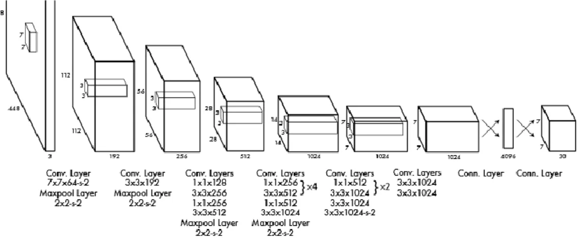
The full network is shown in Fig. 2.8.
Fig. 2.8 The architecture of the network
2.4.3 Training
The convolutional layers are pre-trained on the ImageNet 1000-class competition dataset [30]. For pretraining, the first 20 convolutional layers from Fig. 2.8 is followed by an average-pooling layer and a fully connected layer. The network is trained for approximately a week and achieves a single crop top-5 accuracy of 88% on the ImageNet 2012 validation set, which is comparable to the GoogLeNet models in Caffe’s Model Zoo.
Then the model is converted to perform detection. [31] shows that adding both convolutional and fully connected layers to the pre-trained network can improve the performance. Following this method, four convolutional layers and two fully connected layers are added with randomly initialized weights. The detection process often requires fine-grained visual information, so the input resolution of the network is increased from 224 × 224 to 448 × 448.
The final layer predicts both class probabilities and bounding box coordinates. The width and height of the bounding box are normalized by the width and height of the image to make them be within the range [0, 1]. The (𝑥, 𝑦) coordinates of the bounding box are parametrized to be offsets of a particular grid cell location, so they are also bounded between the range [0, 1]. A linear activate function is used for the final layer and all the other layers use the leaky rectified linear activation calculated by (2.5).
𝜙(𝑥) = { 𝑥 , 𝑖𝑓 𝑥 > 0
0.1𝑥 , 𝑜𝑡ℎ𝑒𝑟𝑤𝑖𝑠𝑒 (2.5)
The sum-squared error is optimized in the output of the model. It is easy to optimize;
however, it does not perfectly align to maximize average precision. It weights the localization error equally with the classification error which may not be ideal. This situation also occurs in the grid cells that do not contain any object. This pushes the
confidence scores of those grid cells towards zero, which often overpower the gradient from the cells that do contain objects. This can lead to model instability and cause the training process to diverge early.
To solve this, the loss from bounding box coordinate predictions is increased and the one from confidence predictions for boxes that don’t contain objects is decreased. Two parameters, 𝜆𝑐𝑜𝑜𝑟𝑑 and 𝜆𝑛𝑜𝑜𝑏𝑗, are used to accomplish this. The Sum-squared error also equally weights errors in large 3 boxes and small boxes. The error metric should reflect that small deviation in the large boxes matters less than the small ones. To partially address this, the model predicts the square root of the width and the height of the bounding box instead of predicting themselves directly.
YOLO predicts multiple bounding boxes per grid cell. At the training phase, only one bounding box predictor is needed to be responsible for each object. One of the predictors is assigned to be responsible for predicting an object based on which predictor has the highest current IOU corresponding with the ground truth. This leads to specialization between the bounding box predictors. Each predictor gets better at predicting specific sizes, aspect ratios, or classes of objects, which improves the overall recall.
During the training phase, the multi-part loss function, calculated by equation (2.6), is optimized, where 𝕝𝑖𝑜𝑏𝑗 denotes if object appears in cell 𝑖 and 𝕝𝑖𝑗𝑜𝑏𝑗 denotes that the 𝑗th bounding box predictor in cell 𝑖 is responsible for that prediction. Note that the loss function only penalizes classification error if an object is present in the grid cell. Also, it only penalizes the bounding box coordinate error if the predictor is responsible for the ground truth box, that is, the predictor has the highest IOU of any predictor in the grid cell.
𝜆𝑐𝑜𝑜𝑟𝑑∑ ∑𝕝𝑖𝑗𝑜𝑏𝑗
𝐵
𝑗=0
[(𝑥𝑖 − 𝑥̂𝑖)2+ (𝑦𝑖 − 𝑦̂𝑖)2]
𝑆2
𝑖=0
+ 𝜆𝑐𝑜𝑜𝑟𝑑∑ ∑𝕝𝑖𝑗𝑜𝑏𝑗
𝐵
𝑗=0
[(√𝑤𝑖− √𝑤̂𝑖)2+ (√ℎ𝑖 − √ℎ̂𝑖)
2
]
𝑆2
𝑖=0
+ ∑ ∑𝕝𝑖𝑗𝑜𝑏𝑗
𝐵
𝑗=0
(𝐶𝑖 − 𝐶̂𝑖)2
𝑆2
𝑖=0
+ 𝜆𝑛𝑜𝑜𝑏𝑗∑ ∑𝕝𝑖𝑗𝑛𝑜𝑜𝑏𝑗
𝐵
𝑗=0
(𝐶𝑖 − 𝐶̂𝑖)2
𝑆20
𝑖=0
+ ∑ ∑𝕝𝑖𝑜𝑏𝑗
𝐵
𝑗=0
(𝑝𝑖(𝑐) − 𝑝̂𝑖(𝑐))2
𝑆20
𝑖=0
(2.6)
The network is trained for about 135 epochs on the training and validation datasets from PASCAL VOC 2007 and 2012. When testing on the 2012 dataset, the VOC 2017 testing dataset is also included during the training phase. The model sets a batch size as 64, a momentum as 0.9, and a decay as 0.0005 during the training phase.
The learning rate schedule is as follows: For the first epoch, the model raises the learning rate from 10−3 to 10−2. If the model starts from a high learning rate, it often diverges due to unstable gradients. Then the model is trained with 10−2 for 75 epochs, 10−3 for 30 epochs, and finally 10−43 for 30 epochs. To avoid overfitting, the model uses dropout and extensive data augmentation. For the dropout, a dropout layer with a dropout rate = 0.5 after the first connected layer prevents co-adaptation between layers [32]. For the data augmentation, the model introduces a random scaling and translations of up to 20% of the size of original images. It also randomly adjusts the exposure and the saturation of the images by up to a factor of 1.5 in the HSV space.
2.4.4 Inference
Just like the training phase, detections for a testing image only requires one of the
network evaluations. The network predicts 98 bounding boxes per image the corresponding class probabilities on PASCAL VOC. YOLO is extremely fast at the testing time since it only requires a single network evaluation, unlike other classifier- based methods. The grid design enforces spatial diversity in the bounding box predictions.
It is often clear which grid cell an object locates in and the network predicts the only one box for each object. However, some large objects or objects near the border of multiple cells can be well localized by multiple cells. Non-maximal suppression can be used to fix the multiple detections.
Chapter 3 Memorial Semantic Map
3.1 Sequential task memory
All of the above-mentioned question answering systems and most corresponding research are proposed in the simulated environment. Some critical issues are usually underestimated in a virtual environment. In this section, we reveal the encountered problems and the corresponding solution using the memorial semantic map.
To test the generality of a model, the spatial memory is reset at the beginning of every test case in the previous research. However, the workspace of an embodied agent can be similar all the time in real-life situations, so the habits of the user can play an important role. If the agent knows the locations where the targets usually deposit ahead, the searching path can be more concise which leads to a decrease in the length of the exploration. Also, the agent can be more determined to these locations, and the question- answering accuracy increases. We propose the memorial semantic map which exponentially overlays all the semantic memory in the previous task sequence. With a proper decay factor, the agent retains general knowledge on the map and is not overwhelmed by the previous experience.
Given a task sequence 𝕋 = {𝑇1, 𝑇2, ⋯ , 𝑇𝑛} , where 𝑛 is the number of the tasks done in the same environment previously, the agent generates a corresponding semantic map sequence 𝕄 = {𝑴𝟏, 𝑴𝟐, ⋯ , 𝑴𝒏} during the exploration, which estimates the positions of objects using the result of object detection and depth estimator. Equation (3.1) shows the structure of the semantic map 𝑴, where 𝑝 is the object detection probability that the requested object 𝑐 appears at the requested position (𝑥, 𝑦).
𝑴[𝑥, 𝑦, 𝑐] = 𝑝 (3.1)
For the current task 𝑇𝑛+1, the semantic map before the exploration is initialized as the memorial semantic map 𝑴𝒏+𝟏∗ . The idea is overlaying all the previous semantic maps in 𝕄 with an exponential decay factor 𝜆m, where 0 < 𝜆𝑚 ≤ 1. Meanwhile, the overlaid result is normalized to preserve probabilistic characteristics. So, the memorial semantic map 𝑴𝒏+𝟏∗ can be calculated by (3.2).
𝑴𝒏+𝟏∗ = ∑𝑛𝑖=1(1 − 𝜆𝑚)𝑛−𝑖𝑴𝒊
∑𝑛𝑖=1(1 − 𝜆𝑚)𝑛−𝑖 = 𝜆𝑚
1 − (1 − 𝜆𝑚)𝑛∑(1 − 𝜆𝑚)𝑛−𝑖𝑴𝒊
𝑛
𝑖=1
(3.2)
Note that if the decay factor 𝜆𝑚 = 1, the memorial semantic map degrades to zero. The agent starts the exploration without any memory and the experiment results can be regarded as a baseline for comparison. Refer to (3.3), if the decay factor 𝜆 approaches 0, the memorial semantic map approaches the average of all the semantic maps in 𝕄. In this case, all of the semantic maps are all equally applied and the old ones might interfere with the agent.
𝜆lim𝑚→0
𝜆𝑚
1 − (1 − 𝜆𝑚)𝑛∑(1 − 𝜆𝑚)𝑛−𝑖𝑴𝒊
𝑛
𝑖=1
= lim
𝜆′𝑚→1
1 − 𝜆′𝑚
1 − 𝜆′𝑚𝑛 ∑ 𝜆′𝑚𝑛−𝑖𝑴𝒊
𝑛
𝑖=1
= lim
𝜆′𝑚→1
𝑑
𝑑𝜆′𝑚((1 − 𝜆′𝑚) ∑𝑛𝑖=1𝜆′𝑚𝑛−𝑖𝑴𝒊) 𝑑
𝑑𝜆′𝑚(1 − 𝜆′𝑚n)
= lim
𝜆′𝑚→1
− ∑𝑛𝑖=1𝜆′𝑚𝑛−𝑖𝒎𝒊
−𝑛𝜆′𝑚𝑛−1 + lim
𝜆′𝑚→1
(1 − 𝜆′𝑚) ∑𝑛𝑖=1(𝑛 − 𝑖)𝜆′𝑚𝑛−𝑖−1𝑴𝒊
−𝑛𝜆′𝑚𝑛−1
=− ∑𝑛𝑖=1𝑴𝒊
−𝑛 = 1
𝑛∑ 𝑴𝒊
𝑛
𝑖=1
(3.3)
3.2 Visualization of Spatial Memory
We visualize the concept of the memorial semantic map. The general idea of the memorial semantic map is to overlay the semantic maps from previous tasks. To generate these maps, the system executes a random sequence of question answering tasks in the same scene with different objects distribution. In the AI2-THOR simulator, the objects can be scattered randomly over several predefined regions. We use this mechanism to randomize the arrangement of the environment, also these regions can be associated with the habitual placements of the object. Before the exploration procedure starts, the system initializes the spatial memory as the memorial semantic map calculated by equation (3.2).
Then the agent explores in the environment and updates the spatial memory by the result of the object detection. Finally, we extract spatial memory after the exploration terminates and transforms the map into a pseudocolor plot.
We extract the memory of two kinds of objects, including the dynamic apples and the static fridges. For the object apple, Fig. 3.1 shows the top view of one of the kitchen scenes and there are four possible regions for it, labeled as A to D. Then the system executes the task sequence and generates the spatial memories. We visualize the resulted map of different decay factor λm = {1.0,0.75,0.5,0.25} , as shown in Table 3-1. As mentioned in section 3.1, if λm is zero, the agent starts the exploration without any memory. Hence, the first column simply shows the result of object detection. In each task, the detection result is involved in all of the maps, so all the graphical feature in the first graph also appears in the others, such as position D in task 1 and position B, C, and D in task 2. The difference between the maps in the same row is the sequential memory part.
Apples show up in position B in task 2 and 3 but not in task 4. This information is recorded on the map with λm< 1.0. As λm increases, the weight of the sequential memory part
also increases and is harder to decay.
Fig. 3.1 Top view of one environment labeled with possible locations of apples Table 3-1 Visualization of the memorial semantic map of apples
Task 𝛌𝐦= 𝟏. 𝟎 𝛌𝐦 = 𝟎. 𝟕𝟓 𝛌𝐦= 𝟎. 𝟓 𝛌𝐦= 𝟎. 𝟐𝟓
T1
T2
T4
T8
For object fridge, Fig. 3.2 shows the top view of the same kitchen scene and the only
possible region is labeled on it. After the exploration procedure of task 1, the fridge is found and the detection result is marked in the spatial memory, as shown in Table 3-1. As the agent always finds the fridge in the following tasks, the sequential memory is updated frequently and the location of the fridge is always kept in the memory. If the target of the task is the fridge, the agent can localize the location quickly.
Fig. 3.2 Top view of one environment labeled with possible location of fridge Table 3-2 Visualization of the memorial semantic map of fridge
Task 𝛌𝐦= 𝟏. 𝟎 𝛌𝐦 = 𝟎. 𝟕𝟓 𝛌𝐦= 𝟎. 𝟓 𝛌𝐦= 𝟎. 𝟐𝟓
T1
T2
T4
T8
In the experiment section, we investigate the effect of different decay factor 𝜆m. With a proper sequential memory, the system can perform the exploration more efficiently.
3.3 Early Stop Mechanism
The agent might be too persistent in increasing exploration coverage. In most cases, this conduces a complete recognition of the environment, but the agent sometimes still wander around as all the existed targets are found in the early exploration. If the targets are the fixed ones, such as fridges and cabinets, the agent can stop at once after all of the target position candidates registered in the memorial semantic map are inspected. We develop the early stop mechanism to detect this kind of situation. Several critical regions are labeled if they are frequently updated and the target objects are detected within. The two conditions mean that the target objects appear in the area recently. If the agent has explored all of the critical regions, the task can be terminated as soon as possible.
Given a task sequence 𝕋 = {𝑇1, 𝑇2, ⋯ , 𝑇𝑛} and the associated semantic map sequence 𝕄 = {𝑴𝟏, 𝑴𝟐, ⋯ , 𝑴𝒏} , the memorial semantic map 𝑴𝒏+𝟏∗ is calculated first using equation (2) before the exploration starts. To activate the early stop mechanism, the agent must make sure that the exploration coverage of the critical region 𝑹 in the memorial semantic map surpasses a predefined threshold 𝜃, that is, all of the possible positions of the target objects have been inspected during the exploration. The critical region is determined by (4), where 𝑘 is a duration constant. The more dynamic the arrangement
of the environment is, the higher the value of 𝑘 must be to increase the size of the critical region. In this case, the early stop mechanism won’t be triggered easily and the agent tends to explore more.
𝑹 = {(𝑥, 𝑦)|𝑴𝒏+𝟏∗ [𝑥, 𝑦, 𝑜] > 𝜆m𝑘} (3.4)
Chapter 4 Robot Specification
4.1 Introduction
We design and build a mobile manipulator robot as shown in Fig. 4.1. The robot is a combination of a differential drive autonomous robot and a 6 degrees of freedom manipulator with a 2-fingers adaptive robot gripper. The robot is equipped with an industrial personal computer that connects with the controllers of the base, the motion controller of the manipulator, the depth camera mounted on the end effector, and 2 laser range finders mounted on the base.
Fig. 4.1 The mobile manipulator robot
4.2 Manipulator Configuration
4.2.1 Forward Kinematics Analysis
To find the pose of the end-effector from the base coordinate of the manipulator, it’s necessary to derive the relationship between them. However, the robot manipulator is a
![Fig. 1.2 Example of free-form, open-ended questions [1]](https://thumb-ap.123doks.com/thumbv2/9libinfo/9604818.630957/14.892.257.785.119.423/fig-example-free-form-open-ended-questions.webp)