國 立 交 通 大 學
電信工程研究所
碩 士 論 文
應用參數化閉合型式並考慮時序相關性的
統計型靜態時序分析於軟性錯誤率分析
Applying Parameterized Closed-Form SSTA
Considering Timing Correlation to Soft
Error Rate Analysis
研究生:張家慶
指導教授:溫宏斌
應用參數化閉合型式並考慮時序相關性的統計型靜態時
序分析於軟性錯誤率分析
Applying Parameterized Closed-Form Considering Timing
Correlation to Soft Error Rate Analysis
研究生:張家慶
Student: Chia-Ching Chang
指導教授:溫宏斌
Advisor:Hung-Pin Wen
國 立 交 通 大 學
電 信 工 程 研 究 所
碩 士 論 文
A Thesis
Submitted to Institute of Communication Enginerring College of Electrical and Computer Engineering
National Chiao Tung University in partial Fulfillment of the Requirements
for the Degree of Master
in
Communication Engineering
July 2011
Hsinchu, Taiwan, Republic of China
應用參數化閉合型式並考慮時序相關性的統計型靜態時序分析於軟性錯誤率分析
學生:張家慶
指導教授
:溫宏斌
國立交通大學電信工程研究所碩士班
摘
要
對於屬於次微米世代的 CMOS 設計,由於製程變異,軟性錯誤的統計特性變得
更為複雜。製程變異使得軟性錯誤的行為有極大的不確定性,因此要精準地估計
電路的軟性錯誤,統計的方法是不可或缺的。然而,不論現有用於軟性錯誤架構
的方法是什麼,這些方法通常需要在效率與準確度之間作取捨。因此在這篇論
文,我們提出以一次標準式為基礎的邏輯閘單元模型,以降低時間耗損。在假設
所有製程變異的參數皆為常態分佈的前提下,這些被推導成閉合形式的單元模型
是精準的。根據這些模型,可以用類似區塊基準統計性時序分析法去分析統計性
軟性錯誤。實驗結果展示了提出的模型只有很小的誤差並且證明了我們的方法可
以極具效率地估計電路上的統計性軟性錯誤,而且對比 SPICE 模擬出的結果是足
夠準確的。
Applying Parameterized Closed-Form SSTA Considering Timing Correlation to Soft
Error Rate Analysis
student:Chia-Ching Chang
Advisors:Dr. Hung-Pin Wen
Institute of Communication Engineering
National Chiao Tung University
ABSTRACT
For CMOS designs in the deep submicron era, statistical methods are essential to
accurately estimate circuit SER under process variations, which lead to significant
uncertainty in behavior of soft errors. Due to process variations, a number of statistical
natures of soft errors become more sophisticated than their static one. However,
regardless of the methods used in current statistical SER (SSER) frameworks are, they
usually require the tradeoff of accuracy and efficiency. In this work, we present
accurate cell models based on a first-order-canonical form to reduce timing cost, and
upon which, SSERs can be analyzed similarly to block-based SSTA. These cell
models are derived in closed-form and precise under the assumption of normal
distribution of process parameters. Experimental results show that the errors of
proposed models are small and our approach is highly efficient for estimating circuit
SSERs with reasonable accuracy when compared to SPICE s imulation.
誌 謝
能夠順利完成這篇碩士論文,首先要感謝的就是我的指導教授溫宏彬老
師。在碩士的兩年,老師不僅在課業與研究上給我許多寶貴的意見與幫助,
在做人處事上,無論是人與人之間的相處之道,或者是處理事情的態度與方
法,更是使我獲益良多。而實驗室的氣氛也因為老師對待學生就像是朋友一
般,因此非常的歡樂與團結。真的很慶幸可以成為老師的學生,讓我在面對
充滿不確定性的未來有足夠的自信心,不管是遇到任何困難也能夠以更具健
全的心理去面對。
接著要感謝的是實驗室的博士班學姊佳伶與千慧,從我進入這間實驗室開
始就不厭其煩地指導我,舉凡 EDA 這個領域的詳細介紹、面臨的問題以及解
決的方法,或者是在寫程式時需有的觀念,讓我得以慢慢地步上研究的軌道。
還有要謝謝學長陳韋廷、高振源、陳彥后和學姊郭雨欣,在我遇到課業、研
究甚至是心理上的挫折時,都會幫助我解決。另外也要謝謝玗璇、欣恬、凱
華、鈞堯、宣銘、昱澤、竣維、鉉威、洧炷這些實驗室的研究夥伴們和女友
嘉珣,有了你們的幫助與鼓勵,讓我在研究之路不會感到無助與孤獨。
最後以此文獻給我最摯愛的父母以及兩個哥哥,感謝你們永遠都在背後默默
地支持我,給予我無限的勇氣與動力,讓我可以完全無後顧之憂地向前邁進。
Contents
List of Figures v
List of Tables vi
1 Introduction 1
2 Preliminary 5
2.1 Statistical static timing analysis . . . 6
2.2 Statistical soft error rate analysis . . . 8
3 Full-Chip Estimation of Statistical Soft Error Rate (SSER) 10 3.1 Soft-Error Accumulation . . . 11
3.2 Logic-Probability Computation . . . 13
3.3 Electrical-Pulse Propagation . . . 14
3.4 Algorithm of SEU propagation . . . 15
4 Parameterized First-Order Canonical Forms for ψhit and ψprop 18 4.1 Construct linear timing models . . . 21
4.2 Parameter estimation . . . 22
4.3 Correlation issue . . . 23
4.4 Re-convergence Handling . . . 24
4.4.1 Derive Width of Re-Convergent transient faults . . . 24
4.4.2 Update Logic Probability . . . 27
5 Experimental Results 28 5.1 Accuracy of Model . . . 29
5.2 Measurement of Full-Chip SSER . . . 32
6 Conclusion 34
List of Figures
1.1 Three masking mechanisms for soft errors . . . 2
1.2 SER differences between static and Monte-Carlo SPICE simulation w.r.t. different process variation . . . 3
2.1 Flow of close-form parameterized block-based SSTA . . . 6
3.1 SSER analysis at full-chip level . . . 11
3.2 Signal probability for one OR gate . . . 14
4.1 SSTA-based method w/o considering correlation between transition signals 20 4.2 Iterative split and merge . . . 23
4.3 Reconvergent Structure . . . 24
4.4 Illustration of same orientation merge operation . . . 26
4.5 Opposite orientation merge operation at a AND/OR gate . . . 26
5.1 Model accuracy of AND . . . 30
5.2 Model accuracy of OR . . . 30
List of Tables
4.1 Comparison of SER w/ and w/o considering correlation between transition
signals . . . 23
5.1 Summary of model error . . . 31
Chapter 1
Introduction
Due to increasingly CMOS technology scaling, the reliability issues become more and more important. When only concerned in memory, soft errors are one of the major failure mechanisms for logic circuits [1]. Compared to the typical failure rate for reliability mech-anisms, the soft error rate (SER) is much higher and has become an unavoidable problem since the circuit speed increases rapidly, which makes occurrence of soft errors more fre-quent [2]. Radiation-induced transient faults result in such errors, which are latched by state-holding elements, and make data state of the elements corrupted without permanently damaging the elements.
The behavioral analysis of soft errors depends on three masking effects [3]: logical, electrical and timing masking. As shown in Figure 1.1, logical masking occurs when the transient faults are blocked during propagation by a controlling value on the side-input of one gate along the propagation path. Due to electrical properties of gates, electrical masking leads to the attenuation or the amplification of transient faults, depending on the input values of gates [23]. Timing masking happens when the transient faults arrive a state-holding element outside or smaller than its clock transition window (setup time + hold time). timing masking Particle hit electrical masking vhigh logical masking Q Q SET CLR D Q Q SET CLR D Q Q SET CLR D
Figure 1.1: Three masking mechanisms for soft errors
Traditional methods to evaluate static soft error for combinational logic were pro-posed. FASER [5] and MARS-C [24] apply symbolic techniques to both logical and electrical maskings and scale the error probability according to the specified clock pe-riod. SERA methodology in [6] computes SER by evaluating error-latching probability and the electrical-masking effect without considering logical masking. Krishnaswamy et al. [13] propose a static analysis for timing masking by backwards computing the prop-agation starting from the error latching windows. SEAT-LA [25] and Rao et al. [26] ob-tain good SER estimation compared to the result of SPICE simulation by simultaneously characterize cells, flip-flops and propagation of transient faults. The work in [12]
propa-gates and electrically evaluates the change of transient faults through one gate according to the logic function and analytical models, which are incorporated with nonlinear transis-tor current. Consequently, SER has become a key metric for circuit reliability and been extensively investigated.
In recent years, process variations have been gradually concerned and brought a new challenge for accurately estimating the SER. The authors in [15] [16] first analyze the impact of the variation sources on SER and find that the traditional static approaches will underestimate circuit SER in presence of process variation. Using 45nm technology, the impact of process variations on SER is illustrated in Figure 1.2, where SERs are measured
on a sample circuit under different process variations (σproc’s). According to Figure 1.2, the
simulation result of SERs by static SPICE is underestimated compared to statistical results. Peng el al. in [23] apply state-of-art statistical learning algorithm to tackle the variation-induced uncertainty and build SVM models for transient faults. Kuo et al. in [14] propose quality table-based cell models to estimate SSER and customize the use of quasi-random sequences to shorten runtime. However, regardless of what approaches used in current SSER frameworks are, they usually need to sacrifice either the efficiency for the accuracy or the accuracy for efficiency.
0 10 20 30 40 50 60 70 0% 1% 2% 5% 10% S E R ( µ F IT )
Process Variation (σproc)
Figure 1.2: SER differences between static and Monte-Carlo SPICE simulation w.r.t. dif-ferent process variation
In this work, we propose a new idea that a transient fault is considered as two transitions, one is a rising edge and the other is a falling edge. Two edges are analyzed separately using analytical approach of statistical static timing analysis [19], which is based on the concept of a first-order canonical form [20]. Since a transient fault is analyzed by a closed-form
statistical timing method, not only a large portion of timing cost can be reduced but the timing information can be preserved, which is helpful to analyze the interactive behavior of transient faults. Moreover, the correlations are the main concerns when applying the SSTA approach to estimate the SSER. From experiment results, we know that the correla-tion between transicorrela-tion signal and corresponding gate delay should be considered but the correlation between transition signals can be ignored instead since the SER difference is smaller than 1%. Thus, we employ the correlation-aware parameterized SSTA to obtain more accurate SER. From the experimental results, our SSER framework is capable of obtaining reasonable results with much better speed compared to previous works.
The rest of this paper is organized as follows: In Chapter 2, SSTA-related and SSER-related works are reviewed. In Chapter 3, we propose the flow of parameterized closed-form framework for SSER analysis. Parameterized First-order canonical closed-form of transient faults is detailed in Chapter 4. Chapter 5 illustrates the experimental results, including the accuracy of our models, the SSERs as well as the runtime over a variety of ISCAS benchmarks and a series of multipliers. Chapter 6 concludes this paper and describes the future works.
Chapter 2
Preliminary
In this section, we review the first order canonical form for statistical timing analysis and the frameworks of statistical soft error rate analysis in section 2.1 and section 2.2, respectively.
2.1
Statistical static timing analysis
Pick one cell c in propagation tree Get moments of both inputs of c
cout = cin1+cin2 or
cout = max(cin1+cin2)
sum operation to compute
the moment of cout
Yes
max operation to derive the
moment of cout Merging connection Appending connection Is the propagation tree empty? Estimate the normal parameters by MME
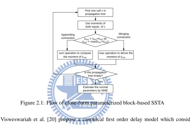
Figure 2.1: Flow of close-form parameterized block-based SSTA
Visweswariah et al. [20] propose a canonical first order delay model which consid-ers both correlated and independent randomness. By expressing timing quantities in the canonical form, the arrival times and required arrival times can be propagated through tim-ing graph ustim-ing a linear time block-based statistical timtim-ing algorithm. Moreover, the local and global criticality probabilities can be computed with a very small timing cost. In a standard or canonical first order form, a timing quantity such as gate or wire delay can be expressed as follows: t , a0+ n X i=1 ai∆Xi+ an+1∆Va
where a0 is the nominal value of delay, ∆Xi represents the variation of n global sources
Xi from their nominal value, ai is the sensitivity of each of global sources of variation,
and ∀i ∈ [1, n]. ∆Va means the variation of an independent random variable Va from its
Then, to apply canonical first order form to statistical timing analysis, the operations of
sumand max are required. The procedure of the sum operation of two distributed-jointly
random variables is described as follows: Let t0 = t + d, where t0 is the resultant by
summing up two mutually-correlated random variablest and d. The mean and variance of
t0 can be derived as:
µt0 = E(t0) = E(t + d)
= E(t) + E(d) = µt+ µd (2.1)
σt20 = E((t0− E(t0))2)
= E(t02) − (E(t0))2
= E((t + d)2) − (E(t + d))2
= E(t2) + 2E(td) + E(d2)
−(E(t))2− 2E(t)E(d) − (E(d))2
= E(t2) − (E(t))2+ E(d2) − (E(d))2
+2E(td) − 2E(t)E(d)
= σt2+ σ2d+ 2ρtdσtσd (2.2)
whereρtddenotes the correlation coefficient oft and d. On the other hand, Visweswariah
et al. [20] use the concept of tightness probability to deduce the result of max operation of two timing quantities in canonical form. To describe the max operation, we denote Z = max(X, Y ), where Z is the responsive random variable obtained by taking max operation between random variables X and Y . The moment of Z can be derived as:
µZ = E(Z) = E(max(X, Y )) = µXTx+ µY(1 − TX) + θφ( µX + µY θ ) σZ2 = µ2(Z) = µ2(max(X, Y )) = (σX2 + µ2X)TX + (σY2 + µ2Y)(1 − TX) +(µX + µY)θφ( µX − µY θ ) − µ 2 Z
larger than random variable Y . More details can be referred to [17] [18].
In the proposed framework, a transient fault is split into two transition signals, which are timing quantities and can be expressed in canonical form so they also can be efficiently analyzed by a parameterized block-based SSTA. The difference between SSER and SSTA is that the prior one only cares about the pulse-width change of a transient fault rather than the timing with maximum delay.
2.2
Statistical soft error rate analysis
Due to process variation, the behavior of a transient fault becomes unpredictable and can be no longer estimated accurately by static approaches. Both learning-based and simulation-based methods for statistical soft error analysis are studied in the literaure.
Peng el al. [23] re-examine the soft error behaviors caused by radiation-induced par-ticles under process variation and find that transient faults are no longer monotonically diminishing after propagation. In other words, both the upgrade and degradation of tran-sient faults are possible. Moreover, they conclude that the traditional static methods will underestimate the soft error rate due to the weak charge-induced soft errors are ignored. Thus, they propose a statistically learning-based framework to cope with these complex and sophisticated issues. The major idea for prediction of the behavior of soft errors is to analyze three masking effects through the start-of-the-art learning theory. Although using learning-based approach to analyze SER can achieve good efficiency, the accuracy of SER results is not good enough.
In their framework [23], the elements of SSER problem can formulated into 1. signal-probability computation
2. electrical-probability computation
where the electrical probability computation includes two effects, timing masking effect and electrical masking effect. And the signal probability computation corresponds to the logical masking effect. Details of the framework will be described in section 3.
Since quality statistical model is the bottleneck of all previous SSER frameworks, sat-isfactory accuracy of SSER results have not yet been achieved. For this reason, the authors
in [14] present accurate table-based cell models for transient fault distributions accord-ing to which a Monte Carlo SSER analysis framework is built. By lookaccord-ing up the pre-characterized table cells, both the sample points of strike and propagation transient faults can be obtained in each iteration, and then the new distributions of strike and propagation models are computed from these points. To shorten the runtime, Kuo et al. [14] further de-ploys a heuristic to customize the use of quasi-random sequences, which successfully speed up the convergence of simulation error. Although the accurate SSER results are gotten in this work, the lengthy simulation time is still unsolved and make this simulation-based method inapplicable to industrial circuits.
The two works described above differ from the methods to derive the distributions of transient faults arriving any primary output or flip flop, which is related to electrical prob-ability computation. In this work, the goal is also to efficiently and accurately compute the final distributions of transient faults, which is a procedure of linear form formulation shown in Figure 3.1. After acquiring the distribution of transient faults, the occurrence of soft errors on the flip-flops can be determined by checking whether these transient faults fall outside or are smaller than the error latching window of the flip flops or not. If a tran-sient fault is wide enough to cover the latching window, a soft error is generated; otherwise, it is masked.
Chapter 3
Full-Chip Estimation of Statistical Soft
Error Rate (SSER)
Logic-Probability Computation More p? Compute SER(p) Sum up SER(p) SERChip Soft-Error Accumulation
Find the distribution of first-strike transient fault Split the transient pulse into
rising and falling signals
Electrical-Pulse Propagation Reach flip-flop? +Δq Block-based propagation of transition signals More charge? Circuit gate-level netlist Estimate signal probability
Pick one hit cell p Pick one charge DWAA correction
No
No
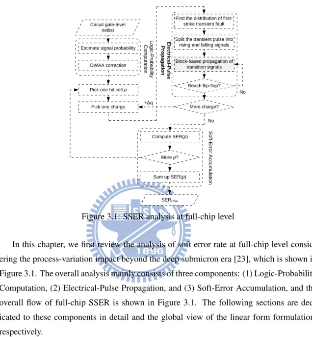
Figure 3.1: SSER analysis at full-chip level
In this chapter, we first review the analysis of soft error rate at full-chip level consid-ering the process-variation impact beyond the deep submicron era [23], which is shown in Figure 3.1. The overall analysis mainly consists of three components: (1) Logic-Probability Computation, (2) Electrical-Pulse Propagation, and (3) Soft-Error Accumulation, and the overall flow of full-chip SSER is shown in Figure 3.1. The following sections are ded-icated to these components in detail and the global view of the linear form formulation, respectively.
3.1
Soft-Error Accumulation
From the full-chip perspective, the overall SER can be defined by accumulating soft
errors (SE(·)) resulting from particle strikes at each individual gate (ci) in the chip. That
SERf ull-chip = #gate
X
i=1
SE(ci)
where #gatedenotes the total number of gates which are possible to be struck by radiative
particles in the chip. Note that the transient fault caused by a particle strike may be prop-agated and received by different memory-holding elements, and results in numerous soft errors.
Each SE(ci) can be further formulated by integrating the products of particle-hit rate
and the error probability over the range of charge strength from qminto qmax as follows:
SE(ci) =
Z qmax
q=qmin
RP H(q) × Prerr(ci, q) dq (3.1)
where Prerr(ci, q) denotes the error probability that a transient fault originated from a
col-lection charge with strength q at node ci can be latched by any flip-flop.
Here RP H(q), the particle-hit rate, is the effective frequency that a particle with strength
q hit at the circuit in unit time and in [3] [6], it is defined as
RP H(q) = F × K × A(ci) × 1 qs × exp(−q qs )
where F , K, A() and qsdenote the constants for neutron flux (> 10MeV), the
technology-independent fitting parameter, the susceptible area in cm2 and the slope of charge
collec-tion, respectively.
One key point that can be observed from the definition is that smaller charge collection occurs much more frequently than large charge collection and accounts for the difference between static SER and statistical SER in [23]. Moreover, for a practical SER analysis framework, the above continuous integration in Equation 3.1 is often simplified by dis-cretization. That is,
SE(ci) =
n X
k=1
RP H(qk) × Prerr(ci, qk) (3.2)
where qk= k × (qmax− qmin)/n and according to [5] and [23], empirically, n = 3 or n = 4
suffices to reach a satisfactory accuracy of SER.
The error probability Prerr(ci, q) depends on all three masking effects illustrated in
Prerr(ci, q) = #F F X
j=1
Prlogc(ci, dj) × Prelec(ci, dj, q) (3.3)
where #F F, Prlogc, Prelec, respectively, denote the total number of flip-flops in the circuit,
the logic-masking probability and the electrical probability related to electrical-masking and timing-masking effects. The corresponding details are elaborated into the following sections.
3.2
Logic-Probability Computation
Prlogc(ci, dj) represents the overall logic probability of successfully propagating the
transient faults through all paths from gate ci to flip-flop dj. A Prlogc(ci, dj) can be
com-puted by multiplying the signal probabilities of non-controlling value of all gates on paths and shown as:
Prlogc(ci, dj) = Prsig(c∗i) × Y
ck∈ci dj
Prsig(ck)
where Prsig(c∗i) is the probability of logic-0 (logic-1) when a positive (negative) transient
fault is generated at ci, and ck, neither ci nor dj, is another gate along the path (ci dj).
Prsig(ck) represents the signal probability for a non-controlling side-input that does not forbid a transient fault propagating through gate ck.
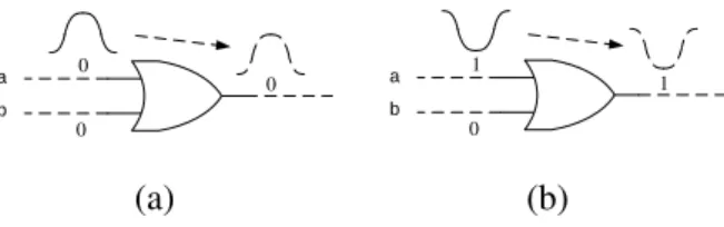
Take Figure 3.2 for example to comput Prsig. Assume the probability of being 1 on
input a is Pa, and so is Pb. The signal requirement for propagating a positive transient fault
is both a = 0 and b = 0 as shown in Figure 3.2(a). Hence, the probability of passing such
an event is Prsig = (1 − Pa) × (1 − Pb). To propagate a negative transient fault as shown in
Figure 3.2(b), the necessary condition is a = 1 and b = 0, so the corresponding probability
is Prsig = Pa× (1 − Pb). Other gate types can be derived similarly.
When computing signal probabilities, it is essential to handle the reconvergent fanout nodes (RFONs) because ignoring RFONs may lead to considerable computation error [21]. However, true signal probabilities may not be always available especially when the num-ber of design inputs exceeds certain bound. Therefore, a linear-time heuristic is typically
0 a b 0 0 0 a b 1 1 (a) (b)
Figure 3.2: Signal probability for one OR gate
employed to handle the RFONs. In this paper, we choose dynamic weighted averaging
algorithm (DWAA)and more details of DWAA can be found in [21].
3.3
Electrical-Pulse Propagation
Prelec(ci, dj, q) in Equation (3.3) reflects the electrical-masking and timing-masking
ef-fects on the transient fault induced by charge q along the path (ci dj) and can be further
decomposed into
Prelec(ci, dj, q) = Prt-mask(pwj, wj)
= Prt-mask(fe-mask(ci, dj, q), wj)
where Prt-mask() and fe-mask() accounts for the timing-masking and electrical-masking
effects, respectively.
Timing-masking probability, Prt-mask(), assumes that the pulse width of an arrival
tran-sient fault and the latching window (tsetup+ thold) of a flip-flop with a clock period are all
random variables and denoted as pw, w, and tclk, respectively. A new random variable v
can be defined as v = pw − w where µv and σv are its mean and standard deviation. Then,
Prt-mask(pw, w) = 1
tclk
Z µv+3σv
0
v × P (v > 0)dv
On the other side, electrical-masking function, fe-mask(), reflects the pulse-width change
of transient faults through a gate and can be defined as:
Given the nodeciwhere the charge with strengthq strikes and causes a transient fault,
propagates along the path ci dj through nodev0, v1,· · · , vn, vn+1 where v0 and vn+1
denote the hit gateci and flip-flopdj, respectively.
fe-mask(ci, dj, q) =
λprop(· · · (λprop(λprop
| {z }
ntimes
(pw0, 1), 2), · · · ), n) (3.4)
wherepw0 = λhit(ci, q) is the initial pulse width induced by a particle with charge q strikes
at gateciand∀k ∈ [0, n), pwk+1 = λprop(pwk, k + 1) represents the resulting pulse width
after propagating throughvk+1.
λhit and λprop in Equation (3.4), respectively, represent the first-hit and propagation
distribution functions, which can reflect the behavior of transient faults during their gen-erations and propagations. Both functions are non-deterministic and can only be
approxi-mated in a SER analysis framework. Accordingly, efficient and accurate models, ψhit and
ψprop, become the most critical since integrating the process-variation impacts on soft error
is difficult . In this work, both ψhit and ψprop are derived as first-order canonical forms
so that deduction over ψhit and ψprop can be done by the method of moment estimation
(MME) [22]. So, the estimated electrical-masking function in Equation (3.4) can be modi-fied into
fe-mask(ci, dj, q) ≈
ψprop(· · · (ψprop(ψprop
| {z }
ntimes
(pwc0, 1), 2), · · · ), n)
wherepwc0 = ψhit(ci, q) and ∀k ∈ [0, n), eachpwck+1 = λprop(pwck, k + 1) is an estimator
for the pulse width after propagating through vk+1along the path (ci dj).
3.4
Algorithm of SEU propagation
Since it is possible that a single event upset (SEU) happens at one of the gates on the circuit under test (CUT), all gates on the CUT are the candidates of hit gate. After the
hit gate ci is determined, the transient fault induced by a particle strike at output of ci
can be analyzed in the generation stage and propagation stage by first-hit model ψhit and
propagation model ψprop, respectively. The pseudocode of the algorithm for electrical-pulse
propagation in Figure 3.1 is described as:
Algorithm 1 SEU at (hitGate ci)
1: markPropagationTree(ci)
2: sortPropagationTreeByLevel
3: repeat
4: Node Z = output of next gate cj in Gprop
5: D = Get Moment(cj)
6: RFON = CheckRFON(Z)
7: if RFON is false then
8: X = on-path input of cj
9: tx= Get moment(X)
10: Tz = sum(D,tx)
11: end if
12: if RFON is true then
13: (X,Y ) = inputs of cj 14: tx= Get moment(X) 15: ty = Get moment(Y ) 16: t0x= sum(D,tx) 17: t0y = sum(D,ty) 18: Tz = merge(t0x,t0y) 19: end if
20: until Visit all nodes in propagation tree
21: return moments of transient faults arriving any flip-flop or PO;
In the generation stage, the first-hit model ψhit is used to deduce the distribution of the
particle-induced transient fault on the output of the hit gate ci. Then, the initial transient
fault is split into a rising-transition signal and a falling-transition signal, denoted as t0
t0f, and their moments can be deduced by ψhit, too. The propagation stage is succeeding to the generation stage and can be described in three steps.
Firstly, to acquire the propagation tree Gpropof the transient fault starting from ci and
terminating at any pseudo primary output (PPO) or any primary output (PO), the breath-first search is employed to trace all the gates on Gprop. Once a gate is visited, it will be added
into Gprop and the flag is set as VISITED so that any gate on the reconvergent nodes won’t
be tranced again. After Gprop is built, all gates in Gprop are ranked by their topological
orders and then analyzed using parameterized closed-form SSTA in order.
In the next step, the initial transition signals t0r and t0f are propagated along Gprop by
the propagation model ψprop in a block-based way. During propagation, two conditions
are handled in different ways. For the case that a reconvergent fanout node (RFON) is on the output pin of the current gate cj, sum and merge operations are deployed to deal with the issue of convolution of transient faults. For the opposite case, only sum operation is required during propagation.
In the final step, the transient faults arriving at any PPO or any PO are reconstructed by
merging tr and tf and the combined pulse-width distributions are used to compute SER,
Chapter 4
Parameterized First-Order Canonical
Forms for ψ
hit
and ψ
prop
Traditional Monte-Carlo methods for SSER analysis are known to suffer from long simulation time to derive pulse-width distributions for particle strikes and transient-fault propagation. Instead, in this paper, we employ a parameterized first-order canonical form to derive the two distributions. We simply divide a transient-fault into two transition sig-nals (rising and falling), and each signal can be analyzed by statistical static timing analysis (SSTA). Accordingly, the rising and falling transitions are modeled as two normally
dis-tributed random variables, tr and tf. Moreover, the first-hit and propagation distribution
functions, ψhit and ψprop, can be expressed into the form as follows,
ψ : ~x → ~y
where ~x denotes a vector of input variables and ~y denotes a vector of target values. ~x
provides guidance to find the target ~y in the models and includes several relationships of
electrical and physical properties between cells and transient faults.
For example, the width of a transient pulse hitting at one output of a cell decreases as the capacitance of the output loads of the cell increases (because the charging/discharging time of capacitors increases). Another example is that the hitting charge with greater strength
causes the wider transient pulse. Hence, for first-hit model ψhit, ~x includes the charge
strength, the type of driving gate and output loads; ~y contains mean and variance of initial
pulse-width, correlation coefficient and slopes of the two transitions. Similarly, for ψprop,
~
x consists of the same components as ~x in ψhit with an additional component-the slope of
the transition signal; ~y contains the transition slope, mean and variance of gate delay,
cor-relation between transition signal and the corresponding gate delay, and between transition signals.
From the proposed idea, a random variable pw denoting the width of a particle-induced transient pulse can be decomposed into two jointly normally distributed random variables:
the rising transition tr and the falling transition tf, and can be computed as:
pw = (
tf − tr if the pulse is positive
tr− tf if the pulse is negative (4.1)
Based on ψhit and ψprop, both tr and tf are then analyzed by a parameterized SSTA
variable µpwand σpwwith the estimatorsµbpwandbσpw. The overall analysis flow is outlined as follows:
1. Transient-fault generation and decomposition: At first, first-hit model ψhit() is used to estimate the distribution of the initial pulse width pw0. Then the estimated pulse
widthpwc0 is factorized into two initial transitions t0
r and t0f according to the ratio of
their slopes.
2. Block-based propagation: The two timing signals keep updated by ψprop() once being
propagated through one gate to reflect the gate delay. The step repeats until both the rising and falling signals arrives at any PO or PPO.
3. Pulse-width reconstruction: Once both signals reach any PO or PPO, they are merged to reconstruct a new transient pulse to determine whether a soft error occurs. The reconstruction step exercises the proposed idea as Equation (4.1).
To take Figure 4.1 for example, the original transient pulse generated by a particle strike at G0 is split into two transition signals, and then the two signals start their propagation individually. Finally, both two signals end at G2 and are merged to reconstruct the transient pulse.
particle hit Propagation
split merge G0 G1 G2 Q Q SET CLR D
Figure 4.1: SSTA-based method w/o considering correlation between transition signals
Details of each step are organized as: After introducing the first-hit model and propa-gation model in section 4.1, the distributions of width of a transient fault is estimated by MME in section 4.2. Then the issues of reconvergence and correlations are discussed in section 4.4 and 4.3, respectively.
4.1
Construct linear timing models
In the first step, ψhit() is responsible for approximating the means and variances of t0r
and t0f and the corresponding computations can be enumerated as:
µt0 r = 0 µt0 f = µpwc0 σt20 r = σ 2 t0 f × τ 0 r/f σt20 f = σ 2 c pw0/(1 + (τr/f0 )2− 2τr/f0 × ρt0 rt0f)
where the superscript is the corresponding topology order originated from the hit cell G0, τ0
r/f means the slope ratio defined as the slope of the rising signal to that of the falling
signal, and ρt0
rt0f is the correlation coefficient of t
0
r and t0f and pre-characterized into a table.
After obtaining the distributions of the two initial transition signals, the linear timing model
ψprop() is deployed to propagate both signals to primary outputs.
The derivation of the linear timing model ψprop() computed by a typical statistical static
timing analysis is given as: a transition signal t arrives at an input of a gate with delay d, and t and d can be expressed in the linear closed-form as
t = t0+ n X i=1 ai∆Xi+ an+1∆Va and d = d0+ n X i=1 bi∆Xi+ bn+1∆Vb
Here t0 and d0 are the nominal values for t and d, respectively. ∆Xi is the variation of n
global sources from its nominal value; ai and bi, respectively, represent the sensitivities of
the transition signal and gate delay to each of ∆Xi. Both ∆Vaand ∆Vbare variations of the
independent random variable Vaand Vbfrom their mean value, and their timing sensitivities
are denoted as an+1and bn+1, respectively.
After the timing signal t passes through the gate, the output timing signal t0 is updated
as t + d, and thus we can deduce t0 by a sum operation of two jointly normally distributed
tinf at a gate input can be propagated to the gate output and modeled by the linear timing model ψprop. Then the output timing signals become
toutr = tinr + dr (4.2)
toutf = tinf + df (4.3)
where subscripts r and f represent rising and falling, respectively, and the superscript (input or output) represent the pin locations.
Since we have deduced the first-hit model ψhit() and the propagation model ψprop(),
the pulse width of a transient fault can be approximated by Equation (4.1). The details are provided in the following section.
4.2
Parameter estimation
Given the first-hit model ψhit() and the propagation model ψprop(), the final distribution
ofpw in Figure 4.1 can be further expended according to Equation (4.1). That is,c
c pw = t2f − t2 r = (t1f + d2f) − (t1r+ d2r) = (t0f + 2 X i=1 dif) − (t0r+ 2 X i=1 dir) (4.4)
where the superscript is the corresponding topological order originated from the hit node.
So, the mean and variance of pw can be calculated by performing a series of sumc
operations over transition signals and corresponding gate delays. To derive the general form of a transient pulse, which is generated at one hit cell at mth level and propagated to one flip-flop at nth level, we generalize Equation (4.4) and rewrite it into:
c pw = tn−mf − tn−m r = (t0f + n−m X i=1 dif) − (t0r+ n−m X i=1 dir) (4.5)
4.3
Correlation issue
Correlation is a major concern when using the first-order canonical-form based SSTA
to approximate the behavior of transient pulse. It is because the pair of transition signals tr
and tf are mutually dependent instead of completely uncorrelated. Intuitively, the solution
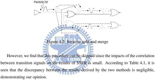
for the issue is to iteratively split and merge the transient faults during propagation. As
illustration in Figure 4.2, a transient pulse is reconstructed by merging tr and tf once both
the transitions pass through a cell, and then split again in order to be propagated towards successive cells.
Particle hit
Figure 4.2: Iterative split and merge
However, we find that this procedure can be skipped since the impacts of the correlation between transition signals on the results of SSER is small. According to Table 4.1, it is seen that the discrepancy between the results derived by the two methods is negligible, demonstrating our opinion.
Table 4.1: Comparison of SER w/ and w/o considering correlation between transition sig-nals
circuit SSERssta(a) SSERrecon.(b) Diff.(%)
(µFIT) (µFIT) (b−aa )
c17 5.627E02 5.628E02 1.78E-02
c432 2.2818E05 2.2814E05 -1.82E-03
c2670 8.003E04 8.003E04 6.62E-04
4.4
Re-convergence Handling
The number of transient faults are doubled if there is a reconvergent structure along propagation path in the circuit, resulting in the complexity of the SSER analysis increases exponentially. As shown in Figure 4.3, a particle hits the output of G0 and induces a transient pulse. Then, the transient faults propagate along the paths in a block-based way and finally reconverge at the inputs of U0 and U1. Consequently, two positive transient faults appear on the output of U0, and two transient faults with different directions appear on the output of U1.
Particle hit
G0
U0
U1
Figure 4.3: Reconvergent Structure
To resolve this reconvergence problem, we propose a two-stage approach. At the first stage, these transient faults are classified into two groups according to their orientations. Then the outcomes of the pulse width and the logic probability of these convoluted transient faults are derived at the second stage. In the second stage, the pulse-width distribution of convoluted transient faults is derived by two newly defined merge operations and the logic probability is updated as the union of the ones associated with these transient faults.
4.4.1
Derive Width of Re-Convergent transient faults
The motivation to define new merge operations for two timing signals is that the pulse-width result of transient faults will be underestimated if we adopt traditional one (max) to deduce the result of these convoluted timing signals and the reason is discussed later.
The idea for merging multiple positive transient faults can be defined as:
merge(pw1, pw2, · · · , pwn) =
merge(tf 1, · · · , tf n) + merge(tr1, · · · , trn) (4.6)
The merge operation with multiple (>2) operands like Equation (4.6) is computed by
taking the 2-operand merge iteratively. Let t0 = merge(t1, t2), t1 and t2 follow normal
distribution, and the result t0does, too.
merge(t1, · · · , tk) = merge(merge(t1, t2), · · · , merge(tk, tk+1))
= merge(t1,bk
2c, td k 2e,k)
= t1,k (4.7)
The 2-operand merge can be further classified into two types to deduce convoluted pulses with the same orientations and with opposite directions.
To derive the pulse width of reconvergent transient faults with the same orientation, we define the same-orientation merge operation as a worst-case operation that the new pulse is composed of the latest transition signal and the earliest transition signal among these reconvergent transient faults. Take Figure 4.4(a) for example. We denote the later
transient fault and earlier transient fault as P1 and P2, respectively. The result of
same-orientation mergeoperation performed on P1and P2 should be the latest transition and the
earliest transition among them, respectively denoted as tr1 and tf 2. However, the result
derived by traditional max operation will be tr2 and tf 2, leading to an underestimation for
the pulse-width result of the reconvergent transient faults. Same conclusion is also obtained in Figure 4.4(b).
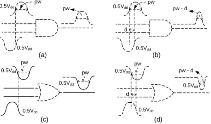
Before performing same-orientation merge operation over two reconvergent transient faults, the existence of overlapping should be checked. As shown in figure 4.4(a), if over-lapping happens, the earliest edge and the latest edge will be chosen to form the a pulse; otherwise, the width of the new transient fault is the sum of the two convoluted transient faults, as displayed in figure 4.4(b).
On the other hand, for the reconvergent transient faults with opposite orientations, the result of pulse width is determined by the interactive behavior of them. Take Figure 4.5
particle hit P1 P2 (a) particle hit pw1 pw2 pw1 + pw2 (b)
Figure 4.4: Illustration of same orientation merge operation
for example. if the positive transient fault appearing at one input of a AND gate does not overlap the negative transient fault appearing at the other input of the AND gate, the pulse-width result is just the pulse-width of the positive transient fault pw since the negative transient fault is forbidden by the controlling value on the side-input. If the overlapping occurs, the result is computed as the width of positive transient fault pw minus the overlapping part among positive and negative transient faults d due to the negative transient fault masks the part of positive transient fault. Other gate types can be derived similarly.
It is worthy to notice that due to the timing informations of transition signals are pre-served, the issue of reconvergence can be analyzed in such way which is unavailable for in traditional SSER methods [23] [14].
(c) (d) 0.5Vdd 0.5Vdd 0.5Vdd 0.5Vdd d pw pw - d pw pw 0.5Vdd 0.5V dd (a) (b) 0.5Vdd 0.5Vdd 0.5Vdd 0.5Vdd d pw pw - d pw pw
4.4.2
Update Logic Probability
The logic probability at reconvergence fanout nodes should be updated to reflect the reconvergence phenomenon. For convoluted transient faults, the result of logic probability is the union of the ones of these transient faults since this condition is equivalent to that all these transient faults can pass through the reconvergent node. The same result is obtained for the transient faults with the opposite orientation.
Chapter 5
We implement the proposed framework in C/C++ and exercise on a Linux machine with Intel(R) Core(TM) i7 processor and 16G RAM. To extract the delay characteristics of each gate type, we perform Monte-Carlo SPICE simulation on 4 small benchmark circuits from [23] with a 45nm Nandgate Open Cell Library [36] as the 45 nm cell library.
The method for training these delay data of each gate type can be summarized in three steps: in step 1, all the gates along the propagation path are randomly selected after the path is generated; in step 2, the number of loadings composed of randomly selected gates is arbitrarily chosen for each gate on the propagation path; and in the final step, the charac-teristics of the transient faults induced by radiation particles with various charge strength are extracted by performing Monte-Carlo SPICE simulation. After obtaining these sim-ulation results, we group them according to the charge strength of radiation particle, the transition slope, and the output loadings.
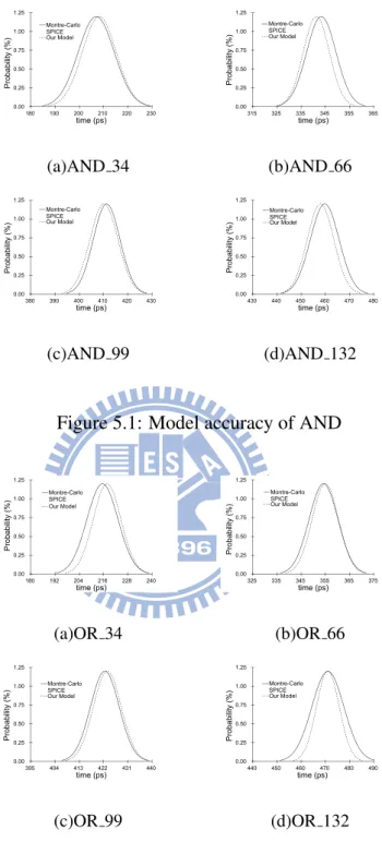
Model errors of a AND gate and a OR gate are summarized in Figure 5.1 and Figure 5.2, respectively, and the average model errors of each gate type are shown in Table 5.1. All the results of overall SSER of circuits are built on ISCAS85 benchmarks and a series of multipliers. Considering the extremely long runtime of Monte Carlo SPICE simulation (w / 100 runs), we can only afford to perform tests on small circuits with the largest one containing 26 gates, 31 striking nodes and 5 inputs.
5.1
Accuracy of Model
Figure 5.1 and 5.2 compare the PDF results of transient faults induced by four particles with different charge strength of proposed models and the ones of Monte-Carlo SPICE for one AND gate and one OR gate, respectively. In Figure 5.1 , it can be seen that all the comparison of PDF results exist small mean differences except for Figure 5.1(b) which has little larger mean error. All the comparison of PDF results shown in Figure 5.2 present the very small mean discrepancies except for Figure 5.2(a) which has a little larger mean error. The variances of the PDF result derived by the proposed method in both figures are not close to the ones derived by Monte-Carlo SPICE. The reason is discussed later.
0.00 0.25 0.50 0.75 1.00 1.25 180 190 200 210 220 230 Pro b a b ili ty (% ) time (ps) Montre-Carlo SPICE Our Model 0.00 0.25 0.50 0.75 1.00 1.25 315 325 335 345 355 365 Pro b a b ili ty (% ) time (ps) Montre-Carlo SPICE Our Model (a)AND 34 (b)AND 66 0.00 0.25 0.50 0.75 1.00 1.25 380 390 400 410 420 430 Pro b a b ili ty (% ) time (ps) Montre-Carlo SPICE Our Model 0.00 0.25 0.50 0.75 1.00 1.25 430 440 450 460 470 480 Pro b a b ili ty (% ) time (ps) Montre-Carlo SPICE Our Model (c)AND 99 (d)AND 132
Figure 5.1: Model accuracy of AND
0.00 0.25 0.50 0.75 1.00 1.25 180 192 204 216 228 240 Pro b a b ili ty (% ) time (ps) Montre-Carlo SPICE Our Model 0.00 0.25 0.50 0.75 1.00 1.25 325 335 345 355 365 375 Pro b a b ili ty (% ) time (ps) Montre-Carlo SPICE Our Model (a)OR 34 (b)OR 66 0.00 0.25 0.50 0.75 1.00 1.25 395 404 413 422 431 440 Pro b a b ili ty (% ) time (ps) Montre-Carlo SPICE Our Model 0.00 0.25 0.50 0.75 1.00 1.25 440 450 460 470 480 490 Pro b a b ili ty (% ) time (ps) Montre-Carlo SPICE Our Model (c)OR 99 (d)OR 132
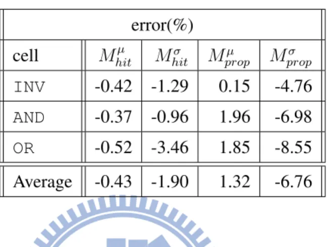
first column lists the cell libraries, and the following four columns denote mean and vari-ance errors of first-hit model and propagation model, respectively. The average mean and variance errors of our first-hit model are all less than 2%, and so are the average mean error of propagation models.
Table 5.1: Summary of model error error(%)
cell Mhitµ Mσ
hit Mpropµ Mpropσ
INV -0.42 -1.29 0.15 -4.76
AND -0.37 -0.96 1.96 -6.98
OR -0.52 -3.46 1.85 -8.55
Average -0.43 -1.90 1.32 -6.76
The reason why the variance errors of propagation model is worse is that the shape of hitting pulse is changed during propagating and become hardly predictable. As shown in Figure 5.3, the sinusoidal shape of a hitting pulse will be transformed into trapezoid, and the variance of flat part of trapezoid shape can not be properly described by the proposed idea, leading to little larger variance errors.
1 1
1
10 times of INV
Figure 5.3: Explanation of model error
The following section demonstrates the effectiveness of the proposed idea by compar-ing the results derived by our approach and the ones obtained from Monte-Carlo SPICE simulation.
5.2
Measurement of Full-Chip SSER
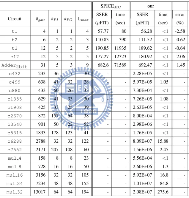
Information of all benchmark circuits is listed at Table 5.2. The name of each circuit is shown in column 1, containing 3 circuits from [23], ISCAS85 benchmarks and a series of multipliers with various bits. The following four columns denote the number of gates, the number of primary inputs (PI), the number of primary outputs, and the max topological level, respectively. For all circuits, each node under every input pattern combination is
injected with four levels of electrical charges: Q0 = 34f C, Q1 = 66f C, Q2 = 99f C,
Q3 = 132f C, where Q0 is the weakest charge capable of generating a transient fault under
the settings in the experiments.
We compare the results of Monte-Carlo SPICE simulation with the results of proposed framework on t1, t2, t3, c17, and Adder2bit, and the comparisons of the measured values of SSER and the required runtime are shown in the next four columns. All errors of t1, t2, t3, c17, and Adder2bit are all less than 3%, demonstrating that the pro-posed idea can achieve reasonable accuracy with very low timing costs. Besides, the result of Adder2bit is accurate even if it contains many RFONs, demonstrating our reconver-gence handling is effective.
More results of SSER analysis on a variety of circuits are also shown in Table 5.2. The runtime remains small even if the circuit size becomes big. Moreover, because the proposed idea is built upon a parameterized closed-form blocked-based SSTA, the longer logic depth will induce longer runtime. c6288 and all multipliers (mul 16 to mul 32) consume slightly more time due to such reason.
Table 5.2: SSER measurement of various benchmark circuits
SPICEM C our
Circuit #gate #P I #P O Lmax
SSER time SSER time error
(µFIT) (sec) (µFIT) (sec) (%)
t1 4 1 1 4 57.77 80 56.28 <1 -2.58 t2 6 2 2 3 110.83 390 111.52 <1 0.62 t3 12 5 2 5 190.85 11935 189.62 <1 -0.64 c17 12 5 2 5 177.27 12323 180.92 <1 2.06 Adder2bit 31 5 3 9 682.6 71589 692.47 <1 1.45 c432 233 36 7 30 - - 2.28E+05 <1 -c499 638 41 32 28 - - 5.97E+05 1.05 -c880 433 60 26 33 - - 7.30E+04 <1 -c1355 629 41 33 30 - - 7.26E+05 1.08 -c1908 425 33 25 39 - - 2.63E+05 <1 -c2670 872 157 64 38 - - 8.00E+04 <1 -c3540 901 50 22 52 - - 2.98E+06 <1 -c5315 1833 178 123 41 - - 1.76E+05 <1 -c6288 2788 32 32 122 - - 8.09E+07 15.88 -c7552 2171 207 108 60 - - 1.56E+06 2.45 -mul 4 158 8 8 23 - - 5.56E+04 <1 -mul 8 728 16 16 50 - - 2.60E+06 1.3 -mul 16 3156 32 32 105 - - 5.92E+07 16.8 -mul 24 7234 48 48 155 - - 1.01E+07 84.8 -mul 32 13017 64 64 194 - - 2.08E+07 275.6
-Chapter 6
Conclusion
Due to process variation beyond deep submicron era, the traditional static approaches are not effective for analyzing soft error rates. It is because the soft errors originated by particle strikes with small charges can easily escape from traditional static analysis, result-ing in an underestimation of SER’s compared to Monte-Carlo SPICE simulation. In re-cent years, numerous statistical soft error frameworks are proposed. But simulation-based methods still suffer from the extremely large time costs even if accurate SSER results can be achieved. On the other hand, learning-based theories overcome the problems of time costs while losing accuracy of SSER.
To consider both efficiency and accuracy simultaneously, a novel idea for SSER analy-sis where a transient pulse is partitioned into two transition signals (one is rising transition and the other is falling transition) is proposed. Since the two signals are expressed as tim-ing quantities in closed-form, they can be analyzed by a parameterized block-based SSTA method with the consideration of timing correlation. According to the experimental re-sults, our runtime of analysis is small and SSER differences are within 3% when compared to Monte-Carlo SPICE simulation. Moreover, the timing cost of proposed idea is also much smaller than previous SSER frameworks.
Statistical soft error rate (SSER) is an emerging problem in advanced CMOS technolo-gies and expected to be worse in more advanced CMOS designs. The future works for SSER analysis include in the following directions: (1) deriving more accurate cell models
for Mpropσ , (2) developing a better handling of reconvergent fanout nodes, and (3) including
Bibliography
[1] A.H. Johnston, ”Scaling and Technology Issues for Soft Error Rates,” in Proc. Design Automation Conf. (DAC), pp. 530-535, 2000.
[2] R. Baumann, ”The Impact of Technology Scaling on Soft Error Rate Performance and Limits to the Efficacy of Error Correction,” in Proc. Int’l Electron Devices Meeting (IEDM) , pp. 329 - 332, 2002.
[3] P. Shivakumar et al., ”Modeling the Effect of Technology Trends on the Soft Error Rate of Combinational Logic,” in Proc. Dependable Systems and Networks (DSN), pp. 389 - 398, 2002.
[4] Paul E. Dodd and d Lloyd W. Massengill, ”Basic Mechanisms and Modeling of Single-Event Upset in Digital Microelectronics,” in IEEE Trans. Nuclear Science, vol. 50, no. 3, pp.583 - 602, Jun. 2003.
[5] B. Zhang, W.-S. Wang and M. Orshansky, ”FASER: Fast Analysis of Soft Error Sus-ceptibility for Cell-Based Designs,” in Proc. Int’l Symposium on Quality Electronic Design (ISQED), pp. 755-760, 2006.
[6] M. Zhang, N.R. Shanbhag, ”Soft-Error-Rate-Analysis (SERA) Methodology,” in IEEE Trans. on Computer Aided Design (TCAD), vol. 25, no.10, pp. 2140 - 2155, 2006. [7] O. A. Amusan, Lloyd W. Massengill, et al., ”Design Techniques to Reduce SET Pulse
Widths in Deep-Submicron Combinational Logic,” in IEEE Trans. Nuclear Science, VOL. 54, NO. 6, pp. 2060 - 2064, Dec. 2007.
[8] H. Cha and J. H. Patel, ”A logic-level model for α particle hits in CMOS circuits,” in Proc. Int’l Conf. Circuit Design (ICCD), pp. 538 - 542, Aug. 1993.
[9] Y. Tosaka, H. Hanata, T. Itakura, and S. Satoh, ”Simulation Technologies for Cosmic Ray Neutron-Induced Soft Errors: Models and Simulation Systems,” in IEEE Trans. Nuclear Science, vol. 46, no. 3, pp. 774 - 780, Jun. 1999.
[10] M. Omana, G. Papasso, D. Rossi, C. Metra, ”A model for transient fault propagation in combinatorial logic,” in Proc. Int’l On-Line Testing Symp. (IOLTS), pp. 111 - 115, Jul. 2003.
[11] K. Mohanram, ”Closed-form simulation and robustness models for SEU-tolerant de-sign,” in Proc. VLSI Test Symp. (VTS), pp. 327-333, May. 2005.
[12] R. Garg, C. Nagpal and S.-P. Khatri, ”A Fast, Analytical Estimator for the SEU-induced Pulse Width in Combinational Designs,” in Proc. Design Automation Conf. (DAC), pp. 918 - 923, 2008.
[13] S. Krishnaswamy, I. Markov, and J. P. Hayes, ”On the role of timing masking in reliable logic circuit design,” Proc. Design Automation Conf. (DAC), pp. 924-929, Jul. 2008.
[14] Y.-H. Kuo, H.-K. Peng, and Charles H.-P. Wen, ”Accurate Statistical Soft Error Rate (SSER) Analysis Using A Quasi-Monte Carlo Framework With Quality Cell Models,” in Proc. Int’l Symposium on Quality Electronic Design (ISQED), pp. 831-838, 2010. [15] K. Ramakrishnan et al., ”Variation Impact on SER of Combinational Circuits,” in
Proc. Int’l Symposium on Quality Electronic Design (ISQED), pp.911 - 916, 2007. [16] Natasa M.-Z., K.-C. Wu, D. Marculescu, ”Process Variability-Aware Transient Fault
Modeling and Analysis,” in Proc. Int’l Conf. on Computer-Aided Design (ICCAD), pp. 685 - 690, 2008.
[17] C. E. Clark, ”The greatest of finite set of random variables,” in Operation Research, pp. 145-162, March-April 1961.
[18] M. Cain, ”The moment-generating function of the minimum of bivariate normal ran-dom variables,” in The American Statistician, vol. 48, pp. 124-125, May 1994.
[19] Chun-Yu Chuang, Wai-Kei Mak, ”Accurate Closed-form Parameterized Block-based Statistical Timing Analysis Applying Skew-normal Distribution,” in Proc. Int’l Sym-posium on Quality Electronic Design (ISQED), pp. 68 - 73, 2009.
[20] C. Visweswariah et al., ”First-Order Incremental Block-Based Statistical Timing Analysis,” in Proc. Design Automation Conf. (DAC), pp. 331 - 336, 2004.
[21] D.T. Franco, M.C. Vasconcelos, L. Naviner, J.-F. Naviner, ”Signal probability for reli-ability evaluation of logic circuits,” in European Symposium on Relireli-ability of Electron Devices, Failure Physics and Analysis (ESREF) vol. 48, no. 8-9, pp. 1586-1591. [22] L.J. Bain, M.Engelhardt, ”Introduction to Probability and Mathematical Statistics,”
2nd ed, 2000.
[23] H.K. Peng, Charles H.-P. Wen, J. Bhadra, ”On Soft Error Rate Analysis of Scaled CMOS Designs - A Statistical Perspective,” in Proc. Int’l Conf. on Computer-Aided Design (ICCAD), pp. 157 - 163, 2009.
[24] N. Miskov-Zivanov and D. Marculescu, ”MARS-C: modeling and reduction of soft errors in combinational circuits,” Proc. Design Automation Conf. (DAC), pp. 767-772, Jul. 2006.
[25] R. Rajaraman, J. S. Kim, N. Vijaykrishnan, Y. Xie, and M. J. Irwin, ”SEAT-LA: a soft error analysis tool for combinational logic,” in Proc. Int’l Conf. VLSI Design (VLSID), pp. 499 - 502, 2006.
[26] R.R. Rao, K. Chopra, D. Blaauw, and D. Sylvester, ”An Efficient Static Algorithm for Computing the Soft Error Rates of Combinational Circuits,” in Proc. Design Automa-tion and Test in Europe Conf. (DATE), pp. 164-169, 2006.
[27] S. Mukherjee, M. Kontz, and S. Reihardt, ”Detailed design and evaluation of redun-dant multi-threading alternatives,” in Proc. Int’l Symp. Computer Architecture (ISCA), pp. 99-110, May 2002.
[28] W. Bartlett and L. Spainhower, ”Commercial fault tolerance: a tale of two systems,” in IEEE Tran. Dependable and Secure Computing, vol. 1, no. 1, pp. 87-96, Jan./Mar. 2004.
[29] S. Mitra, N. Seifert, M. Zhang, Q. Shi, and K. S. Kim, ”Robust system design with built-in soft error resilience,” in IEEE Tran. Computers, vol. 38, no. 2, pp. 43-52, Feb. 2005.
[30] M. Zhang, T.M. Mak, J. Tschanz, K.S. Kim, N. Seifert, and D. Lu, ”Design for re-silience to soft errors and variations,” in Proc. Int’l On-line Test Symp. (IOLTS), pp. 23-28, Jul. 2007.
[31] K.A. Bowman, S.G. Duvall, and J.D. Meindl, ”Impact of die-todie and within-die parameter fluctuations on the maximum clock frequency distribution for gigascale in-tegration,” in IEEE Jour. Solid-State Circuits, vol. 37, no. 2, pp. 183-190, Feb. 2002. [32] S. Borkar, T. Karnik, S. Narendra, J. Tschanz, A. Keshavarzi, and V. De, ”Parameter
variations and impact on circuits and microarchitecture,” in Proc. Design Automation Conf. (DAC), in pp.338-342, Jul. 2003.
[33] S. Natarajan, M.A. Breuer, and S.K. Gupta, ”Process variations and their impact on circuit operation,” in Proc. Int’l Symp. Defect and Fault Tolerance in VLSI Systems (DFT), pp. 73-81, Nov. 1998.
[34] H. Edamatsu, K. Homma, M. Kakimoto, Y. Koike, and K. Tabuchi, ”Pre-layout de-lay calculation specification for CMOS ASIC libraries,” in Proc. Asian South Pacific Design Automation Conf. (ASPDAC), pp. 241-248, Jan. 1998.
[35] F. Brglez and H. Fujiwara, ”A neural netlist of ten combinational benchmark circuits and translator in Fortran,” in Proc. Int’l Symp. Circuits And Systems (ISCAS), 1985. [36] Nangate 45nm Open Library, Nangate Inc., http://www.nangate.com/, 2009.
[37] P. Hazucha and C. Svensson, ”Impact of CMOS Technology Scaling on the Atmo-spheric Neutron Soft Error Rate,” in IEEE trans. Nuclear Science, vol. 47, no. 6, pp. 2586-2594, Dec. 2000.