Integrating extended classifier system and knowledge extraction model
for financial investment prediction: An empirical study
An-Pin Chen, Mu-Yen Chen *
Institute of Information Management, National Chiao Tung University, 1001 Ta-Hsueh Road, Hsinchu 30050, Taiwan, ROC
Abstract
Machine learning methods such as fuzzy logic, neural networks and decision tree induction have been applied to learn rules, however they can get trapped into a local optimal. Based on the principle of natural evolution and global searching, a genetic algorithm is promising for obtaining better results. This article adopts the learning classifier systems (LCS) technique to provide a three-phase knowledge extraction methodology, which makes continues and instant learning while integrates multiple rule sets into a centralized knowledge base. This paper makes three important contributions: (1) it represents various rule sets that are derived from different sources and encoded as a fixed-length bit string in the knowledge encoding phase; (2) it uses three criteria (accuracy, coverage, and fitness) to select an optimal set of rules from a large population in the knowledge extraction phase; (3) it applies genetic operations to generate optimal rule sets in the knowledge integration phase. The experiments prove that the rule sets derived by the proposed approach is more accurate than other machine learning algorithm.
q2005 Elsevier Ltd. All rights reserved.
Keywords: Learning classifier system; Extended classifier system; Knowledge extraction; Machine learning
1. Introduction
Developing an expert system requires construction of a complete, correct, consistent, and concise knowledge base. The knowledge base construction always involves interaction and dialogue between domain experts and knowledge engineers. Therefore, acquiring and integrating multiple knowledge inputs from many experts or by various knowledge-acquisition techniques plays an important role in building an effective
knowledge-based systems (Baral, Kraus, & Minker, 1991;
Boose & Bardshaw, 1987).
Currently for most of the trading activity models, the traders predefine the trading strategy rule set by heuristic expertise,
and the major tasks are focused on the learning module (Liao &
Chen, 2001). There are many machine learning approaches have been applied by learning module developers, including inductive logic programming, decision tree (e.g. ID3 and C4.5), deductive reasoning (e.g. expert system), fuzzy logic, neural networks, genetic algorithm (GA), and learning classifier systems (LCS). The including inductive logic
programming methods are based on predicate calculus and
performance is very well (Kovalerchuk & Vityaev, 2000), but
they are hard to be understood and implemented. The decision tree methods are based on supervised learning and apply the information gain theory to discriminate the attributes to construct a minimal-attributes decision tree. However, they
could not precisely handle the exceptional situations (
Giarra-tano & Riley, 1998). Traditional expert systems could get a very good trading performance based on a high quality knowledge base. However, it is always difficult to be acquired
by human experts (Giarratano & Riley, 1998). Fuzzy logic is
used to clarify the ambiguous situations, but it is difficult to
design a reasonable membership function (McIvor,
McClos-key, Humphreys, & Maguire, 2004). Neural networks have
been used in financial problems for a long time (Hashemi,
Blanc, Rucks, & Rajaratnam, 1998; Trippi & Desieno, 1992; Wang, 2003). Unfortunately, the learned environment patterns of neural networks are like to be embedded into a black box, which is hard to explain. Simple genetic algorithm has also
been used in financial problems popularly (Oh, Kim, & Min,
2005; Shin & Sohn, 2003). The only weak point is that GA seems result in a single rule and tries to apply for any environment states.
On the other hand, knowledge integration can be thought of
as a multi-objective optimization problem (Yuan & Zhuang,
1996). Due to the huge searching space, the optimization
problem is often very difficult to solve. A genetic algorithm is Expert Systems with Applications 31 (2006) 174–183
www.elsevier.com/locate/eswa
0957-4174/$ - see front matter q 2005 Elsevier Ltd. All rights reserved. doi:10.1016/j.eswa.2005.09.030
* Corresponding author. Tel.: C886 3 571 2121x57404; fax: C886 3 572 3792.
E-mail addresses: apc@iim.nctu.edu.tw (A.-P. Chen), mychen@iim.nctu. edu.tw (M.-Y. Chen).
usually used to discover a desirable but not necessarily an optimal set of rules. The application of a GA in search of an optimal rule set for machine learning is known as Genetic Based Machine Learning (GBML). A well-known GBML architecture
is the so-called LCS developed byHolland, (1975); Holland and
Reitman, (1978). More recent GBML architectures are the
Extended Classifier System (XCS) developed by Wilson,
(1996), the Anticipatory Classifier System by Stolzmann, (2000), and EpiCS by Holme (Holmes, 1996).
Our research objective therefore was to employ the XCS technique, which can effectively integrate multiple rule sets into one centralized knowledge base. The rest of this paper is organized as follows. Section 2 describes the system architecture of the XCS-based model. We then present the knowledge encoding methodology in Section 3. Section 4 briefs on how the knowledge extraction methodology for reinforcement. The knowledge integration methodology is explained in Section 5. Traditional experimental results are reported in Section 6. Section 7 shows the model could get a remarkable trading profit in real security trade market. Finally, we make our conclusion and discuss future work in Section 8.
2. System architecture
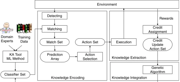
The system architecture is shown in Fig. 1. It is an
implementation version of the general framework of the Wilson’s XCS classifier system. The algorithm of the
XCS-based knowledge integration (XCS-KI) is shown inFig. 2. At
first, the system initializes the classifier set which is originally empty and will be covered by new classifiers automatically. Here, we assume that all knowledge sources are represented by rules, since almost all knowledge derived by knowledge acquisition (KA) tools, or induced by machine learning (ML) methods may easily be translated into or represented by rules. After the next new run of the system, the initialization stage will load the learned classifier rule sets that are ready to be run. In the knowledge encoding phase, the system detects the state of the environment, and encodes each rule among a rule
set into the condition message of a bit-string structure. Then, the system generates the match set from the classifier set which contains the classifiers matched to the condition message. Next, the system produces a prediction array according to the prediction accuracy of matched classifiers, and generates an action set. After that, the system determines the winner action with the highest accuracy, and then executes this winner action within that environment.
In the knowledge integration phase, the system will obtain the rewards from the environment after executing an action, and then goes through the process of credit/rewards allocation to the classifiers in the action set of the previous step. Fig. 1. System architecture of XCS classifier system.
In the knowledge integration phase, the system instantly starts the learning procedure after the process of credit/rewards apportionment for each activity. In the meantime, the system triggers the GA to implement the evolutionary module, i.e. the GA contains selection, crossover, and mutation activities. Finally, it will report the execution performance, and store learning classifier set for the reapplication in the next activity requirements.
3. Knowledge encoding phase
We use a pure binary string to do the genetic coding. A classification rule can be coded since one chromosome consists of several segments. Each segment corresponds to either an attribute in the condition part (the IF part) of the rule or to a class in the conclusion part (the THEN part) of the rule. Each segment consists of a string of genes that takes a binary value of 0 or 1. Each gene corresponds to one linguistic term of the attribute or class. To improve the clarity of the coding, we use a semicolon to separate segments and a colon to separate the IF part and the THEN part.
In this paper we use a well-known example for deciding what sport to play according to ‘Saturday Morning Problem’ to
demonstrate the process of encoding representation (Quinlan,
1986; Yuan & Shaw, 1995). Three sports {Swimming, Volleyball, Weight_lifting} are to be deciding of four attributes {Outlook, Temperature, Humidity, Wind}. The attribute Out-look has three possible values {Sunny, Cloudy, Rain}, attribute Temperature has three possible values {Hot, Mild, Cool}, attribute Humidity has two possible values {Humid, Normal}, and attribute Wind has two possible values {Windy, Not_windy}. Also, assume that a rule set RSq from a knowledge source has the following three rules:
rq1: IF (Outlook is Sunny) and (Temperature is Hot) THEN
Swimming;
rq2: IF (Outlook is Cloudy) and (Wind is Not_windy) THEN Volleyball;
rq3: IF (Outlook is Rain) and (Temperature is Cool) THEN
Weight_lifting;
The intermediate representation of these rules would then be:
rq10 : IF (Outlook is Sunny) and (Temperature is Hot) and
(Humidity is Humid or Normal) and (Wind is Windy or
Not_windy) THEN Swimming;
rq20 : IF (Outlook is Cloudy) and (Temperature is Hot or Mild
or Cool) and (Humidity is Humid or Normal) and (Wind is Not_windy) THEN Volleyball;
rq30 : IF (Outlook is Rain) and (Temperature is Cool) and
(Humidity is Humid or Normal) and (Wind is Windy or Not_windy) THEN Weight_lifting.
The tests with underlines are dummy tests. Also, rqi0 is
logically equivalent to rqi, for iZ1, 2, 3. After translation, the
intermediate representation of each rule is composed of four attribute tests and one class pattern.
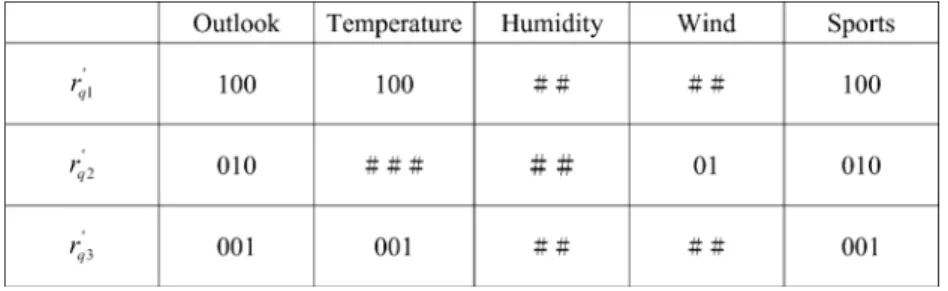
After translation, each intermediate rule in a rule set is ready for being encoded as a bit string. Each attribute test is then encoded into a fixed-length binary string whose length is equal to the number of possible test values. Each bit thus represents a possible value. For example, the set of legal values for attribute Outlook is {Sunny, Cloudy, Rain}, and three bits are used to represent this attribute. Thus, the bit string 110 would represent the test for Outlook being ‘Sunny’ or ‘Cloudy’. With this coding schema, we can also use the all-one string 111 (or simply denoted as #) to represent the wildcard of ‘don’t care’. Continuing the above example, assume each intermediate rule
in RSq is to be encoded as a bit string. We may rewrite rule rq10
as (100; 100; ##; ##: 100). As a result, each intermediate rule in
RSq is encoded into a chromosome as shown inFig. 3. It should
be mentioned that our coding method is suitable to represent multi-value logic with OR relations among terms within each attribute, and the AND relations among attributes. After knowledge encoding, the genetic process chooses bit-string rules for ‘mating’, gradually creating good offspring rules. The offspring rules then undergo iterative ‘evolution’ until an optimal or a nearly optimal set of rules is found.
4. Knowledge extraction phase
In the knowledge extraction phase, genetic operations and credit assignment are applied at the rule level. In our approach, the initial set of bit strings for rules comes from multiple knowledge sources. Each individual within the population is a rule, and is of fixed length. Good rules are then selected for genetic operations to produce better offspring rules. The genetic process runs generation after generation until certain criteria have been met. After evolution, all the rules in a population are then combined to form a resulting rule set.
Fig. 3. Bit-string representation of RSq.
A.-P. Chen, M.-Y. Chen / Expert Systems with Applications 31 (2006) 174–183 176
4.1. Initial population
The GA requires a population of individuals to be initialized and updated during the evolution process. In our approach, the initial set of bit strings for rules comes from multiple knowledge sources. Each individual within the population is a rule, and is of fixed length. If all of rule sets have k rules, then the initial population size is k.
4.2. The strength of a rule
The strength of the fitness of a rule can be measured jointly by its coverage, accuracy, and relative contribution among all
the rules in the population (Liao & Chen, 2001). Let U be the
set of test objects. The coverage of a rule derived rule (ri) is
defined as follows
CgðriÞ Z
jGU
rij
n (1)
where GUri is the set of test objects in U correctly predicted by ri.
The n is the number of objects in U. The coverage Cg(ri) is the relative size of this condition set in the entire object space. Obviously, the larger the coverage, the more general the rule is.
The accuracy of a rule riis evaluated using test objects as
follows: AcðriÞ Z jGU rij jGU rij C jU KG U rij (2) ðU KGU
riÞ is the set of test objects in U wrongly predicted by
ri. The accuracy of the rule is the measure indicating the degree
to which the condition set is the subset of the conclusion set, or the truth that the condition implies the conclusion. Obviously, the higher the accuracy, the better the rule is.
Since an object may be classified by many rules, we want to measure the contribution of each rule in the classification of each object. If an object is classified correctly by only one rule, then this rule has full contribution or credit which equals 1. If
an object is classified correctly by n rules, then these rules should share the contribution, and thus each of them has only 1/n contribution. The contribution of a rule is the sum of its contribution to correctly classify each object. The contribution
of a rule riis defined as follows
CbðiÞ ZX u2U Jðri; uÞ P r0 i2RJðr 0 i; uÞ where
Jðr;uÞZ 1 if u is correctly classified by rule r
0 otherwise
(
(3) The R is the population of all the rules. The u is a test object in U. The contribution measure captures the uniqueness of the rule. A rule with high contribution is generally less overlapping with other rules. Finally, we integrate all the quality measures
into a single fitness function. The fitness of a rule riis defined
by Eq. (4)
FitðriÞ Z ððAcðriÞK1=LÞ CCgðriÞ=LÞCbðriÞ (4)
The L is the number of all possible classes. The Ac(ri) is
subtracted by 1/L represents the accuracy of random guessing among L evenly distributed classes. The reason for making this subtraction is that a useful rule should have more accuracy than random guessing. We use 1/L as the weight for the coverage. When there are more classes, the coverage should have less weight because in this situation accuracy will be more difficult to achieve than coverage. Finally, the sum of the net accuracy and
the weighted coverage is multiplied by the Cb(ri) which
represents the rule’s competitive contribution in the population.
5. Knowledge integration phase
Genetic operators are applied to the population of rule sets for knowledge integration. They could create new rules from existing rules. There are two primitive genetic operators: Table 1
A set of test objects
Case Outlook Temperature Humidity Windy Sports
Sunny Cloudy Rain Hot Mild Cool Humid Normal Windy Not_Windy Swimming Volleyball W-Lifting
1 1 0 0 1 0 0 1 0 0 1 1 0 0 2 1 0 0 1 0 0 0 1 0 1 0 1 0 3 0 1 0 1 0 0 0 1 0 1 1 0 0 4 0 1 0 0 1 0 0 1 0 1 0 1 0 5 0 0 1 1 0 0 0 1 1 0 0 0 1 6 0 1 0 0 0 1 1 0 0 1 0 0 1 7 0 0 1 0 0 1 0 1 0 1 0 0 1 8 0 1 0 0 0 1 0 1 0 1 0 1 0 9 1 0 0 1 0 0 1 0 1 0 1 0 0 10 1 0 0 0 0 1 0 1 1 0 0 0 1 11 1 0 0 1 0 0 1 0 0 1 1 0 0 12 0 1 0 0 1 0 0 1 0 1 0 1 0 13 1 0 0 0 1 0 0 1 1 0 0 0 1 14 0 1 0 0 1 0 0 1 1 0 0 0 1 15 0 0 1 0 0 1 1 0 1 0 0 0 1 16 1 0 0 0 1 0 0 1 0 1 0 1 0
crossover and mutation. The detail operators are described as follows.
The crossover operator exchanges string segments between two parent chromosomes to generate two child chromosomes.
Continuing the above example, assume r1and r2are chosen as
the parents for crossover. Assume the crossover point is set on their first and second segments.
Parent 1: (100; 100; ##; ##; 100) Parent 2: (010; ###; ##; 01; 010) Child 1: (010; ###; ##; ##; 100) Child 2: (100; 100; ##; 01; 010)
The two newly generated offspring rules are then: Child 1: IF (Outlook is Cloudy) then Swimming;
Child 2: IF (Outlook is Sunny) and (Temperature is Hot) and (Wind is Not_windy) THEN Volleyball.
The mutation operator is randomly changes some elements in a selected rule and leads to additional genetic diversity to help the process escape from local-optimum ‘traps’. As an
example, the mutation on the second segment of the r1is shown
as follows: Existing: (100; 100; ##; ##: 100). Mutated: (100; 001; ##; ##: 100) or (100; 010; ##; ##: 100) or (100; 011; ##; ##: 100) or (100; 101; ##; ##: Tabl e 2 The rules in the 28t h g eneration for the Saturda y Morni ng Prob lem Rule Outloo k Temper ature Hum idity Win d y Sports A ccuracy C o verage Fi tness Sunny Cloud y Rain Hot Mild Co ol Hum id N ormal Win d y Not_Win dy Swimmi ng Volle yball W-Lifiting 1* 0 0 1 0 1 1 1 1 1 0 0 0 1 1 0.33 5 0.22 2 1 1 0 0 1 0 0 1 1 1 0 1 0 0.92 0.18 2 0.21 3* 1 1 0 0 1 0 0 1 0 1 0 1 0 1 0.31 2 0.2 4 1 0 0 1 0 0 1 0 1 1 0 0 1 0.74 0.28 4 0.2 5 0 0 1 0 1 1 1 1 1 1 1 0 0 0.96 0.14 2 0.19 6* 1 1 0 1 0 0 1 1 1 1 1 0 0 1 0.32 4 0.18 7 0 0 1 1 1 1 1 0 0 1 0 1 0 0.72 0.24 1 0.17 8 1 0 1 1 1 0 1 1 1 1 1 0 0 0.86 0.16 3 0.16 9 0 1 0 0 0 1 1 1 1 1 0 0 1 0.88 0.23 7 0.15 10 1 1 1 0 1 1 1 0 1 0 1 0 0 0.66 0.13 5 0.14 11 0 1 0 1 0 0 1 0 1 1 0 0 1 0.36 0.44 2 0.14 12 1 0 0 1 0 0 0 1 0 1 0 1 0 0.77 0.21 5 0.13 13 0 1 1 1 1 0 1 0 1 0 0 1 0 0.83 0.27 6 0.12 14 1 1 1 1 1 0 1 0 0 1 0 0 1 0.42 0.13 5 0.11 15 0 1 0 1 1 1 0 1 1 1 1 0 0 0.55 0.11 2 0.1 Table 3
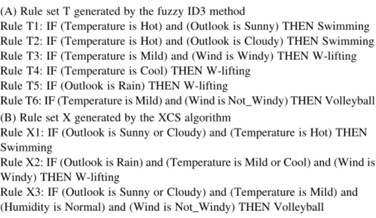
Two sets of rules generated by fuzzy ID3 and XCS algorithm (A) Rule set T generated by the fuzzy ID3 method
Rule T1: IF (Temperature is Hot) and (Outlook is Sunny) THEN Swimming Rule T2: IF (Temperature is Hot) and (Outlook is Cloudy) THEN Swimming Rule T3: IF (Temperature is Mild) and (Wind is Windy) THEN W-lifting Rule T4: IF (Temperature is Cool) THEN W-lifting
Rule T5: IF (Outlook is Rain) THEN W-lifting
Rule T6: IF (Temperature is Mild) and (Wind is Not_Windy) THEN Volleyball (B) Rule set X generated by the XCS algorithm
Rule X1: IF (Outlook is Sunny or Cloudy) and (Temperature is Hot) THEN Swimming
Rule X2: IF (Outlook is Rain) and (Temperature is Mild or Cool) and (Wind is Windy) THEN W-lifting
Rule X3: IF (Outlook is Sunny or Cloudy) and (Temperature is Mild) and (Humidity is Normal) and (Wind is Not_Windy) THEN Volleyball
Fig. 4. A 6-bit multiplexer. A.-P. Chen, M.-Y. Chen / Expert Systems with Applications 31 (2006) 174–183
100) or (100; 110; ##; ##: 100) or (100; 111; ##; ##: 100).
6. Experimental results
Two sample classification problems are used to illustrate the performance of the XCS-KI algorithm. The first is the Saturday Morning Problem, and the second is the Multiplexer Problem.
They each have different structures and a different level of difficulties.
6.1. Saturday Morning Problem
We use the ‘Saturday Morning Problem’ to generate sample data based on existing rules and then test if the hidden rules can be discovered from the sample data by a learning algorithm.
The training data is shown inTable 1.
To apply our algorithm, the population size is fixed to 200. The initial population consists of 16 rules converted from 16 cases, and 184 rules randomly generated. In each generation, 20% of the population is selected for reproduction. The crossover probability is 0.8, and the mutation probability is 0.04. For selecting the replacement candidate, the sub-population size is 20 and initial fitness is 0.01.
The number of rules extracted from the population decreases through generations. The final rule set extracted from the 28th generation consists of three rules. The three rules with * are the rules extracted from the population. They are
listed inTable 2along with 12 other rules that have high fitness
values.Table 2also shows the accuracy and coverage of these
rules. They all have approximately the highest coverage. Finally, among them the rule with the highest fitness value, 0.22, is selected. The final rule set is denoted as set X which
consists of rules X1–X3, and is listed in Table 3(B). For
comparison, another set of rules is generated by using the
Fuzzy Decision Tree Induction method (Yuan & Shaw, 1995)
Fig. 6. The evolution process.
Fig. 5. The classifier format for a 6-bit multiplexer.
Table 4
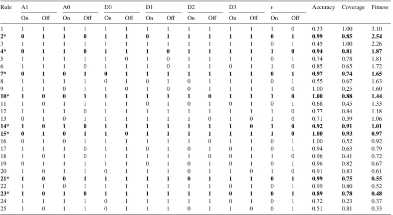
The rules in the 48th generation for the six-bit Multiplexer problem
Rule A1 A0 D0 D1 D2 D3 v Accuracy Coverage Fitness
On Off On Off On Off On Off On Off On Off On Off
1 1 1 1 1 1 1 1 1 1 1 1 1 1 0 0.33 1.00 3.10 2* 0 1 1 0 1 1 0 1 1 1 1 1 0 1 0.99 0.85 2.54 3 1 1 1 1 1 1 1 1 1 1 1 1 0 1 0.45 1.00 2.26 4* 0 1 1 0 1 1 1 0 1 1 1 1 1 0 0.94 0.81 1.87 5 1 1 1 1 1 0 1 0 1 1 1 1 0 1 0.74 0.78 1.81 6 1 1 1 0 1 1 1 0 1 1 0 1 1 0 0.85 0.65 1.72 7* 0 1 0 1 0 1 1 1 1 1 1 1 0 1 0.97 0.74 1.65 8 1 1 1 1 0 1 0 1 0 1 1 1 0 1 0.55 0.67 1.63 9 1 1 0 1 1 0 1 0 0 1 1 1 1 0 1.00 0.25 1.60 10* 1 0 0 1 1 1 1 1 1 0 1 1 1 0 1.00 0.88 1.44 11 1 0 1 1 1 1 0 1 0 1 0 1 0 1 0.68 0.45 1.33 12 1 1 1 0 1 1 1 1 1 1 1 1 1 0 0.77 0.84 1.18 13 0 1 0 1 1 1 1 1 1 0 1 0 1 0 0.71 0.39 1.06 14* 1 0 1 0 1 1 1 1 1 1 1 0 1 0 0.92 0.91 1.01 15* 0 1 0 1 1 0 1 1 1 1 1 1 1 0 1.00 0.93 0.97 16 0 1 0 1 1 1 1 1 1 0 1 1 0 1 1.00 0.52 0.92 17 1 1 1 0 1 1 0 1 0 1 0 1 0 1 0.94 0.63 0.79 18 1 0 1 0 1 1 1 1 1 0 0 1 1 0 0.96 0.41 0.72 19 0 1 1 1 1 1 0 1 0 1 0 1 0 1 0.96 0.82 0.67 20 1 0 1 1 0 1 1 1 0 1 1 0 1 0 0.91 0.83 0.61 21* 1 0 0 1 1 1 1 1 0 1 1 1 0 1 0.99 0.75 0.55 22 1 1 0 1 1 1 1 1 1 1 0 1 0 1 0.99 0.80 0.52 23* 1 0 1 0 1 1 1 1 1 1 0 1 0 1 0.89 0.78 0.48 24 1 1 1 1 0 1 1 1 1 1 0 1 0 1 0.72 0.23 0.37 25 1 0 1 1 0 1 1 1 0 1 1 0 0 1 0.51 0.81 0.33
from the same set of sample data. It is denoted as rule set T
which consists of rules T1–T6 and is listed inTable 3(A).
FromTable 3, it is worth noting that the swimming rule X1 is equivalent to the combination of swimming rules T1 and T2. The weight-lifting rule X2 is a little more specific than the combination of rules T3, T4 and T5. The volleyball rule X3 is
somehow more specific than T6 but is not fully covered by T6. As a result, the rules generated by the XCS algorithm seem to be both more accurate and more general.
6.2. Multiplexer problem
A simple experiment to demonstrate LCS is the 6-bit
multiplexer (Goldberg, 1989). A Boolean 6-bit multiplexer is
composed out of a 6 bit condition part (input) and a 1 bit action
part (output).Fig. 4illustrates the 6-bit multiplexer. The first 2
bits of the input determine the binary address (00,01,10,11) which will select 1 of the 4 data lines. The output is determined
by the value on the current selected dateline.Fig. 5shows the
resulting classifier format for the 6-bit multiplexer. Where msb is the most significant bit and lsb is the least.
Table 5
Format of classifiers
Condition Action
(percentage change of close copq1) lop1 a
(percentage change of ADI copq2) lop2
(percentage change of RSI copq3) lop3
(percentage change of MACD cop4q4)
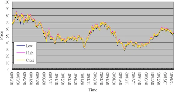
Fig. 7. Stock price from January, 2000 to December, 2003 (by day). (Low: lowest price; High: highest price; Close: close price).
Fig. 8. Technical indicator from January, 2000 to December, 2003 (by day). A.-P. Chen, M.-Y. Chen / Expert Systems with Applications 31 (2006) 174–183 180
With our multi-value logic coding method, each input and output has two values ‘On’ and ‘Off’ and thus can be represented by a string of two bits. We use 10 to represent ‘On’, 01 to represent ‘Off’, and # to represent a wildcard ‘don’t care’. As an example, (0;1;0;0;1;1) has an output of (0) because the input at data line 01 is 0. The format for this example is (0; 1;0;0;1;1:0). It is clear that the input values of the data lines 00, 10 and 11 in this example are not needed to generate the output. Further, the above case can then be represented as (01;10;01; 01;10;10:01). The whole behavior of the 6-bit multiplexer can be summarized in the following eight rules:
Rule 1: (01;01;01;##;##;##:01) Rule 2: (01;01;10;##;##;##:10) Rule 3: (01;10;##;01;##;##:01) Rule 4: (01;10;##;10;##;##:10) Rule 5: (10;01;##;##;01;##:01) Rule 6: (10;01;##;##;10;##:10) Rule 7: (10;10;##;##;##;01:01) Rule 8: (10;10;##;##;##;10:10)
Since there are six binary inputs and one binary output, only a total of 64 different cases can be used for training.
However, with a possible wildcard, we could have 37Z2187
different rules. The total number of different rule sets then is
22187. To determine the optimal set of rules in this huge
search space is not an easy task. We used the XCS-KI algorithm to learn the rules. To apply our algorithm, the population size is fixed to 200. In each generation, 20% of the population is selected for reproduction. The crossover probability is 0.8, and the mutation probability is 0.04. For selecting the replacement candidate, the sub-population size is 20 and the initial fitness is 0.01. The algorithm converges quickly. The optimal set of eight best rules is extracted from the 48th generation. For comparison, another set of eight best rules is generated by using the Fuzzy Decision Tree Induction method from the 68th generation. The number of
rules extracted in each generation is illustrated in Fig. 6.
During the evolution process it gradually decreases, indicating the improvement of the rule set.
The optimal set of eight best rules was extracted from the 48th generation, which 17 other rules that have the highest
fitness values shown in Table 4. The eight rules with * are
the best rules extracted from the population. Notice that the two rules with the highest fitness values are the most general rules.
7. Empirical study and performance evaluation 7.1. Experiment design
The TSMC (Taiwan Semiconductor Manufacturing Com-pany) stock listed in the Taiwan Stock Exchange is selected to Table 6
Experiment performance
Algorithm Experiment Profit
(%)
Accuracy (%) XCS-KI A: 20 Learning sub-steps 74.12 67.54
B: 50 Learning sub-steps 96.48 78.67 C: 80 Learning sub-steps 87.63 77.25
ID3 A: 20 Learning sub-steps 52.74 54.56
B: 50 Learning sub-steps 58.67 55.33 C: 80 Learning sub-steps 54.52 55.19 Fuzzy ID3 A: 20 Learning sub-steps 52.89 57.11 B: 50 Learning sub-steps 67.42 61.46 C: 80 Learning sub-steps 69.13 72.28 Neural network A: 20 Learning Sub-steps 66.41 68.79 B: 50 Learning Sub-steps 79.65 73.65 C: 80 Learning Sub-steps 78.73 71.55 Genetic algorithm A: 20 Learning sub-steps 61.41 68.79 B: 50 Learning sub-steps 67.65 73.65 C: 80 Learning sub-steps 71.73 71.55
verify the capability of our XCS-KI algorithm. Founded in 1987, TSMC is the world’s largest dedicated semiconductor foundry. As the founder and leader of this industry, manufacturing capacity of TSMC is currently about 4.3 million wafers, while its revenues represent some 60% of the global foundry market. In this experiment, the condition part of a trading rule (classifier) consists of three comparisons con-nected by two logical operators. Each comparison uses one of the following four technical indicators:
† percentage change of close,
† percentage change of ADI (Average Directional Index), † percentage change of RSI (Relative Strength Index), and † percentage change of MACD (Moving Average
Conver-gence & DiverConver-gence).
The action part of a trading classifier is long, short, or none representing corresponding action for the next trading day. The format of classifiers in the model is shown in
Table 5, where cop’s stand for the comparison operators (OZ, !), lop’s stand for the logical operators (AND, OR), q’s stand for the thresholds and a stands for the action (long, short, none).
The trading period of our experiment is from January 4, 2000 to December 29, 2003, with 1009 trading days. We test three heuristically decided learning sub-steps.
Each setting runs three times to get its average
performance. Fig. 7 shows the basic stock price
information about TSMC. Furthermore, we calculate the advance technical indicator to analyze the TSMC stock
price in Fig. 8.
Fig. 10. Equity curve of 50 instant learning sub-steps.
Fig. 11. Equity curve of 80 instant learning sub-steps.
A.-P. Chen, M.-Y. Chen / Expert Systems with Applications 31 (2006) 174–183 182
7.2. Performance evaluation
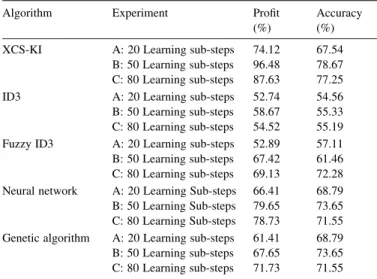
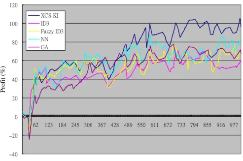
In this experiment, profit and accuracy of the proposed approach is compared to that of the other classification methods (decision tree, fuzzy decision tree, neural network, and genetic algorithm). The detail experiment performances
are summarized in Table 6. The profit is the accumulated
rate of return for each trading day. Figs. 9–11 show the
equity curves of 20, 50, and 80 instant learning sub-steps, respectively. The results of these experiments can be summarized as follows.
1. The average profit of experiment B of 50 instant learning sub-steps is 96.48% is better than other machine learning algorithms. It shows that the model really could get a remarkable profit in the security trading problem. 2. The correct rate of experiment B is 78.67%, and all the
correct rates of these three experiments are better than the correct rate of average random trading action strategy (33.33%), and other machine learning algorithms. There-fore, it proves the proposed approach is more accurate than other machine learning algorithm.
3. The 50 instant learning sub-steps experiment is the best one of these three experiments. It seems that too small instant learning sub-steps could not learn the experience. Besides, it proves the proposed approach has high performance than other machine learning algorithm.
8. Conclusion
In this paper, we have shown how the knowledge encoding, extraction, and integration methodology can be effectively represented and addressed by the proposed XCS-KI algorithm. The main contributions are: (1) it needs no human experts’ intervention in the knowledge integration process; (2) it is capable of generating classification rules that can be applied when the number of rule sets to be integrated increases; (3) it uses three criteria (accuracy, coverage, and fitness) to apply the knowledge extraction process which is very effective in selecting an optimal set of rules from a large population. The experiments prove that the rule sets derived by the proposed approach are more accurate than other machine learning algorithm.
References
Baral, C., Kraus, S., & Minker, J. (1991). Combining multiple knowledge bases. IEEE Transactions on Knowledge and Data Engineering, 3(2), 208– 220.
Boose, J. H., & Bardshaw, J. M. (1987). Expertise transfer and complex problems: Using AQUINAS as a knowledge-acquisition workbench for knowledge-based systems. International Journal of Man–Machine Studies, 26, 3–28.
Giarratano, J., & Riley, G. (1998). Expert systems—principle and programming (3rd ed.). Boston, MA: PWS Publishing Company.
Goldberg, D. E. (1989). Genetic algorithms in search, optimization, and machine learning. Reading, MA: Addison-Wesley.
Hashemi, R. R., Blanc, L. A., Rucks, C. T., & Rajaratnam, A. (1998). A hybrid intelligent system for predicting bank holding structures. European Journal of Operational Research, 109, 390–402.
Holland, J. H. (1975). Adaptation in natural and artificial systems. Ann Arbor, MI: University Press of Michigan.
Holland, J. H., & Reitman, J. S. (1978). Cognitive systems based on adaptive algorithms. In D. A. Waterman, & F. Hayes-Roth (Eds.), Pattern directed interference systems (pp. 313–329). New York: Academic Press. Holmes, J. H. (1996). Evolution-assisted discovery of sentinel features in
epidemiologic surveillance. PhD thesis, Drexel University, Philadelphia, PA. Kovalerchuk, B., & Vityaev, E. (2000). Data mining in finance. Dordrecht:
Kluwer.
Liao, P. Y., & Chen, J. S. (2001). Dynamic trading strategy learning model using learning classifier systems. Proceedings of the 2001 Congress on Evolutionary Computation (pp. 783–789).
McIvor, R. T., McCloskey, A. G., Humphreys, P. K., & Maguire, L. P. (2004). Using a fuzzy approach to support financial analysis in the corporate acquisition process. Expert Systems with Applications, 27, 533–547. Oh, K. J., Kim, T. Y., & Min, S. (2005). Using genetic algorithm to support
portfolio optimization for index fund management. Expert Systems with Applications, 28, 371–379.
Quinlan, J. (1986). Induction of decision tree. Machine Learning, 1, 81–106.
Shin, H. W., & Sohn, S. Y. (2003). Combining both ensemble and dynamic classifier selection schemes for prediction of mobile internet subscribers. Expert Systems with Applications, 25, 63–68.
Stolzmann, W. (2000). An introduction to anticipatory classifier systems. Lecture notes in artificial intelligence, 1813, 175–194.
Trippi, R. R., & Desieno, D. (1992). Trading equity index futures with a neural network. Journal of Portfolio Management, Fall , 27–33.
Wang, Y. F. (2003). Mining stock price using fuzzy rough set system. Expert Systems with Applications, 24, 13–23.
Wilson, S. W. (1996). Rule strength based on accuracy. Evolutionary Computation, 3(2), 143–175.
Yuan, Y., & Shaw, M. J. (1995). Induction of fuzzy decision trees. Fuzzy Sets and Systems, 69, 125–139.
Yuan, Y., & Zhuang, H. (1996). A genetic algorithm for generating fuzzy classification rules. Fuzzy Sets and Systems, 84, 1–19.