藉變強度耦合、適應控制及部份區域穩定理論之渾沌系統同步與非同步性

國立交通大學

機械工程學系

博士論文

藉變強度耦合、適應控制及部份區域穩定理論

之渾沌系統同步與非同步

Unsynchronizability and Synchronization of Chaotic System

by Variable Strength Coupling, by Adaptive Control

and by Partial Stability Theory

研 究 生：鄭普建

指導教授：戈正銘 教授

中華民國九十六年十二月

藉變強度耦合、適應控制及部份區域穩定理論

之渾沌系統同步與非同步

Unsynchronizability and Synchronization of Chaotic System

by Variable Strength Coupling, by Adaptive Control

and by Partial Stability Theory

研 究 生：鄭普建 Student：Pu-Chien Tsen

指導教授：戈正銘 Advisor：Zheng-Ming Ge

國 立 交 通 大 學

機 械 工 程 學 系

博 士 論 文

Submitted to Department of Mechanical Engineering College of Engineering

National Chiao Tung University In Partial Fulfillment of the Requirements

for the Degree of Doctor of Philosophy

in

Mechanical Engineering December 2007

Hsinchu, Taiwan, Republic of China

藉變強度耦合、適應控制及部份區域穩定理論

之渾沌系統同步與非同步

國立交通大學機械工程學系

摘要

Unsynchronizability and Synchronization of Chaotic System

by Variable Strength Coupling, by Adaptive Control

and by Partial Stability Theory

Student：Pu-Chien Tsen Advisor：Zheng-Ming Ge Department of Mechanical Engineering

National Chiao Tung University

Abstract

This thesis consists of three parts：(1) two theorems of unsynchronizability and synchronization for coupled chaotic systems and two theorems of generalized unsynchronization for coupled chaotic systems. (2) chaos synchronization by variable strength linear coupling and Lyapunov function derivative in series form and adaptive chaos synchronization by variable strength linear coupling. (3) chaos generalized synchronization and chaos control by partial region stability theory.

CONTENTS

摘要………

i

ABSTRACT………...………... ii

CONTENTS………...……….………….iii

LIST OF FIGURES………..………... v

Chapter 1 Introduction ………..…………..………...….… 1

Chapter 2 The Theorems of Unsynchronizability and Synchron

-ization for Coupled Chaotic Systems……… 3

2.1 Preliminary………..………...……… 3

2.2 Two Theorems of Unsynchronizability………....…… 3

2.3 Simulated Examples... 10

2.4 Summary………..……….…... 12

Chapter 3 Two Theorems of Generalized Unsynchronization for

Coupled Chaotic Systems……… 20

3.1 Preliminary………..………...………..……… 20

3.2 Two Theorems of Generalized Unsynchronizability………. 20

3.3 Simulated Examples……… 27

3.4 Summary………..……….…….. 28

Chapter 4 Chaos Synchronization by Variable Strength Linear

Coupling and Lyapunov Function Derivative in Series

Form………..….…… 36

4.1 Preliminary………...……….……. 36

4.2 Synchronization strategy by variable strength linear coupling and Lyapunov function derivative in series form……… 36

4.3 Numerical results for typical chaotic systems………..……… 39

4.4 Summary……….……….… 43

Chapter 5 Adaptive Chaos Synchronization by Variable Strength

Linear Coupling………. 49

5.2 Adaptive Chaos Synchronization Strategy by Variable Strength Linear

Coupling………...………. 49

5.3 Numerical results for typical chaotic systems………..… 51

5.4 Summary……….……….… 54

Chapter 6 Chaos Generalized Synchronization by Partial Region

Stability Theory………..……... 60

6.1 Preliminary………...…………..…….…. 60

6.2 Chaos Generalized Synchronization Strategy by Partial Region Stability Theory………...………….… 60

6.3 Numerical Simulations……… 67

6.4 Summary……….……….……… 71

Chapter 7 Chaos Control by Partial Region Stability Theory..….. 78

7.1 Preliminary………...…….………... 78

7.2 Chaos Control Scheme……….78

7.3 Numerical Simulations………….………..………. 79

7.4 Summary……….………. 82

Chapter 8 Conclusions……… 88

REFERENCES………..…… 90

List of Figures

Fig. 2.1 D region for n=2.………..……….………….……… 13 Fig. 2.2 D region for n=2.……….……….……….………. 13 Fig. 2.3 Chaotic attractor for Chen system (2.25a), with a=35,b= and 3 c=28, initial condition (0.5,1,5)……….………...…… 14 Fig. 2.4 Lyapunov exponents for Chen system (2.25a), with b=3 and c=28, initial condition (0.5,1,5).………..……… 14 Fig. 2.5 Chaotic attractor for chaotic system (2.25b), with a=35,b= and 3

28

c= , initial condition (30,20,18).………..……….……15 Fig. 2.6 Lyapunov exponents for chaotic system (2.25b) , with b=3 and c=28, initial condition (30,20,18).………...…. 15 Fig. 2.7 State errors versus time for unidirectional coupled systems (2.25), with

35

a= , b=3 and c=28, initial conditions (0.5,1,5), (30,20,18)….… 16 Fig. 2.8 State errors versus time for unidirectional coupled systems (2.25) , with

35, 3

a= b= and c=28, initial conditions (0.5,1,5), (30,20,18).……... 16 Fig. 2.9 Lyapunov exponents for Rössler system (2.26a), with b=0.2 and

5.7

c= , initial condition (20,10,25)………..……… 17 Fig. 2.10 Lyapunov exponents for chaotic system (2.26b), with b=0.2 and

5.7

c= , initial condition (2.5,2,2.5).………..………... 17 Fig. 2.11 State errors versus time for unidirectional coupled systems (2.26), with

0.2, 0.2

a= b= and c=5.7, initial conditions (20,10,25), (2.5,2,2.5)… 18 Fig. 2.12 Lyapunov exponents for Duffing system, with α β ω= = = and 1

0.15

δ = , initial condition (2,2)………. 18 Fig. 2.13 Lyapunov exponents for chaotic system (2.27b), with α β ω= = = and 1

0.15

δ = , initial condition (0.1,0).…………..……….……… 19 Fig. 2.14 State errors versus time for unidirectional coupled systems (2.27), with

0.15

δ = , α β ω= = = and 1 a=3, initial conditions (2,2), (0.1,0)….. 19 Fig. 3-1 D region for n=2.……… 29 Fig. 3-2 D region for n=2.………..………. 29 Fig. 3.3 Chaotic attractor for Chen system (3.24a), with a=35,b= and 3 c=28, initial condition (0.5,1,5).………..… 30

Fig. 3.4 Lyapunov exponents for Chen system (3.24a), with b=3 and c=28, initial condition (0.5,1,5).………..………... 30 Fig. 3.5 Chaotic attractor for chaotic system (3.24b), with a=35,b= and 3

28

c= , initial condition (30,20,18).……….……… 31 Fig. 3.6 Lyapunov exponents for chaotic system (3.24b), with b=3 and c=28, initial condition (30,20,18).………..……… 31 Fig. 3.7 State errors versus time for unidirectional coupled systems (3.24), with

35, 3

a= b= and c=28, initial conditions (0.5,1,5), (30,20,18).…..… 32 Fig. 3.8 Errors versus time for unidirectional coupled systems (3.24), with a=35,

3

b= and c=28, initial conditions (0.5,1,5), (30,20,18).………... 32 Fig. 3.9 Errors versus time for unidirectional coupled systems (3.24), with

35, 3

a= b= and c=28, initial conditions (0.5,1,5), (30,20,18).…….. 33 Fig. 3.10 Lyapunov exponents for Rössler system (3.25a), with b=0.2 and

5.7

c= , initial condition (20,10,25)………..……….... 33 Fig. 3.11 Lyapunov exponent for chaotic system (3.25b), with b=0.2 and c=5.7, initial condition (2.5,2,2.5)………..…. 34 Fig. 3.12 State errors versus time for unidirectional coupled systems (3.25) , with

0.2, 0.2

a= b= and c=5.7, initial conditions (20,10,25), (2.5,2,2.5)... 34 Fig. 3.13 Errors versus time for unidirectional coupled systems (3.25), with

0.2, 0.2

a= b= and c=5.7, initial conditions (20,10,25), (2.5,2,2.5)… 35 Fig. 3.14 Errors versus time for unidirectional coupled systems (3.25), with

0.2, 0.2

a= b= and c=5.7, initial conditions (20,10,25), (2.5,2,2.5)… 35 Fig. 4.1 Chaotic phase portraits for Rössler system.………... 45 Fig. 4.2 Time histories of errors for two Rössler systems.……….……… 45 Fig. 4.3 Chaotic phase portraits for Hyper-Rössler system.……… 46 Fig. 4.4 Time histories of errors for two synchronized Hyper-Rössler systems…. 46 Fig. 4.5 Chaotic phase portrait for Duffing system.……….…….. 47 Fig. 4.6 Time histories of errors for two synchronized Duffing systems…..……. 47 Fig. 4.7 Chaotic phase portraits for Lorenz system.……….……….. 48 Fig. 4.8 Time histories of errors for two synchronized Lorenz systems.……..….. 48 Fig. 5.1 Time histories of errors for Lorenz system.………...……… 57 Fig. 5.2 Time histories of estimated parameters for Lorenz system.…………...… 57

Fig. 5.4 Time histories of estimated parameters for Duffing system.……….…… 58

Fig. 5.5 Time histories of errors for Rössler system.………..…… 59

Fig. 5.6 Time histories of estimated parameters for Rössler system…………..… 59

Fig. 6.1 Partial region Ω .……… 72

Fig. 6.2 Phase portrait of error dynamics for Case I………..… 72

Fig. 6.3 Time histories of errors for Case I.……… 73

Fig. 6.4 Time histories of x1, x2, x3, y1, y2, y3 for Case I.………... 73

Fig. 6.5 Phase portrait of error dynamics for Case II.……….... 74

Fig. 6.6 Time histories of errors for Case II.………... 74

Fig. 6.7 Time histories of x_i− +y_i 100 and −Fsinωt for Case II.……… 75

Fig. 6.8 Phase portrait of error dynamics for Case III.………... 75

Fig. 6.9 Time histories of errors for Case III.………... 76

Fig. 6.10 Phase portrait of error dymanics for Case IV………..….. 76

Fig. 6.11 Time histories of errors for Case IV……….. 77

Fig. 6.12 Time histories of x y− +100 and −z for Case IV……….... 77

Fig. 7.1 Chaotic phase portrait for Lorenz system in the first quadrant………… 83

Fig. 7.2 Phase portrait of error dynamics for Case I………...… 83

Fig. 7.3 Time histories of x1, x2, x3 for Case I.……….. 84

Fig. 7.4 Phase portrait of error dynamics for Case II... 84

Fig. 7.5 Time histories of errors for Case II.………... 85

Fig. 7.6 Time histories of x1, x2, x3 for Case II……….… 85

Fig. 7.7 Phase portrait of error dynamics for Case III………. 86

Fig. 7.8 Time histories of errors for Case III.……….. 86

Chapter 1

Introduction

In recent years, synchronization in chaotic dynamic system is a very interesting problem and has been widely studied [1-8]. Synchronization means that the state variables of a response system approach eventually to that of a drive system. There are many control techniques to synchronize chaotic systems, such as linear error feedback control, adaptive control, active control [9-19]. Besides, generalized synchronization also has been investigated in various fields. Generalized synchronization means that there is a functional relation between the states of driving system and response system.

Recently, the synchronization criteria of unidirectional coupled chaotic systems by partial stability theory are presented [20]. In Chapter 2 of this thesis, we propose two theorems which give the criteria of unsynchronizability for two different chaotic dynamic systems. Chen system, Rössler system and Duffing system with corresponding new chaotic systems proposed are presented as simulated examples for these two theorems [21-22].

In Chapter 3, we propose two theorems which give the criteria of generalized unsynchronization for two different chaotic dynamic systems with whatever large strength of linear coupling. Chen system and Rössler system with corresponding new chaotic systems proposed are presented as simulated examples for these two theorem . In Chapter 4, a new general strategy to achieve chaos synchronization by variable strength linear coupling without another active control is proposed, in which Lyapunov function derivative in series form is first used. This method can give either local synchronization which is usually good enough or global synchronization which

is usually an unnecessary high demand [23-25]. Lorenz system, Duffing system, Rössler system and Hyper-Rössler system are presented as simulated examples.

There are many control techniques to synchronize chaotic systems, but most of them are based on the exact knowledge of the system structure and parameters. In practice, some or all of the system parameters are uncertain, adaptive control method in used. In Chapter 5, we propose a general strategy to achieve adaptive chaos synchronization by variable strength linear coupling solely without using another active control which is usually rather complex. Furthermore, Lyapunov function derivative in series form is first used, which is easier to be obtained than the traditional negative sum of the square of error variables. Lorenz system, Duffing system and Rössler system are presented as simulation examples.

In Chapter 6, a new chaos generalized synchronization strategy by partial region stability theory is proposed [26-27]. By using the theory of stability on partial region the Lyapunov function is a simple linear homogeneous function of states and the controllers are simpler and have less simulation error because they are in lower order than that of traditional controllers where the stability of solutions on the whole neighborhood region of the origin is demanded. Lorenz system and Rössler system are used as simulated examples.

In Chapter 7, a new scheme to achieve chaos control by partial region stability theory is proposed [28]. By using the theory of stability on partial region the Lyapunov function is a simple linear homogeneous function of states and the controllers are simpler and have less simulation error.

Chapter 2

The Theorems of Unsynchronizability and Synchronization

for Coupled Chaotic Systems

2.1 Preliminary

Synchronization in chaotic dynamic system is a very interesting problem and has been widely studied in these years. Synchronization means that the state variables of a response system approach eventually to that of a drive system. There are many control techniques to synchronize chaotic systems, such as linear error feedback control, adaptive control, active control. Recently, the synchronization criteria of unidirectional coupled chaotic systems by partial stability theory are presented. In this Chapter, we propose two theorems which give the criteria of unsynchronizability for two different chaotic dynamic systems. Chen system and a new chaotic system which we proposed are presented as simulated examples for the first theorem. Rössler system and Duffing system with two corresponding new chaotic systems proposed are presented as simulated examples for the second theorem.

2.2 Two Theorems of Unsynchronizability

Consider the following nonautomonous systems

1 = ( ,t 1) x f x (2.1) where _x1∈_{R ,} n 1 : n n + Ω ⊂ × →

f R R R . Eq. (2.1) is considered as a master system. A

slave system is given by

2 = ( ,t 2) x g x (2.2) where _x2∈_{R ,} n 2 : n n + Ω ⊂ × →

and f( , )t 0 =g 0( , )t =0 . Ω , ₁ Ω are domains containing the origin. Assume that ₂

the solutions of Eqs. (2.1) and (2.2) are bounded then they must exist for infinite time. That is, for given ( ,t₀ x₁₀, x₂₀)∈ Ω₁∩Ω₂ the solutions x₁( , ,t t₀ x₁₀, x₂₀) ,

2( , ,t t0 10, 20)

x x x of Eqs. (2.1) and (2.2) exist for t ≥ . If t₀ f( x) g( x) , system t, = t,

(2.1) and (2.2) are two identical systems. When f( x) g( x)t, ≠ t, , they are two different systems.

Now we consider the following unidirectional nonautonomous coupled system

1 1 2 2 1 2 ( , ) ( , ) ( , , ) t t t = = + x f x x g x U x x (2.3)

where U( ,t x x₁, )₂ is a coupled term. In order to discuss the synchronization of x₁ and x₂, define e=x₂ −x₁ as the state error. Error equation can be written as

1 1 1 1

( ,t ) ( ,t ) ( ,t , )

= + − + +

e g e x f x U x e x (2.4)

Now the first theorem will be given for a special case of Eqs. (2.3). Consider unidirectional coupled nonautonomous systems as

1 1 2 2 1 2 ( , ) ( , ) ( ) t t = = + − x f x x g x Γ x _{x (2.5)}

where f and g satisfy Lipschitz condition, and the Lipschitz constant of g is L .

n n

M _×

∈

Γ is a constant diagonal matrix with positive entries, represents the strength of the linear coupling term x₁−x₂. Since e=x₂ −x₁, the error dynamic equation can be obtained as

1 1

( ,t ( ))t ( , ( ))t t

= + − −

e g e x f x Γe (2.6)

which is a nonautonomous system of differential equations for state e and has a null solution e=0,x₁ =0. Now we give a definition of unsynchronizability:

Definition If no positive constant C can be found such that e→0 as t→ ∞ for all

0

( )t <C

e , systems (2.5) are unsynchronizable.

however large coupling strength Γ with positive entries, if f ti( , )x1 ≤g ti( , )x1

(i= …1, , )n in Ω1∩Ω2 , and f( , )t x1 −g x( , )t 1 >0 except at origin, for any

solution x₁( )t .

Proof. Choose a Lyapunov function V( )e =e e1 2 en which is positive in quadrant

1 0, 2 0, , n 0

e > e > e > , then V along any state trajectory of system (2.6) [25]

becomes: 2 3 1 1 3 2 1 2 1 2 3 1 1 1 1 1 1 1 3 2 1 2 1 2 2 1 2 1 1 1 2 3 1 1 1 1 1 1 1 1 1 1 [ ( , ) ( , ) ] [ ( , ) ( , ) ] [ ( , ) ( , ) ] [ ( , ) ( , ) ( , ) ( , ) ] n n n n n n n n n n n n V e e e e e e e e e e e e e e e g t f t e e e e g t f t e e e e g t f t e e e e g t g t g t f t e e − − = + + + = + − − Γ + + − − Γ + + − − Γ = + − + − − Γ + + e x x e x x e x x e x x x x _{1 2 1} 1 1 1 1 [ ( , ) ( , ) ( , ) ( , ) ] n n n n n n n e e g t g t g t f t e − + − + − − Γ e x x x x When e₁>0,e₂ >0, ,en > , we have 0 2 3 1 1 1 1 1 1 1 1 1 1 1 2 1 1 1 1 1 2 3 1 1 1 1 1 1 [ ( , ) ( , ) ( , ) ( , ) ] [ ( , ) ( , ) ( , ) ( , ) ] [ ( , ) ( , ) ] n n n n n n n n n V e e e g t g t g t f t e e e e g t g t g t f t e e e e L g t f t e − ≤ + − + − − Γ + + + − + − − Γ ≤ + − − Γ + e x x x x e x x x x e x x (2.7) where g t₁( ,e x+ ₁)−g t₁( , )x₁ ≤L e follows the Lipschitz condition. When e 1,

the terms of lower degree of error components e e_{2 3} e g tn[ ( , )₁ x₁ − f t₁( , )]x₁ ,

1 3 n[ ( , )2 1 2( , )]1

e e e g t x − f t x , can be neglected when the sign of V is considered,

then

2 3 n[ 1 1] 1 3 n[ 2 2]

V ≤e e e L e − Γe +e e e L e − Γ e + (2.8)

For sufficient large Γ , V can be negative in the quadrant _i e₁> , 0 e₂ > , 0 ,

0

n

e > . So the state point tends to decrease e( )t with time when e₀ is sufficiently large. When e 1 , the proof is as follows. Now when

1 0, 2 0, , n 0 e > e > e > , V is expressed as 2 3 1 1 1 1 1 1 1 1 1 1 2 3 1 1 1 1 1 1 [ ( , ) ( , ) ( , ) ( , ) ] [ ( , ) ( , ) ] n n V e e e g t g t g t f t e e e e L g t f t e ≥ − + − + − − Γ + ≥ − + − − Γ + e x x x x e x x (2.9)

When e 1, the terms of higher degree e e_{2 3} e_n[−L e − Γ_{1 1}e], can be neglected when the sign of V is considered, then

2 3 n[ ( , )1 1 1( , )]1 1 3 n[ ( , )2 1 2( , )]1

V ≥e e e g t x − f t x +e e e g t x − f t x + (2.10)

By the condition f( , )t x₁ −g x( , )t ₁ >0, f t_i( , )x₁ =g t_i( , )x₁ (i=1, , )n do not occur

simultaneously except at the origin x₁ =0. Therefore the right-hand side of above inequality is positive, i.e. V is positive in region D of Fig. 2.1, which is the quadrant

1 0

e > , e₂ > , 0 , 0e_n > of the neighborhood of the origin.

Choose r>0 such that for the ball B_r = ∈{e Rn e ≤r}, we have

{ _r ( ) 0}

D= ∈e B V e > (2.11)

of which the boundary is the surface V( ) 0e = and the sphere e =r . Since ( ) 0

V 0 = , the origin lies on the boundary of D inside B . The point _r e is in the ₀

interior of D and V( )e₀ = >b 0. Now we prove that the trajectory e( )t started at

0

(0)=

e e must leave the set D, i.e. the trajectory must leave the neighborhood of

origin, e cannot approach zero. To see this point, notice that as long as ( )e t is

inside D, ( ( ))V e t ≥b since ( ) 0V e > in D. Let

min{ ( )V D and V( ) b}

β = e e∈ e ≥ (2.12)

which exists since the continuous function ( )V e has a minimum over the compact

set {e∈D and V( )e ≥b}= ∈{e B and V_r, ( )e ≥b} [29]. Then, β > and 0

0 _{0 0}

( ( )) ( ) t ( ( )) t

V e t =V e +

∫

∫

on D. Now, ( )e t cannot leave D through the surface ( ) 0V e = since ( ( ))V e t ≥b.

Hence, it must leave D through the sphere e =r, i.e. it must leave the neighborhood

of the origin, e can never approach zero. Two different dynamic systems in Eq.(2.5) are unsynchronizable for however large Γ .

Theorem 2.2 Two different dynamic systems in Eq. (2.5) is unsynchronizable for

however large coupling strength Γ , if f ti( , )x₁ ≥g ti( , )x₁ (i= …1, , )n in Ω1∩Ω2,

and f t( , )x₁ −g t( , )x₁ >0 except at origin, for any solution x₁( )t .

Proof. Choose a Lyapunov function V( )e =e e_{1 2} en , then V along any state

trajectory of system (2.6) becomes:

Case 1. When n is odd, V e is negative in quadrant ( ) e₁<0,e₂<0, e_n < . 0

2 3 1 1 3 2 1 2 1 2 3 1 1 1 1 1 1 1 1 1 1 1 2 1 1 1 1 1 [ ( , ) ( , ) ( , ) ( , ) ] [ ( , ) ( , ) ( , ) ( , ) ] n n n n n n n n n n n n V e e e e e e e e e e e e e e e g t g t g t f t e e e e g t g t g t f t e − − = + + + = + − + − − Γ + + + − + − − Γ e x x x x e x x x x When e₁<0,e₂<0, e_n < , we have 0 2 3 1 1 1 1 1 1 1 1 1 1 1 2 1 1 1 1 1 2 3 1 1 1 1 1 1 [ ( , ) ( , ) ( , ) ( , ) ] [ ( , ) ( , ) ( , ) ( , ) ] [ ( , ) ( , ) ] n n n n n n n n n V e e e g t g t g t f t e e e e g t g t g t f t e e e e L g t f t e − ≥ − + − + − − Γ + + − + − + − − Γ ≥ − + − − Γ + e x x x x e x x x x e x x (2.14) where g t₁( ,e x+ ₁)−g t₁( , )x₁ ≤L e follows the Lipschitz condition. When e 1,

the terms of lower degree of error components e e_{2 3} e g t_n[ ( , )₁ x₁ − f t₁( , )]x₁ ,

1 3 n[ ( , )2 1 2( , )]1

e e e g t x − f t x , can be neglected when the sign of V is considered,

then 2 3 1 1 1 3 2 2 2 3 1 1 1 3 2 2 [ ] [ ] [ ] [ ] n n n n V e e e L e e e e L e e e e L e e e e L e ≥ − − Γ + − − Γ + = − + Γ − + Γ + e e e e (2.15)

For sufficient large Γ , V can be positive in the quadrant _i e₁ < , 0 e₂< , 0 ,

0

n

e < . So the state point tends to decrease e( )t with time when e₀ is sufficiently large. When e 1, the proof is as follows. Now when e₁< 0, e₂ < 0,

0 n e < , V is expressed as 2 3 1 1 1 1 1 1 1 1 1 1 2 3 1 1 1 1 1 1 [ ( , ) ( , ) ( , ) ( , ) ] [ ( , ) ( , ) ] n n V e e e g t g t g t f t e e e e L g t f t e ≤ + − + − − Γ + ≤ + − − Γ + e x x x x e x x (2.16)

When e 1, the terms of higher degree e e_{2 3} e L_n[ e − Γ_{1 1}e], can be neglected when the sign of V is considered, then

2 3 n[ ( , )1 1 1( , )]1 1 3 n[ ( , )2 1 2( , )]1

V ≤e e e g t x − f t x +e e e g t x − f t x + (2.17)

By the condition f( , )t x₁ −g x( , )t ₁ >0, f t_i( , )x₁ =g t_i( , )x₁ (i=1, , )n do not occur

simultaneously except at x₁=0 . Therefore the right-hand side of above inequality is

negative, i.e. V is negative in region D of Fig. 2.2, which is the quadrant e₁< , 0

2 0

e < , , 0e_n < of the neighborhood of the origin.

Choose r>0 such that for the ball B_r = ∈{e Rn e ≤r}, we have

{ r ( ) 0}

D= ∈e B V e < (2.18)

By the similar reasoning as that in the latter part of the proof for Theorem1, we can prove that the state trajectory started from D must leave the neighborhood of the origin, e can never approach zero. Two different dynamic systems in Eq. (2.5) are unsynchronizable for however large Γ .

2 3 1 1 3 2 1 2 1 2 3 1 1 1 1 1 1 1 1 1 1 1 2 1 1 1 1 1 [ ( , ) ( , ) ( , ) ( , ) ] [ ( , ) ( , ) ( , ) ( , ) ] n n n n n n n n n n n n V e e e e e e e e e e e e e e e g t g t g t f t e e e e g t g t g t f t e − − = + + + = + − + − − Γ + + + − + − − Γ e x x x x e x x x x When e₁<0,e₂<0, en < , we have 0 2 3 1 1 1 1 1 1 1 1 1 1 1 2 1 1 1 1 1 2 3 1 1 1 1 1 1 [ ( , ) ( , ) ( , ) ( , ) ] [ ( , ) ( , ) ( , ) ( , ) ] [ ( , ) ( , ) ] n n n n n n n n n V e e e g t g t g t f t e e e e g t g t g t f t e e e e L g t f t e − ≤ − + − + − − Γ + + − + − + − − Γ ≤ − + − − Γ + e x x x x e x x x x e x x (2.21) where g t₁( ,e x+ ₁)−g t₁( , )x₁ ≤L e follows the Lipschitz condition. When e 1,

the terms of lower degree of error components e e_{2 3} e g tn[ ( , )₁ x₁ − f t₁( , )]x₁ ,

1 3 n[ ( , )2 1 2( , )]1

e e e g t x − f t x , can be neglected when the sign of V is considered,

then 2 3 1 1 1 3 2 2 2 3 1 1 1 3 2 2 [ ] [ ] [ ] [ ] n n n n V e e e L e e e e L e e e e L e e e e L e ≤ − − Γ + − − Γ + = − + Γ − + Γ + e e e e (2.22)

For sufficient large Γ , V can be negative in the quadrant _i e₁< , 0 e₂ < , 0 ,

0

n

e < . So the state point tends to decrease e( )t with time when e₀ is sufficiently large. When e 1, the proof is as follows. Now when e₁< , 0 e₂ < , 0

, 0e_n < , V is expressed as 2 3 1 1 1 1 1 1 1 1 1 1 2 3 1 1 1 1 1 1 [ ( , ) ( , ) ( , ) ( , ) ] [ ( , ) ( , ) ] n n V e e e g t g t g t f t e e e e L g t f t e ≥ + − + − − Γ + ≥ + − − Γ + e x x x x e x x (2.23)

When e 1, the terms of higher degree e e_{2 3} e L_n[ e − Γ_{1 1}e], can be neglected when the sign of V is considered, then

2 3 n[ ( , )1 1 1( , )]1 1 3 n[ ( , )2 1 2( , )]1

By the condition f( , )t x₁ −g x( , )t ₁ >0, f t_i( , )x₁ =g t_i( , )x₁ (i=1, , )n do not occur

simultaneously except at x₁ =0 . Therefore the right hand side of above inequality is

positive, i.e. V is positive in region D of Fig. 2.2 which is the quadrant e₁< , 0

2 0

e < , , 0e_n < of the neighborhood of the origin.

By the same reasoning as that in the latter part of the proof for Theorem 1, we can prove that the state trajectory started from the neighborhood of the origin in the quadrant e₁< , 0 e₂ < , 0 , 0e_n < must leave the neighborhood and can never

approach zero. Two different dynamic systems in Eq. (2.5) are unsynchronizable for however large Γ . i

It was proved that for sufficient largeΓ , ,f( x) g( x) is the sufficient t = t, condition for synchronization of systems (2.5) [20]. By the above two theorems,

, ,

t = t

f( x) g( x) is enhanced as the necessary and sufficient condition for

synchronization of systems (2.5):

Theorem 2.3 If in Ω₁∩Ω₂, f t( , )x −g t( , )x >0 except at x₁ =0 , we have ( , ) ( , )

i i

f t x ≥g t x , ( , )f t_i x ≤g t_i( , )x or ( , )f t_i x =g t_i( , )x (i= …1, , )n . With sufficient

large Γ , the necessary and sufficient condition for synchronization of systems (2.5) is ( , )f t_i x =g t_i( , )x , (i= …1, , )n in Ω = Ω = Ω . _{1 2}

2.3 Simulated Examples

An example for the first theorem is Chen system with a new chaotic system proposed. Consider the following unidirectional coupled systems with linear coupling in the form of Eq. (2.5):

( ) ( ) x a y x y c a x xz cy z xy bz = − = − − + = − (2.25a)

2 2 2 ( ) sin ( ) ( ) ( ) ( ) x a y x x x x y c a x xz cy x y y z xy bz x z z γ γ γ = − + + − = − − + + + − = − + + − (2.25b)

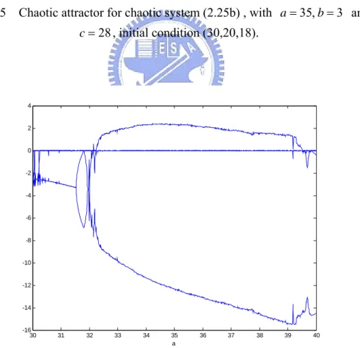
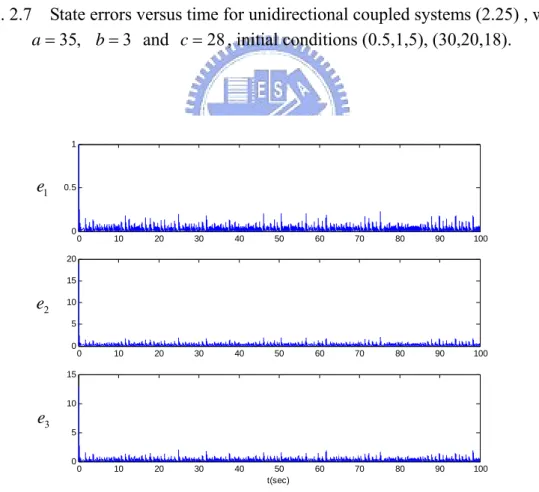
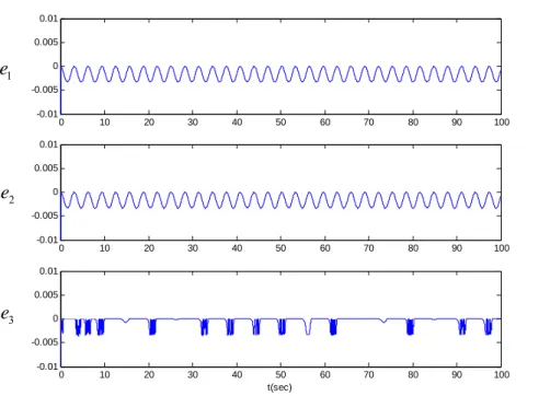
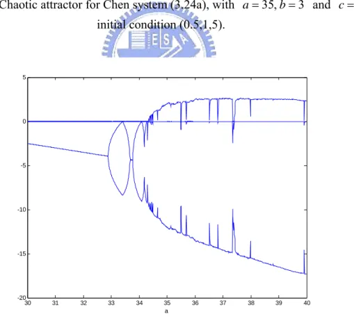
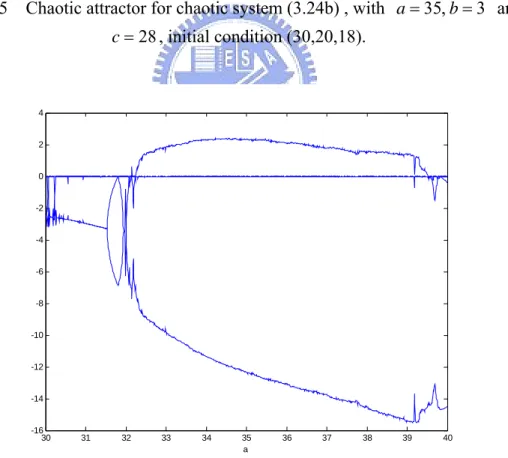
where 300γ = which is sufficiently large. Eq. (2.25a) is Chen system and Eq. (2.25b) is a new chaotic system which we proposed. The chaotic attractor and Lyapunov exponent diagrams for system (2.25a) and (2.25b) without coupling term are shown in Fig. 2.3, Fig. 2.4, Fig. 2.5 and Fig. 2.6. For initial states (0.5,1,5), (30,20,18) and system parameters a=35,b= and 3 c=28, three state errors versus time are shown in Fig. 2.7 and Fig. 2.8. Fig. 2.7 shows that state errors decreases with time when state error is large, but one can clearly find in Fig. 2.8 that the errors cannot approach zero as time evolves.

An example for the second theorem is Rössler system with a new chaotic system proposed. Consider the following unidirectional coupled systems with linear coupling in the form of Eq. (2.5):

( ) x y z y x ay z b z x c = − − = + = + − (2.26a) 2 2 2 sin ( ) sin ( ) ( ) sin ( ) x y z y x x y x ay y y y z b z x c z z z γ γ γ = − − − + − = + − + − = + − − + − (2.26b)

where 300γ = . The Lyapunov exponent diagrams for system (2.26a) and (2.26b) without coupling term are shown in Fig. 2.9 and Fig. 2.10. For initial states (20,10,25), (2.5,2,2.5) and system parameter a=0.2,b=0.2 and c=5.7, three state errors versus time are shown in Fig. 2.11. Fig. 2.11 shows that state errors decreases with time when state error is large, but one can clearly find that the errors cannot approach zero as time evolves.

chaotic system proposed for n=2. Consider the following unidirectional coupled systems with linear coupling in the form of Eq. (2.5):

1 2 3 2 2 1 1 cos x x x δx αx βx a ωt = = − + − + (2.27a) 1 2 1 1 3 2 2 2 1 1 2 2 2 ( ) cos 0.05 ( ) x x x x x x x x a t x x x γ δ α β ω γ = + − = − + − + − + − (2.27b)

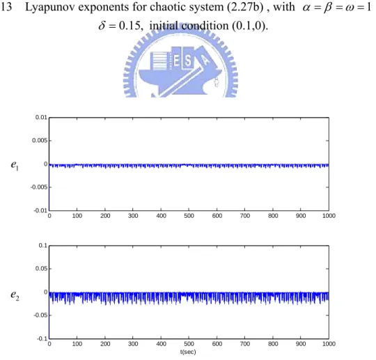
where 30γ = . The chaotic attractor and Lyapunov exponent diagrams for system (2.27a) and (2.27b) without coupling term are shown in Fig. 2.12 and Fig. 2.13. For initial states (2,2), (0.1,0) and system parameters δ =0.15, α β ω= = = and 1

3

a= , three state errors versus time are shown in Fig. 2.14. Fig. 2.14 shows that state errors decreases with time when state error is large, but one can clearly find that the errors cannot approach zero as time evolves.

2.4 Summary

In this Chapter two theorems which give the criteria of unsynchronizability for two different chaotic dynamic systems are presented. A sufficient criterion for synchronization is enhanced to necessary and sufficient one. Three simulated examples are given to illustrate the theory.

D

o r

Fig. 2.1 D region for n=2.

o r

D

Fig. 2.2 D region for n=2.

1 e 2 e 1 e 1 e 2 e

-30 -20 -10 0 10 20 30 -30 -20 -10 0 10 20 30 40 0 20 40 60 x y z

Fig. 2.3 Chaotic attractor for Chen system (2.25a), with a=35,b= and 3 c=28, initial condition (0.5,1,5). 30 31 32 33 34 35 36 37 38 39 40 -20 -15 -10 -5 0 5 a

Fig. 2.4 Lyapunov exponents for Chen system (2.25a), with b=3 and c=28, initial condition (0.5,1,5).

-30 -20 -10 0 10 20 30 40 -60 -40 -20 0 20 40 0 20 40 60 80 100 120 140 y x z

Fig. 2.5 Chaotic attractor for chaotic system (2.25b) , with a=35,b= and 3 28 c= , initial condition (30,20,18). 30 31 32 33 34 35 36 37 38 39 40 -16 -14 -12 -10 -8 -6 -4 -2 0 2 4 a

Fig. 2.6 Lyapunov exponents for chaotic system (2.25b) , with b=3 and c=28, initial condition (30,20,18).

0 0.05 0.1 0.15 0.2 0.25 0.3 0.35 0.4 0.45 0.5 0 10 20 30 0 0.05 0.1 0.15 0.2 0.25 0.3 0.35 0.4 0.45 0.5 0 5 10 15 20 0 0.05 0.1 0.15 0.2 0.25 0.3 0.35 0.4 0.45 0.5 0 5 10 15 t(sec)

Fig. 2.7 State errors versus time for unidirectional coupled systems (2.25) , with 35,

a= b=3 and c=28, initial conditions (0.5,1,5), (30,20,18).

0 10 20 30 40 50 60 70 80 90 100 0 0.5 1 0 10 20 30 40 50 60 70 80 90 100 0 5 10 15 20 0 10 20 30 40 50 60 70 80 90 100 0 5 10 15 t(sec)

Fig. 2.8 State errors versus time for unidirectional coupled systems (2.25) , with 35, 3

a= b= and c=28, initial conditions (0.5,1,5), (30,20,18).

1 e 3 e 2 e 3 e 2 e 1 e

0 0.05 0.1 0.15 0.2 0.25 -6 -5 -4 -3 -2 -1 0 1 a

Fig. 2.9 Lyapunov exponents for Rössler system (2.26a), with b=0.2 and c=5.7, initial condition (20,10,25). 0 0.05 0.1 0.15 0.2 0.25 -0.02 0 0.02 0.04 0.06 0.08 0.1 0.12 a

Fig. 2.10 Lyapunov exponent for chaotic system (2.26b) , with b=0.2 and 5.7

0 10 20 30 40 50 60 70 80 90 100 -0.01 -0.005 0 0.005 0.01 0 10 20 30 40 50 60 70 80 90 100 -0.01 -0.005 0 0.005 0.01 0 10 20 30 40 50 60 70 80 90 100 -0.01 -0.005 0 0.005 0.01 t(sec)

Fig. 2.11 State errors versus time for unidirectional coupled systems (2.26) , with 0.2, 0.2

a= b= and c=5.7, initial conditions (20,10,25), (2.5,2,2.5).

0 0.5 1 1.5 2 2.5 3 -0.4 -0.3 -0.2 -0.1 0 0.1 0.2 0.3 a

Fig. 2.12 Lyapunov exponents for Duffing system, with α β ω= = = and 1 0.15, δ = initial condition (2,2). 1 e 3 e 2 e

0 0.5 1 1.5 2 2.5 3 -0.4 -0.3 -0.2 -0.1 0 0.1 0.2 0.3 a

Fig. 2.13 Lyapunov exponents for chaotic system (2.27b) , with α β ω= = = and 1 0.15, δ = initial condition (0.1,0). 0 100 200 300 400 500 600 700 800 900 1000 -0.01 -0.005 0 0.005 0.01 0 100 200 300 400 500 600 700 800 900 1000 -0.1 -0.05 0 0.05 0.1 t(sec)

Fig. 2.14 State errors versus time for unidirectional coupled systems (2.27) , with 0.15,

δ = α β ω= = = and 1 a=3, initial conditions (2,2), (0.1,0).

1

e

2

Chapter 3

Two Theorems of Generalized Unsynchronization for

Coupled Chaotic Systems

3.1 Preliminary

In this Chapter, we propose two theorems which give the criteria of generalized unsynchronization for two different chaotic dynamic systems with whatever large strength of linear coupling. Chen system and a new chaotic system which we proposed are presented as a simulated example for the first theorem. Rössler system with corresponding new chaotic system proposed are presented as simulated examples for the second theorem.

3.2 Two Theorems of Generalized Unsynchronizability

Consider the following nonautomonous systems ( , )t = x f x (3.1) where ∈ n x R , : ₁ n n + Ω ⊂ × →

f R R R . Eq. (3.1) is considered as a master system. A

slave system is given by ( , )t = y g y (3.2) where ∈ n y R , : ₂ n n + Ω ⊂ × →

g R R R . Both f and g satisfy Lipschitz condition.

1

Ω , Ω are domains containing the origin. Assume that the solutions of Eqs. (3.1) 2

and (3.2) have bounds then they must exist for infinite time.

Now we consider the following unidirectional nonautonomous coupled system ( , ) ( , ) ( , , ) t t t = = + x f x y g y U x y (3.3)

Definition The system (3.3) is generalized synchronized if there is a continuous

function H x and let error ( ) e y= −H( )x s.t. lim 0

t→∞ e = . But, if no positive

constant C can be found such that e→0 as t→ ∞ for all e( )t0 <C, systems (3.3)

are generalized unsynchronizable.

In order to discuss the generalized synchronization of x and y , define ( )

H

=

z x and error e y z . Error equation can be written as = − ( ,t ) ∂H ( , )t ( , ,t )

= − = + − + +

∂

e y z g e z f x U z e z

x (3.4)

Now the first theorem will be given for a special case of Eqs. (3.3). Consider unidirectional coupled nonautonomous systems as

( , ) ( , ) ( ) t t = = + − x f x y g y Γ z y (3.5)

where f and g satisfy Lipschitz condition, and the Lipschitz constant of g is L .

n n

M _×

∈

Γ is a constant diagonal matrix with positive entries which represents the strength of the linear coupling term z y . Since − e y= −H( )x = −y z , the error dynamic equation can be obtained as

( ,t ) ∂H ( , )t = − = + − − ∂ e y z g e z f x Γe x (3.6) Let ( , )t =∂H ( , )t ∂ h z f x

x , system (3.6) can be written as

( ,t ) ( , )t

= − = + − −

e y z g e z h z Γe (3.7)

which is a nonautonomous system of differential equations for state e.

Theorem 3.1 Two different dynamic systems in Eq. (3.5) are of generalized

unsynchronizability for however large coupling strength Γ with positive entries, if ( , ) ( , )

i i

h t z ≤g t z (i= …1, , )n in Ω1∩Ω2, and h z( , )t −g z( , )t >0 except at origin,

Proof. Choose a Lyapunov function V( )e =e e1 2 en which is positive in quadrant

1 0, 2 0, , n 0

e > e > e > , then V along any state trajectory of system (3.6) becomes

[25]: 2 3 1 1 3 2 1 2 1 2 3 1 1 1 1 1 3 2 2 2 2 1 2 1 2 3 1 1 1 1 1 1 1 2 1 [ ( , ) ( , ) ] [ ( , ) ( , ) ] [ ( , ) ( , ) ] [ ( , ) ( , ) ( , ) ( , ) ] [ n n n n n n n n n n n n n V e e e e e e e e e e e e e e e g t h t e e e e g t h t e e e e g t h t e e e e g t g t g t h t e e e e g − − − = + + + = + − − Γ + + − − Γ + + − − Γ = + − + − − Γ + + e z z e z z e z z e z z z z ( , ) ( , ) ( , ) ( , ) ] n t e z+ −g tn z +g tn z −h tn z − Γn ne When e1>0,e2 >0, ,en > , we have 0 2 3 1 1 1 1 1 1 1 2 1 2 3 1 1 1 1 [ ( , ) ( , ) ( , ) ( , ) ] [ ( , ) ( , ) ( , ) ( , ) ] [ ( , ) ( , ) ] n n n n n n n n n V e e e g t g t g t h t e e e e g t g t g t h t e e e e L g t h t e − ≤ + − + − − Γ + + + − + − − Γ ≤ + − − Γ + e z z z z e z z z z e z z (3.8) where g t₁( ,e z+ −) g t₁( , )z ≤L e follows the Lipschitz condition. When e 1,

the terms of lower degree of error components e e2 3 e g tn[ ( , )1 z −h t1( , )]z , 1 3 n[ ( , )2 2( , )]

e e e g t z −h t z , can be neglected when the sign of V is considered,

then

2 3 n[ 1 1] 1 3 n[ 2 2]

V ≤e e e L e − Γe +e e e L e − Γ e + (3.9)

For sufficient large Γ , V can be negative in the quadrant _i e₁> , 0 e₂ > , 0 ,

0

n

e > . So the state point tends to decrease e( )t with time when e₀ is sufficiently large. When e 1 , the proof is as follows. Now when

1 0, 2 0, , n 0 e > e > e > , V is expressed as 2 3 1 1 1 1 1 1 2 3 1 1 1 1 [ ( , ) ( , ) ( , ) ( , ) ] [ ( , ) ( , ) ] n n V e e e g t g t g t h t e e e e L g t h t e ≥ − + − + − − Γ + ≥ − + − − Γ + e z z z z e z z (3.10)

When e 1, the terms of higher degree e e_{2 3} en[−L e − Γ_{1 1}e], can be neglected when the sign of V is considered, then

2 3 n[ ( , )1 1( , )] 1 3 n[ ( , )2 2( , )]

V ≥e e e g t z −h t z +e e e g t z −h t z + (3.11)

By the condition ( , )h t_i z ≤g t_i( , )z (i= …1, , )n inΩ1∩Ω2 , h z( , )t −g z( , )t >0 ,

( , ) ( , )

i i

f t z =g t z (i=1, , )n do not occur simultaneously. Therefore the right-hand

side of above inequality is positive, i.e. V is positive in region D of Fig. 3.1, which is the quadrant e₁> , 0 e₂ > , 0 , 0e_n > of the neighborhood of the origin.

Choose r>0 such that for the ball B_r = ∈{e Rn e ≤r}, we have

{ r ( ) 0}

D= ∈e B V e > (3.12)

of which the boundary is the surface V( ) 0e = and the sphere e =r . Since ( ) 0

V 0 = , the origin lies on the boundary of D inside B . The point _r e is in the ₀

interior of D and V( )e₀ = >b 0. Now we prove that the trajectory e( )t started at

0

(0)=

e e must leave the set D, i.e. the trajectory must leave the neighborhood of

origin, e cannot approach zero. To see this point, notice that as long as ( )e t is

inside D, ( ( ))V e t ≥b since ( ) 0V e > in D. Let

min{ ( )V D and V( ) b}

β = e e∈ e ≥ (3.13)

which exists since the continuous function ( )V e has a minimum over the compact

set {e∈D and V( )e ≥b}= ∈{e B and V_r, ( )e ≥b} [29]. Then, β > and 0

0 _{0 0}

( ( )) ( ) t ( ( )) t

V e t =V e +

∫

∫

This inequality shows that ( )e t cannot stay forever in D because ( )V e is bounded

on D. Now, ( )e t cannot leave D through the surface ( ) 0V e = since ( ( ))V e t ≥b.

are unsynchronizable for however large Γ .

Theorem 3.2 Two different dynamic systems in Eq. (3.5) are of generalized

unsynchronizability for however large coupling strength Γ , if ( , )h ti z ≥g ti( , )z (i= …1, , )n in Ω1∩Ω2, and h z( , )t −g z( , )t >0 except at origin, for any solution

( )t

z .

Proof. Choose a Lyapunov function V( )e =e e_{1 2} e_n , then V along any state

trajectory of system (3.6) becomes:

Case 1. When n is odd, V e is negative in quadrant ( ) e₁<0,e₂<0, e_n < . 0

2 3 1 1 3 2 1 2 1 2 3 [ ( ,1 ) 1( , ) 1( , ) 1( , ) 1 1] 1 2 1[ ( , ) ( , ) ( , ) ( , ) ] n n n n n n n n n n n n V e e e e e e e e e e e e e e e g t g t g t h t e e e e g t g t g t h t e − − = + + + = + − + − − Γ + + + − + − − Γ e z z z z e z z z z When e1<0,e2<0, en < , we have 0 2 3 1 1 1 1 1 1 1 2 1 2 3 1 1 1 1 [ ( , ) ( , ) ( , ) ( , ) ] [ ( , ) ( , ) ( , ) ( , ) ] [ ( , ) ( , ) ] n n n n n n n n n V e e e g t g t g t h t e e e e g t g t g t h t e e e e L g t h t e − ≥ − + − + − − Γ + + − + − + − − Γ ≥ − + − − Γ + e z z z z e z z z z e z z (3.15) where g t₁( ,e z+ −) g t₁( , )z ≤L e follows the Lipschitz condition. When e 1,

the terms of lower degree of error components e e2 3 e g tn[ ( , )1 z −h t1( , )]z , 1 3 n[ ( , )2 2( , )]

e e e g t z −h t z , can be neglected when the sign of V is considered,

then 2 3 1 1 1 3 2 2 2 3 1 1 1 3 2 2 [ ] [ ] [ ] [ ] n n n n V e e e L e e e e L e e e e L e e e e L e ≥ − − Γ + − − Γ + = − + Γ − + Γ + e e e e (3.16)

For sufficient large Γ , V can be positive in the quadrant _i e₁ < , 0 e₂< , 0 ,

0

n

sufficiently large. When e 1, the proof is as follows. Now when e₁< 0, e₂ < 0, 0 n e < , V is expressed as 2 3 1 1 1 1 1 1 2 3 1 1 1 1 [ ( , ) ( , ) ( , ) ( , ) ] [ ( , ) ( , ) ] n n V e e e g t g t g t h t e e e e L g t h t e ≤ + − + − − Γ + ≤ + − − Γ + e z z z z e z z (3.17)

When e 1, the terms of higher degree e e_{2 3} e Ln[ e − Γ_{1 1}e], can be neglected when the sign of V is considered, then

2 3 n[ ( , )1 1( , )] 1 3 n[ ( , )2 2( , )]

V ≤e e e g t z −h t z +e e e g t z −h t z + (3.18)

By the condition h z( , )t −g z( , )t >0, ( , )h t_i z =g t_i( , )z (i=1, , )n do not occur

simultaneously. Therefore the right-hand side of above inequality is negative, i.e. V is negative in region D of Fig. 3.2, which is the quadrant e1< , 0 e2 < , 0 , 0en <

of the neighborhood of the origin.

Choose r>0 such that for the ball B_r = ∈{e Rn e ≤r}, we have

{ r ( ) 0}

D= ∈e B V e < (3.19)

By the similar reasoning as that in the latter part of the proof for Theorem1, we can prove that the state trajectory started from D must leave the neighborhood of the origin, e can never approach zero. Two different dynamic systems in Eq. (3.5) are unsynchronizable for however large Γ .

Case 2. When n is even, V e is positive in quadrant ( ) e₁<0,e₂ <0, e_n < . 0

2 3 1 1 3 2 1 2 1 2 3 [ ( ,1 ) 1( , ) 1( , ) 1( , ) 1 1] 1 2 1[ ( , ) ( , ) ( , ) ( , ) ] n n n n n n n n n n n n V e e e e e e e e e e e e e e e g t g t g t h t e e e e g t g t g t h t e − − = + + + = + − + − − Γ + + + − + − − Γ e z z z z e z z z z When e1<0,e2<0, en < , we have 0

2 3 1 1 1 1 1 1 1 2 1 2 3 1 1 1 1 [ ( , ) ( , ) ( , ) ( , ) ] [ ( , ) ( , ) ( , ) ( , ) ] [ ( , ) ( , ) ] n n n n n n n n n V e e e g t g t g t h t e e e e g t g t g t h t e e e e L g t h t e − ≤ − + − + − − Γ + + − + − + − − Γ ≤ − + − − Γ + e z z z z e z z z z e z z (3.20) where g t1( ,e z+ −) g t1( , )z ≤L e follows the Lipschitz condition. When e 1,

the terms of lower degree of error components e e_{2 3} e g t_n[ ( , )₁ z −h t₁( , )]z ,

1 3 n[ ( , )2 2( , )]

e e e g t z −h t z , can be neglected when the sign of V is considered,

then 2 3 1 1 1 3 2 2 2 3 1 1 1 3 2 2 [ ] [ ] [ ] [ ] n n n n V e e e L e e e e L e e e e L e e e e L e ≤ − − Γ + − − Γ + = − + Γ − + Γ + e e e e (3.21)

For sufficient large Γ , V can be negative in the quadrant i e1< , 0 e2 < , 0 ,

0

n

e < . So the state point tends to decrease e( )t with time when e0 is

sufficiently large. When e 1, the proof is as follows. Now when e1< , 0 e2 < , 0

, 0en < , V is expressed as 2 3 1 1 1 1 1 1 2 3 1 1 1 1 [ ( , ) ( , ) ( , ) ( , ) ] [ ( , ) ( , ) ] n n V e e e g t g t g t h t e e e e L g t h t e ≥ + − + − − Γ + ≥ + − − Γ + e z z z z e z z (3.22)

When e 1, the terms of higher degree e e2 3 e Ln[ e − Γ1 1e], can be neglected

when the sign of V is considered, then

2 3 n[ ( , )1 1( , )] 1 3 n[ ( , )2 2( , )]

V ≥e e e g t z −h t z +e e e g t z −h t z + (3.23)

By the condition h z( , )t −g z( , )t >0, ( , )h t_i z =g t_i( , )z (i=1, , )n do not occur

simultaneously. Therefore the right hand side of above inequality is positive, i.e. V is positive in region D of Fig. 3.2 which is the quadrant e₁< , 0 e₂ < , 0 , 0e_n <

By the same reasoning as that in the latter part of the proof for Theorem 1, we can prove that the state trajectory started from the neighborhood of the origin in the quadrant e1< , 0 e2 < , 0 , 0en < must leave the neighborhood and can never

approach zero. Two different dynamic systems in Eq. (3.5) are unsynchronizable for however large Γ . i

3.3 Simulated Examples

An example for the first theorem is Chen system with a new chaotic system proposed. Consider the following unidirectional coupled systems:

( ) ( ) x a y x y c a x xz cy z xy bz = − = − − + = − (3.24a) 2 1 2 2 2 3 ( ) sin ( ) x a y x x e y c a x xz cy x e z xy bz x e γ γ γ = − + − = − − + + − = − + − (3.24b) = − e y z , z=H( )x =Ax b + 1 0 0 0 1 0 0 0 1 ⎡ ⎤ ⎢ ⎥ = ⎢ ⎥ ⎢ ⎥ ⎣ ⎦ A , 3 5 7 ⎡ ⎤ ⎢ ⎥ = ⎢ ⎥ ⎢ ⎥ ⎣ ⎦ b

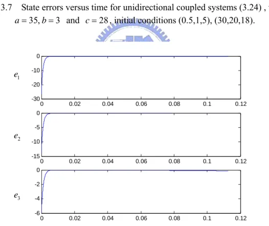
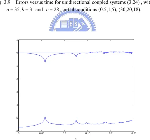
where 1000γ = which is sufficiently large. Eq. (3.24a) is Chen system and Eq. (3.24b) without coupling is a new chaotic system which we proposed. The chaotic attractor and Lyapunov exponent diagrams for system (3.24a) and (3.24b) without coupling term are shown in Figs. 3.3 ~ 3.6. For initial states (0.5,1,5), (30,20,18) and system parameters a=35,b= and 3 c=28, three state errors and error versus time are shown in Figs. 3.7 ~ 3.9. Fig. 3.8 shows that errors decreases with time when error is large, but one can clearly find in Fig. 3.9 that the errors cannot approach zero as time evolves.

An example for the second theorem is Rössler system with a new chaotic system proposed. Consider the following unidirectional coupled systems with linear coupling in the form of Eq. (3.5):

( ) x y z y x ay z b z x c = − − = + = + − (3.25a) 2 1 2 2 2 3 sin sin ( ) sin x y z y e y x ay y e z b z x c z e γ γ γ = − − − − = + − − = + − − − (3.25b) = − e y z , z=H( )x =Ax b + 1 0 0 0 1 0 0 0 1 ⎡ ⎤ ⎢ ⎥ = ⎢ ⎥ ⎢ ⎥ ⎣ ⎦ A , 3 5 7 ⎡ ⎤ ⎢ ⎥ = ⎢ ⎥ ⎢ ⎥ ⎣ ⎦ b

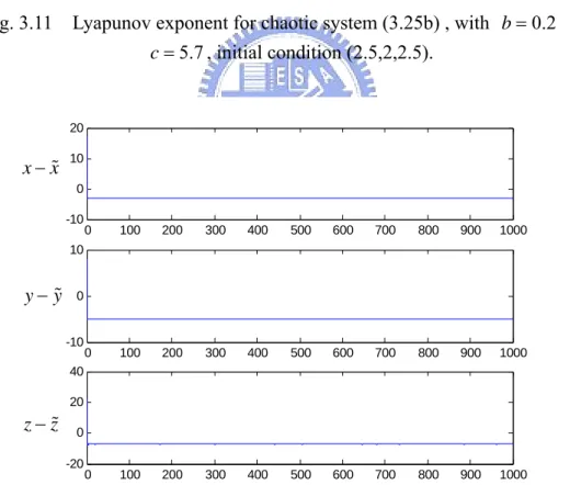
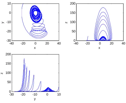
where 300γ = . The Lyapunov exponent diagrams for system (3.25a) and (3.25b) without coupling term are shown in Figs. 3.10 ~ 3.11. For initial states (20,10,25), (2.5,2,2.5) and system parameter a=0.2,b=0.2 and c=5.7, three state errors and errors versus time are shown in Figs. 3.12 ~ 3.14. Fig. 3.13 shows that errors decreases with time when error is large, but one can clearly find in Fig. 3.14 that the errors cannot approach zero as time evolves.

3.4 Summary

In this Chapter, two theorems are proposed. They give the criteria of generalized unsynchronization for two different chaotic dynamic systems with whatever large strength of linear coupling. Chen system and Rössler system with two corresponding new chaotic systems proposed are used as simulation examples which effectively confirm the theorems.

D

o r

Fig. 3.1 D region for n=2.

o r

D

Fig. 3.2 D region for n=2.

1 e 2 e 1 e 1 e 2 e

-30 -20 -10 0 10 20 30 -30 -20 -10 0 10 20 30 40 0 20 40 60 x y z

Fig. 3.3 Chaotic attractor for Chen system (3.24a), with a=35,b= and 3 c=28, initial condition (0.5,1,5). 30 31 32 33 34 35 36 37 38 39 40 -20 -15 -10 -5 0 5 a

Fig. 3.4 Lyapunov exponents for Chen system (3.24a), with b=3 and c=28, initial condition (0.5,1,5).

-30 -20 -10 0 10 20 30 40 -60 -40 -20 0 20 40 0 20 40 60 80 100 120 140 y x z

Fig. 3.5 Chaotic attractor for chaotic system (3.24b) , with a=35,b= and 3 28 c= , initial condition (30,20,18). 30 31 32 33 34 35 36 37 38 39 40 -16 -14 -12 -10 -8 -6 -4 -2 0 2 4 a

Fig. 3.6 Lyapunov exponents for chaotic system (3.24b) , with b=3 and c=28, initial condition (30,20,18).

0 50 100 150 200 250 300 -10 -5 0 0 50 100 150 200 250 300 -10 -5 0 0 50 100 150 200 250 300 -15 -10 -5

Fig. 3.7 State errors versus time for unidirectional coupled systems (3.24) , with 35, 3

a= b= and c=28, initial conditions (0.5,1,5), (30,20,18).

0 0.02 0.04 0.06 0.08 0.1 0.12 -30 -20 -10 0 0 0.02 0.04 0.06 0.08 0.1 0.12 -15 -10 -5 0 0 0.02 0.04 0.06 0.08 0.1 0.12 -6 -4 -2 0

Fig. 3.8 Errors versus time for unidirectional coupled systems (3.24) , with a=35, 3

b= and c=28, initial conditions (0.5,1,5), (30,20,18). x−x y− y z− z 1 e 2 e 3 e

0 50 100 150 200 250 300 -30 -20 -10 0 10 0 50 100 150 200 250 300 -20 -10 0 10 0 50 100 150 200 250 300 -10 -5 0 5

Fig. 3.9 Errors versus time for unidirectional coupled systems (3.24) , with 35, 3

a= b= and c=28, initial conditions (0.5,1,5), (30,20,18).

0 0.05 0.1 0.15 0.2 0.25 -6 -5 -4 -3 -2 -1 0 1 a

Fig. 3.10 Lyapunov exponents for Rössler system (3.25a), with b=0.2 and 5.7 c= , initial condition (20,10,25). 1 e 2 e 3 e

0 0.05 0.1 0.15 0.2 0.25 -0.02 0 0.02 0.04 0.06 0.08 0.1 0.12 a

Fig. 3.11 Lyapunov exponent for chaotic system (3.25b) , with b=0.2 and 5.7 c= , initial condition (2.5,2,2.5). 0 100 200 300 400 500 600 700 800 900 1000 -10 0 10 20 0 100 200 300 400 500 600 700 800 900 1000 -10 0 10 0 100 200 300 400 500 600 700 800 900 1000 -20 0 20 40

Fig. 3.12 State errors versus time for unidirectional coupled systems (3.25) , with 0.2, 0.2

a= b= and c=5.7, initial conditions (20,10,25), (2.5,2,2.5). x−x

y− y

0 0.05 0.1 0.15 0.2 0.25 0 10 20 30 0 0.05 0.1 0.15 0.2 0.25 -10 0 10 20 0 0.05 0.1 0.15 0.2 0.25 -20 0 20 40

Fig. 3.13 Errors versus time for unidirectional coupled systems (3.25) , with 0.2, 0.2

a= b= and c=5.7, initial conditions (20,10,25), (2.5,2,2.5).

0 100 200 300 400 500 600 700 800 900 1000 0 0.5 1 0 100 200 300 400 500 600 700 800 900 1000 -0.5 0 0.5 0 100 200 300 400 500 600 700 800 900 1000 -1 0 1

Fig. 3.14 Errors versus time for unidirectional coupled systems (3.25) , with 0.2, 0.2

a= b= and c=5.7, initial conditions (20,10,25), (2.5,2,2.5).

1 e 2 e 3 e 1 e 2 e 3 e

Chapter 4

Chaos Synchronization by Variable Strength Linear

Coupling and Lyapunov Function Derivative in Series Form

4.1 Preliminary

In this Chapter, a new general strategy to achieve chaos synchronization by variable strength linear coupling is proposed. This method, in which the time derivative of Lyapunov function in series form is firstly used, can give either local synchronization which is usually good enough or global synchronization which is usually an unnecessary high demand.

4.2 Synchronization Strategy by Variable Strength Linear Coupling and Lyapunov Function Derivative in Series Form

(a) Consider the following unidirectional coupled identical chaotic systems ( ) ( ) ( ) = + = + + − x Ax f x y Ay f y Γ y x (4.1) where

[

]

[

]

y denote two state vectors,

A is an n n× constant coefficient matrix, f is a nonlinear vector function, and Γ is an n n× matrix which gives the variable strength of the linear coupling term

(y x . − )

In order to study the synchronization of x and y , define = −e y x as the state

error. Error equation can be written as

( ) ( ) ( ) = + + − − − e Ay f y Γ y x Ax f x (4.2) By Taylor expansion HOT of HOT of ′ + = + f(y) - f(x) = f(x + e) - f(x) = f (x)e e F(x)e e (4.3)