Control design for vehicle's lateral dynamics

2006IEEEInternational Conferenceon

Systems, Man, andCybernetics October8-11,

2006,

Taipei, Taiwan

Control Design for

Vehicle's Lateral

Dynamics

Der-Cheng Liaw and Wen-Ching Chung

Abstract-issuesofcontrollability and stabilization design for

vehicle's lateral dynamics are presented. Based on the

assumption ofconstantdrivingspeed,asecond-order nonlinear

lateral dynamical model is obtained. It is observedthatsaddle

nodebifurcation will appear in vehicledynamicswith respectto

the variation of the front wheel steering angle, which might

result in spin and/or system instability. In order to possibly

prevent the occurrenceof suchaninstability,thecontrollability

of vehicle dynamics at the saddle node bifurcation point is

discussed. This leads to the design ofa direct state feedback

control law for systemstabilization.Two-Parameterbifurcation

analysis of system behavior is also obtained to classify the

regime of the effective control gains for system stabilization.

Numerical simulations foran example model demonstrate the

effectiveness ofanalyticalresults. I. INTRODUCTION

ecently,thestudyof thevehicle'sdynamicshasattracted onsiderableattention [1]-[6].Oneofthemajor goalsof thosestudiesistoenhancethedriving safetysince there have huge amountoftraffic accidentsoccurring indaily life. Itis knownthat thosetraffic accidentsarehighlyrelatedwith the nonlinear behaviorofvehicledynamics.Thelinkagebetween the nonlinearphenomenaofvehicledynamics andthe

applied

frontwheel steering anglehence becomesa veryimportant issue. Amongthoseexisting studies, slidingmodeapproach has been used to design robust control laws for providing systemstabilitywith respecttothelarge variation of system parameterssuchasaxialvelocity,massofthevehicleand the

contact force between tire and road surface [2]. A five degree-of-freedom vehicle modelwasused in[6]todesignan

extended Kalmanfilter(EKF) forestimatingthehistoricdata ofvehicle'smotionandcorrespondingtire forces.Basedon a

linearmodel ofvehicle's lateraldynamics,linearcontrol laws have been proposed in [3, 4]. Saddle-node bifurcation was

observed in vehicle dynamics [5] to link with system instability via a numerical example. Such a bifurcation phenomenon might result inspinof the vehicle.

Bifurcation theory and itsapplicationshave beenrecently wellexploited[7]-[11]. Byapplyingthebifurcation theory, a theoreticalanalysisof vehicledynamicshas beenobtained by Liawetal[12], whichrevealedthat theuncontrolledmodel of

Manuscriptreceived March 15, 2006. This workwassupportedinpartby theMinistryofEducation,Taiwan,R.O.C. under Grant EX-9 1 -E-FA06-4-4.

Der-Chemg Liaw, Corresponding author, Professor, Department of

Electrical and Control Engineering, National Chiao Tung University, Hsinchu 300, Taiwan, R.O.C. (phone: +886-3-5712121-54363; fax:

+886-3-5715998;e-mail:[email protected]).

Wen-Ching Chung, Ph.D. Candidate, Department of Electrical and

Control Engineering,National ChiaoTungUniversity,Hsinchu300,Taiwan, R.O.C.

vehicle's lateral dynamics might undergo stationary saddle nodebifurcation.

In this paper, we continue the study of vehicle's lateral dynamicsasthat in [12] butfocusonthe control issue. Here, weconsiderthe nonlinear model ofvehicle'slateraldynamics byassumingconstantvelocityinmotion equationsof steering dynamics withoutconsideringroll motion. In order to find the existence conditions of stabilization controller, system controllability at saddle node bifurcation point will be

first

discussed. Feedback control design will thenbe studied for preventing or delaying the appearance of saddle node bifurcation.

Thepaper isorganizedasfollows.Mathematical models of vehicle system arerecalledinSection

II.

Itisfollowed by the analysis of existence and stability conditions for system equilibrium. The study ofcontrollability atthe saddlenode bifurcationpoint and direct state feedback control design is given in Section IV. Finally,numericalstudies for an example carmodelaregiveninSectionVtodemonstrate theanalytical results.

II. VEHICLE DYNAMICS

In the following, we recall the mathematical model for vehicle'ssteeringdynamicsfrom

[1],

which will beemployed inthe paper.

Consider the vehicle's steeringdynamicsasdepictedinFig. 1(e.g.,

[1],

[12]). Letboth sideslipangle

,dand

yaw rate y be system outputs for the steering characteristics and the front-wheel angle

Sf

be only system input. In addition,

Lf

denote the length between the center of gravity (CG) and front-wheel axes and

Lr

denote the length between CG and rear-wheel axes, respectively. Moreover,

Fyfl

and

Fyri

(resp.

Fyfr

and

Fyrr)

aretheleft-side (resp.right-side)comering force offronttires andreartires,and bothFxfland FXfr (resp. FXfrand

Fxrr)

are the left-side (resp. right-side) traction force of front andreartires. Forsimplicity andwithout loss ofgenerality, here, we assume the vehicle body is symmetric about the longitudinalplane. Let

Fyf

=

Fyfl

+

Fyjr,

Fyr=

Fyrl

+

Fyrr,

FXj=

Ffl

+

Fxfr

and

Fxr

=

Flri

+

Fxrr.

Thebasic motion equations for

steeringdynamicswith roll motionneglected was derived in

[1]

asgiven by

m(v

v,3r)

=F +

\,

Fy,

sin

S1,'

(1)

mv (,B+

r)

=

Fyf

+

Fyr

+ fsin

'if

, (2)

(3)

Iz=

(LFy

-LrFyr)

cos/8+LjFIf

sin

1f,

where

m:themassof thevehicle,

I,:

theyawmomentaroundz-axis,

v:thelongitudinal velocity.

Fig. 1. Vehicle's steering dynamics.

In this study, we focus on the characteristic analysis of lateral dynamics by assuming

Ff

= 0 and there are no

accelerationordecelerationonthevehiclealonglongitudinal direction, i.e., =0 . Thus, Eq. (1) can be neglected for

analysis.Thesteering dynamicsforconstantspeedv canthen be reducedto asecond-order modelasgiven by

/-4(13,y,

j)

-vIF,

+

Fy,.

}-y, (4)

Yf2(A/3V4)

I1

{LfF1§

L,F

}

cos/,

(5) whereboth

Fyf

andFyr areknown functions of /1, r and

f.

III. STABILITY ANALYSIS

Inthissection,weadopt the second-order modelasinEqs. (4)-(5) to study the local stability for the vehicle's steering dynamics. Denote x

=(,80,y0°)T

an equilibrium point of

system(4)-(5)foragiven steeringwheelangle

3f

=

fj°.

By

the definition ofequilibrium point,wethen have

Fyf(

,0y

00f)+

(Po,

70,sf

a

=y°mv

(6)

and L

Fyf

(0,

70,

f)-

LF,,(,B°0,y0,Sf

0)=0

(7)

or

cos,0

=0.

(8)

Tocheck thecondition ofEq.(8),wehave /30 nir+ % for

n=0, 1, 2,... It is clear that avehicle can not

easily

achieve such acondition. Thus, the equilibrium point

xo

ingeneral shouldsatisfy the conditions of Eqs. (6) and (7).

Let

x=(,B,7)T,

x=x-

xo

and control inputu= 5 -b°0 .

Takingthelinearization ofsystem(4)-(5)at

xo

and

5f

=05f°,

wehave x=

Aix

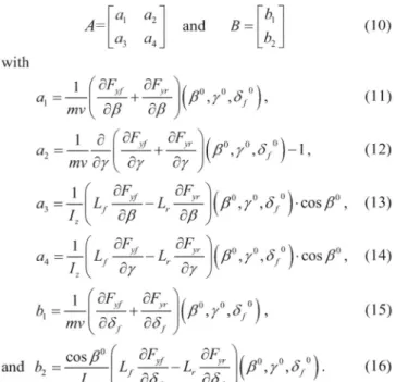
+Bu, where A=

[,

a2 and B

K]b,

LA a4j b2 with mvK a>

7(o)

a2

=--

y°,

)1,__I

mvayya7 a7 ' a3

(Lf-

Lr-)

3° y°,

P

f

°)-cosfl,

aF

aF>0\

a4 I-L (ao)-cos30,pY

Kl

=-

0d2

+ (°/ J)0 ns1)ias1 ( oyoo)

and

b2

cs3LfY

LrJ(/3

Y0(i0)

(10) (11) (12) (13) (14) (15) (16)

Byapplying the Routh-Hurwitzstability criterion, we then

have the following stability result.

Lemma 1. The equilibrium point

xo

of system (4)-(5) is

asymptotically stable if

a,

+a4 <0 and

aa4-

a2a3

>0

where

ai's

aregiven in Eqs. (1I )-(14).

It is known from the so-called "Magic formula" (e.g.,

[5]-[6]) that both values of

a,

and a4, in general, will be negative. Therefore, the stability condition of

a,

+ a4 <0 is

always satisfied.An example of

ai's

willbe given in Section

V. Thus, the stability condition in Lemma 1 can then be reduced to that the equilibrium point x° ofsystem (4)-(5) will be stable if a1a4

-a2a,

>0 . It is clear from

al

+a4 <0that the linearization system(4)-(5)at x° willnot

haveapairofpureimaginary eigenvalues withrespect tothe variation of,. Instead, the systemdynamics might have one zero eigenvalue. This implies that the lateral dynamics of vehicle systemwill notundergoHopfbifurcation but might have chance for the appearance ofstationary bifurcation at some

Q-f=47f

suchthat a1a4

-a2a3

0O .

The conditions of the appearance of saddle node

bifurcation for system (4)-(5)have been obtained in [12] as

follows.

Lemma 2. The system (4)-(5) will undergo saddle node bifurcation for the equilibrium point

xo

if the following conditions hold:

(i)

a,a4= a2a3

with

a1

<0 and a4<0 (17) (9) (ii)

a4b1

.

a,b2

,and

2 2

(iii)

a4q,

1 -a3ql2

+i--q13-

a2q2,1+aq22 --q23.0,

a4 a2

(18) (19)

where qI=

f (

xo

°)

q,2

= aA

(Xa)

0

q,3 a2= (X2,s10), q 2 (X ,sj)

q22- a (x I ) and q23-

aj2

x ,9

IV. DESIGNOFSTABILIZATION CONTROL LAWS

Asgiven in Lemma2above,system(4)-(5)couldundergo stationary saddlenodebifurcation,whichmightresult inspin of vehicle. In order to prevent the appearance of such an

instability, in this sectionwe will seek forpossible control laws for system stabilization. First, we will discuss the controllabilityof system(4)-(5). Itis followedbythe design ofcontrollaws forpreventingand/ordelayingtheappearance of saddle nodebifurcation. Detailsaregivenasfollows.

A. ControllabilityAnalysis

First, we check the controllability of system (4)-(5). Denote Cthecontrollability matrix of the linearizedmodelof system(4)-(5)asgivenin(9).Wethen have

c [B AB] (20)

Fbi

ab,

+

a2b2

(21)

Lb2

a3b,

+a4b2

The determinant of the controllability matrix C is calculatedas

system stabilization. Let the control input u=K x, where K=[-k, -k2]. Thelinearized model(9)canthenrewritten

as

(24) Thecharacteristic equationof system(24) gives

22+A+h2 =

0,

where

=

klb,

+

k2b2

-a, -a4,

and h2 =aa4-a2a3+

(a2b2

-a4b,)k,

+(a3b,

-a,b2)k2.

(25) (26) (27) Byapplying theRouth-Hurwitz stabilitycriterion,wethen have the following stabilization result for the equilibrium point x°.

Theorem 1. The equilibrium point

xo

ofsystem (4)-(5) is asymptotically stabilizable if h >0 and

k

>0, where h, andh2aregiveninEqs.(26)and(27),respectively.

V. CASE STUDY

Itisknown that there are many mathematicalmodelshave beenproposed forcornering forces. In thispaper, weadopt the so-called "Magic formula" from [6] for the models of nonlinearcorneringforces

Fyf

and

Fy],

respectively, asgiven by

Fyf

=

Df

sin

[Cf

tan

1{Bf

(l-

Ef

)

af

+

Ef

tan

'(Bf

a)}

det[C]=

a3b,2

-

a2b22+

(a4

-a,) bb2.

(22)

Wehavethenextresult.

Lemma 3. The linearized model (9) is controllable at the equilibrium point

xo

if a3b

a2b2

+

(a4

-a)blb, 0,where

ai'

s and

bi's

aregiveninEqs. (11)-(16).

Next,

we study a special case ofwhich

xo

is the saddle nodebifurcation point.From[12] andLemma2inSectionIII,

wehave a,a4-a2a3=0 and

a4bj

#a2b2 when thelinearized

model is evaluatedatthe saddle nodebifurcationpoint. Eq. (22)canthen berewritten as

det

[C]

=I(a4b,

-a2b2

)(alb,

+a2b2

)

a2 (23)

The nextresult followsreadilyfrom Lemma 3.

Corollary 1. Thestationarysaddle nodebifurcationpoint

xo

of system(4)-(5)iscontrollableif

a,b,

+a2b2 .

0,

where

ai's

and

bi's

aregiveninEqs.(11)-(16).

B. StateFeedback Control Design

As discussedabove, the saddle node bifurcation point of system(4)-(5) is controllable if

a,bj

+a2b2 . 0. This leads to

the possibility of a design ofstate feedback control law for and

Fy7.

=D,sin

C,tan

{'B,.(1

-Et.)a,.+E,tan-where

a1f

=,+tan-l

j+f

y.cos;-J6f

and

ar

=

P-tan

j(-

cos/8

.

(28)

-'(Ba,.a)}],

(29)

(30) (31) Here,

Bi,

Ci, Di

and E fori =

f

rare constants.

af

and ar

denote theslipangleof front tire andreartire,respectively.It

is clear from Eqs. (28) and (29) that

(,8A

)T

=

(0,

O)T

will

make

Fyf

= Fyr-0 when

5f

=0 Thus,

xO

=(0,

O)T

is an

equilibrium pointfor system(4)-(5) for

5f

=0. This agrees

with the natural behavior ofvehicledynamics.

In the following, we provide a case study for the lateral dynamics of vehicle system as given in system (4)-(5). To adoptthe data from

[5],

we choose m = 1500 kg,

Iz

3000

kg.m2, Lf

= 1.2m, Lr- 1.3m andv= 10-40 m/s. The values of

remaining system parameters are chosen as given in Table

I.

Inthisstudy, the system parametersarechosen to berunning

onthe lowfriction roadssothat thevehiclemight be easierto

go intospin.This alsocorrespondstothedriving condition of

I

traveling on a down sloping road at constant velocity with equivalent braking effect at throttle being off [5].

TABLEI

Symbol Highfriction road Lowfrictionroad

Bf,B,. 6.7651, 9.0051 11.275, 18.631

G,CnC 1.3,1.3 1.56,1.56

DI;D;. -6436.8,-5430 -2574.7,-1749.7

Ef, -1.999,-1.7908 -1.999,-1.7908

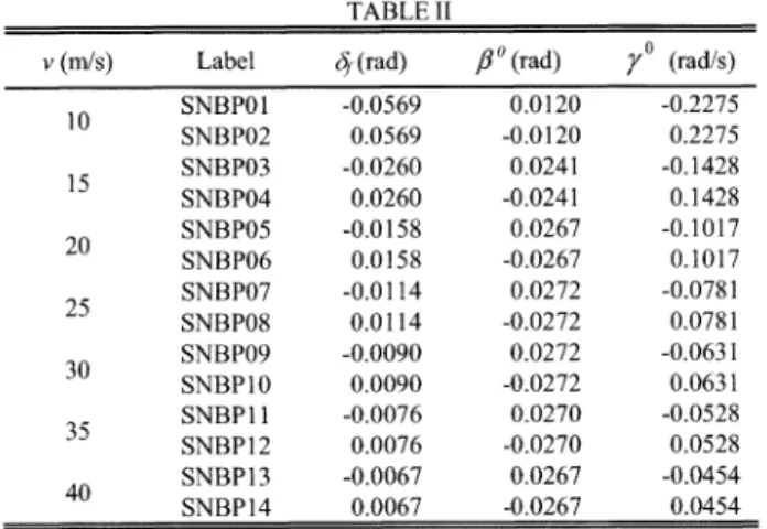
Inthispaper,the computer code AUTO [13] is used to do the numerical analysis, which can calculate system eigenvaluesofJacobianmatrixateachequilibrium pointand determine the corresponding system stability. Bifurcation diagram of system(4)-(5)withrespecttothe variationoft5 is obtained as shown in Fig. 2. Note that, in the bifurcation diagram shown in this paper, the square box denotes the saddle node bifurcationpoint,thesolid-line denotes the stable equilibrium point and the dashed-line denotes unstable equilibrium point, respectively. As shown in Fig. 2, all the system equilibrium points near the origin are found to be asymptoticallystable for differentsettingvalue of thedriving speedv,whichwereboundedbythe saddlenodebifurcation points. Location of those bifurcation points for different setting value of thedrivingspeedv arelisted in TableII. Itis alsoobservedfromFig.2that the systemequilibrium changes stability at the saddle node bifurcation point and the magnitude of

5f

correspondingtothesaddlenodebifurcation becomessmallerasthevelocityvincreases.

TABLE II

v(m/s) Label 4(rad) / 0(rad) y (rad/s)

I10

SNBPO1

-0.0569 0.0120

-0.2275

SNBPO2

0.0569 -0.0120 0.2275 SNBPO3 -0.0260 0.0241 -0.1428 15 SNBPO4 0.0260 -0.0241 0.1428 20 SNBPO5 -0.0158 0.0267 -0.1017

SNBPO6

0.0158 -0.0267 0.1017 SNBPO7 -0.0114 0.0272 -0.0781 25 SNBPO8 0.0114 -0.0272 0.0781 30 SNBPO9 -0.0090 0.0272 -0.0631

SNBP1O

0.0090 -0.0272 0.0631 SNBPI1 -0.0076 0.0270 -0.0528 SNBP12 0.0076 -0.0270 0.0528 SNBP13 -0.0067 0.0267 -0.0454 SNBP14 0.0067 -0.0267 0.0454

To demonstrate the effectivenessofthe

proposed designs

inSectionIV,weconsiderto constructthe linear control laws

forsystem stabilizationatthetwobifurcation

points

SNBPO1 andSNBP13,

respectively.

Detailsare

given

asfollows.

A. ControlDesignfortheEquilibriumPointSNBPO] First,weconsidertodesign state feedback controllers for the low speed driving at v = 10 m/s. To check the

controllability of

SNBPO1,

we have

det[C]

=209.211. 0.

Hence, SNBPO1 is controllable. The next result follows readily from Theorem 1 for system stabilizationdesignatthe pointSNBPO1.

Corollary 2. The saddle node bifurcation point SNBPO1 of system (4)-(5) is asymptotically stabilizable by the linear control law if the feedback gains

ki

and k2 satisfy the following two conditions:

(i) k2 >-0.2838, (32)

(ii) -2.5276-5.9996k2

<ki

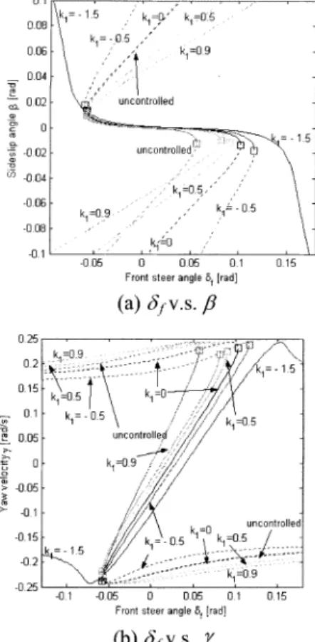
<0.0056+2.9267k2. (33) Asdepicted in Fig. 2, the front-wheel angle

6f

will affect the existence of equilibrium points. In order to seek for a better control gains for system stabilization, let

k,

be treated as another bifurcation parameter. A two-parameter analysis of saddle nodebifurcation isobtained for k2 0.1 as depicted in Fig. 3, which indicate the location of saddle node bifurcation points. The symbol"s"in Fig. 3 denotes the stable operating zone, while "u" denotes the unstable operating zone. It is observed from Fig. 3 that the number of saddle node bifurcation will be different as

k,

varies. In addition to those bifurcation scenarios shown in Fig. 3, there are two more saddle node bifurcation points for 32.8656>

k,

> -0.99 and four saddle node bifurcation points for -1.2605<

k,

<-0.99. Moreover, there is no saddle node bifurcation point for k,<

-1.2605.

Figure 4 presents four saddle node bifurcation points when

k1=

-1.2 and k2= 0.1, and Figure 5 shows the bifurcation diagramwith respect to the differentsettingof

k,

atk2 = 0.1. Theobservations from of Fig. 3 are verified by those shown inFigs. 4 and 5. For k2= 0.1, the equilibrium pointSNBPO1 of system(4)-(5)isasymptoticallystable when -3.1276<

ki

< 0.2982.FromFig. 6, we canobserve the stability ofSNBPO1

atdifferent value of

ki.

We found that SNBPO1 is a stable equilibriumpoint for

k1

=- 1.5, -0.5and 0 whileSNBPO1 is an unstableequilibriumpoint for

k,

= 0.5 and 0.9. Those agree withthe results ofCorollary 2.

B. ControlDesignfor theEquilibriumPoint

SNBPJ3

Next, we construct the stabilization control laws for the system (4)-(5)atthe saddle nodebifurcationpointSNBP13. AsobservedinFig. 2(a),the stableregionof

3f

is very small forv=40 m/s. To check the controllability ofSNBP13,we

havedet[C]= 264.339 . 0 Hence, the linearized model at

the point SNBP13 is controllable. Follow the same control schemeasproposedin Theorem 1,wehave thenextresult. Corollary 3. The saddle node bifurcationpointSNBP13 of system (4)-(5) is asymptotically stabilizable by the linear

control law if the feedback gains

k1

and k2 satisfy the

followingtwoconditions:

(i) k2 >-0.1306, (34)

(ii) -3.2952-23.9914k2 <

kI

<0.0004+1.2481k2. (35) Similarly, let k2 = 0.1. A two-parameter bifurcation diagram of

df

and

k1

isdepictedinFig. 7, which presents the location of saddle node bifurcation points. There are two

-1.1625, there is no saddle node bifurcation point. For -1. 1625<

k,

<-1,there are four saddle node bifurcation points. Figure 8 shows four saddle node bifurcation points at v=40 m/s, k1= -1.1 and k2= 0.1, and Fig. 9 shows bifurcation diagram with respect to the different values of k1 atk2 = 0.1. When

k,

= 1,there is nosaddle node bifurcation point and all equilibriumpoints of system (4)-(5) are unstable. At k2 =

0.1,

the equilibrium point SNBP13 of system (4)-(5) is asymptoticallystable for -5.6943 <

kl<

0.1252. Thestability of system (4)-(5) at SNBP13 for different values of

k,

is shown in Fig. 10. Those agree with the result ofCorollary3.

VI. CONCLUSIONS

In this paper, we focused on the nonlinear study of the second-order model of vehicle's lateral dynamics. The stationarybifurcationphenomenon is predicted and observed inthis system. A direct statefeedback designwasproposed to stabilize the system at the bifurcation point. The two-parameterbifurcation analysiswith respecttothesetting ofcontrol gains were also obtained, which can provide a guide for the selection of the applied control efforts for preventing and/or delaying the occurrence of system instabilities.

REFERENCES

[1] J.Y.Wong,TheoryofGround Vehicles. John Wiley &Sons, Inc., 2001.

[2] J. Ackerman,J.Guldner,W. Sienel,R.Steinhauser, and V. I. Utkin, "Linear and nonlinear controller design for robustautomaticsteering,"

IEEETrans.Contr.Syst.Technol., Vol.3, pp. 132-143, 1995.

[3] H. Peng, and M. Tomizuka, "Vehicle lateral control for highway automation,"Proc. 1990AmericanControl Conference, San Diego,CA, May23-25, 1990.

[4] H. Peng, T.Hessburg,M.Tomizuka, andW.Zhang,"Atheoreticaland

experimental studyonvehiclelateral control,"Proc. 1992 American

ControlConference, Chicago,IL, June24-26,1992.

[5] E. Ono, S. Hosoe, H. D. Tuan, and S.Doi, "Bifurcation in vehicle dynamics and robust front wheel steering control," IEEE Trans.

Control Systems Technology, Vol.6, No. 3, pp.412-420,1998.

[6] L. R. Ray, "Nonlinear stateand tire force estimation for advanced vehiclecontrol,"IEEETrans.ControlSystemsTechnology, Vol.3, No.

1,pp.117-124,1995.

[7] N. Kopell and L. N. Howard, Bifurcations and trajectories joining

criticalpoints, AdvancesinMathematics,Vol. 18,pp.306-358, 1975. [8] E.H.Abed andJ. H. Fu,"Local feedback stabilization andbifurcation

control, II. Stationary bifurcation," System andControlLetters,Vol. 8,

pp.467-473, 1987.

[9] D.-C.Liaw andE. H.Abed,"Stabilization of tethered satellites during station-keeping,"IEEETrans. AutomaticControl, Vol.35, No. 11,pp.

1186-1196,1990.

[10] D.-C. Liaw and E. H. Abed, "Active control ofcompressor stall

inception:abifurcation-theoretic approach,"Automatica, Vol. 32, No. 1,pp. 109-115, 1996.

[11] D.-C. Liaw andC.-C. Song, "Analysis oflongitudinalflightdynamics:

abifurcation-theoretic approach," Journal of Guidance, Control,and

Dynamics, Vol.24, No.1,pp. 109-116,2001..

[12] D.-C. Liaw, H.-H. Chiang, and T.-T. Lee, "Abifurcation study of

vehicle's steering dynamics," Proc. IEEE 2005Intelligent Vehicles

Symposium,LasVegas,Nevada,USA, June 6-8, 2005, pp.388-393.

[13] E.J.Doedel,AUTO: Aprogramfortheautomaticbifurcationanalysis

of autonomous systems. Congressus Numerantium, Vol. 30, pp.

265-284, 1981. 0° 5 ' .0 " ' 004 0.02 [V=40m/s 0.01 0 v=lOm :0-01 CO-0.02 v=20ms i -003 -0.04 -0.06 -0.04 -0.02 0 0.02 0.04 0.06 Front steerangle8,[radl

(a)

1f

v.s./1 0.25 0.2 --vOm- s -010 vo16m/s --- ---0.1 --- ---¢- - --- 01--0.1 ---,-. 0.15 -0.2 .---dis| -uzz -0.1 -0.05 0 0.05 0.1

Front steerangle0,[radl

(b)1fv.s.

7

Fig. 2.Bifurcation diagram withrespect to different v.

-0.1 -0.05 0 0.05 01 0.15 Front steerangleO,[rad]

Fig.3.Two-parameterbifurcationdiagram for

5f

v.s.

ki

when v=10m/sand k2=

0.1

. 015 0.1 0.06 c:2 I c 0 -0.06 -0 1 -015 -012 00 0I 0 1 00 0 -O1. -0.0 Q 0.05 0.1 0.15 0.2 Front steerangle [rad]

Fig. 4. Bifurcation diagramwhen v=10 m/s,ki=-1.2 and k2

0.1. =o201 uncontrolted 1~~ ~ ~~~~0 unIont d =01 uncont ncntrolle -1 I'll 0.2, -1 5

L-0.08 0.06 004 005 -008 -0.1 -0.05 0 0.05 0.1 Frontsteerangle0,Irad]

(a)

1fv.s.

, 0.15 0.25 \1 kl -O 1 -''' 0.15 -0.21 00 0 1 r~~~~~~~~-incontrolled 0 05

ao

C: 01 -0 15 -02 -0.25--006 -0.04 -0.02 0 002 .004 0.0 0.00 0.1 Frontsteerangle0,[rad]

Fig. 8. Bifurcation diagram when v=40 m/s,

ki

-1.1 and

k2-0.1. 0.06 0.04 002 0--0.02 -004 -0.1 -0.05 0 005 01 0.15

Frontsteer angle5,[rad]

(b) 3fv.s. 7

Fig. 5. Bifurcationdiagram withrespect todifferentk0 when

v=10 m/s andk2=0.1. 0.017 to1= 0~5 0.016 1 0 015 05 0.014 1.5 0.013 =- 1 0. ~0.012-r 011ouncontod 1 0.011 -~5'0. 0.01 0000~~ ~~~~~~k= -0.06 -0.059 -0.058 -0.057 -0.056 -0.055

Frontsteerangle0,[radl

Fig.6. Zoom inonFig. 5(a)nearSNBPO1.

-2 01

3t -O. c

-004 -0.02 0 002 Front steerangle5,[rad]

(a) jfv.s.

0.04 105

(b) 3/vS. 7

Fig.9. Bifurcation diagram withrespecttodifferent k1 when

v=40m/s andk2= 0.1.

Fig.7.Two-parameterbifurcationdiagramfor 3fv.s.k1 when

v=40 m/s andk2 =0.1. Fig. 10.Zoom inonFig.9(a)nearSNBP 13.

k. -,.5 k 05 9

\,

'26-4 uncontrolled uncontrolledd =0\ k =09 ' ~~ki--0.5 11S kt Q°5 k to1 05 to 1=15 /k - ,F2 uoncontrolled /1?~~~~~~~~~~. kt=05 to0os 1 . -o f UIlk ...l U. UU -U.UbO _ c