TRADE AND THE LOCATION OF INDUSTRIES
IN THE OECD AND EUROPEAN UNION
1by
Michael Storper2, Yun-chung Chen3,
and Fernando De Paolis4
March, 2001
Accepted for publication in The Journal of Economic Geography
Abstract
Trade and location theory identifies forces that could lead to locational dispersion (comparative advantage) or locational concentration (scale economies) in the face of globalizing markets, each with different consequences for specialization and the adjustment costs associated with integration. However, these forces can play
themselves out in very complex ways if locational change principally affects intermediate production.
Moreover, effects of history may be important, if locational patterns which exist prior to integration reflect either strong external economies or, as we argue, strong institutionalized capacities to respond to more open markets. This could especially be the case in the context of Europe, whose territories are generally less specialized than the States of the USA. To see how these different effects are operating today, empirical measurement is
1
An earlier version of this paper was presented to the DRUID (Danish Research Unit on Industrial Dynamics) 1999 Summer Conference, Rebild, Denmark, and to the London School of Economics. Thanks are due to participants in that meeting for their helpful comments. We also wish to thank the Academic Senate of the University of California, Los Angeles Division, for financial assistance, as well as the LATTS (Research Center on Territories, Technologies and Societies) at the Ecole Nationale des Ponts et Chaussées in France, for logistical support, and to the OECD in Paris for supplying data. We would also like to acknowledge the generous intellectual assistance of Professor Chandler Stolp of the LBJ School of Public Affairs, University of Texas at Austin, and to Dr. Andres-Rodríguez-Pose and two anonymous referees for their insightful critiques of an earlier version.
2
Professor, School of Public Policy & Social Research, UCLA (Los Angeles) and Professor, Social and Human Sciences, Université de Paris/Marne-la-Vallée (France): [email protected]
3
Doctoral candidate, UCLA (Los Angeles): [email protected] 4
required. Using a data set which allows changes in locational distribution of manufacturing industries in the OECD to be measured, we show that Europe does not seem to be "Americanizing" its economic geography. Many sectors are actually spreading out in Europe, implying that the effects of history have remained strong up to this point. Specialization increases are weak in most European economies as well. The OECD has a more complex picture of spread and concentration. Some of the implications for further research on agglomeration, intra-industry trade and integration are brought out in the conclusion.
JEL classifications: F14, F20, R14.
Keywords: trade, industrial location, intra-industry trade, specialization, economic geography, agglomeration,
integration, globalization, European Union.
____________________________________________________________________________
I. THEORETICAL PERSPECTIVES ON GLOBALIZATION AND LOCATION
The globalization of production and integration of markets have many possible effects on the location of
economic activity. Classical Ricardian trade theory, if applied directly to a world of decreasing trade barriers and
transportation/transactions costs, suggests that comparative advantage effects will be freed up to play themselves
out on a wider spatial scale, leading to rearrangement of activities on the landscape. The economies of places
will generally become more specialized, clearer expressions of their globally-redefined comparative
advantages (Ricardo, 1963;Balassa, 1963). The trade and location theories of the New International
Economics/New Economic Geography lead to a similar overall prediction, but for different reasons. Scale
economies -- internal and external, and various combinations of both -- which could not be fully realized with
specialization of regional and national economies, and inter-industry trade among them (Helpman and Krugman,
1985; Krugman, 1991; Fujita, Krugman, and Venables, 1999). The two dynamics can combine, moreover, to
heighten each other’s effects.
These theories do not only concern inter-industry patterns of specialization and trade. Given that complex
intermediate input-output systems characterize most of modern productive activity, comparative advantage or
scale effects should encourage the international reorganization of commodity chains (filières), resulting in
growing intra-industry trade. Thus, much of contemporary trade theory and international economics predicts
that globalization will lead to more intra-industry specialization of national economies. The NIE actually makes
two very different predictions about possible overall effects of trade opening on the degree of specialization of
regional economies. When referring to scale and comparative advantage effects on inter-industry trade, authors
such as Krugman (1991) predict that the member countries of the European Union (EU), as they pursue their
project of integration, will become more similar to regions of the United States, which are much more
sectorally-specialized than territories of similar extent in Europe. This is because agglomeration effects will play
themselves out in a context of larger market areas. By contrast, when they refer to integration through heightened
intra-industry trade, they envision a Europe where countries with similar development levels (i.e. Northern
Europe) will become more specialized in particular intermediate outputs in the same branch of production
(Krugman and Venables, 1996). This will have the overall effect of preserving a dispersed locational pattern
and avoiding "Americanization" of Europe's industrial geography (Commissariat Général du Plan, 1999). As we
in determining how location patterns respond to integration.
One of the most complex issues is the spatial scale at which specialization and agglomeration effects might
operate. If agglomeration is principally relevant at the regional or metropolitan scale, then it could well be
possible that nations could retain roughly similar shares of world trade in a given industry, while simultaneously
experiencing significant locational concentration within the national territory. Heightened locational
unevenness would only show up, in this case, as a subnational effect, not necessarily as a change in a country's
position in world trade, or in an industry's degree of locational concentration. The problem is that data are not
available to carry out consistent comparative international measures of trade and location at the subnational
regional scale.
Another difficulty in making sense of trade is that the term "intra-industry trade" is not very precise.
When a French car firm imports its motors from Germany, and assembles cars in France, while exporting
transmissions to a German car firm, this is considered to be intra-industry trade.5 Or, a French car firm might
import motors for some of its models from Germany, while other German firms might import their motors from
French car firms. Trade could also be one-way, as when important computer components made only in the
United States are imported into other countries (whether through intra-firm or inter-firm trade), and assembled
into electronic goods. In other cases, a country will export components or partially-finished goods to another
country, and the final product will subsequently be sold in the original home country. These are all examples
known as international "production sharing." Intra-industry trade also covers cases of cross-hauling, i.e.
bilateral trade in similar final outputs. This has different causes and may have different developmental
consequences from international production sharing.
Moreover, regions or nations can specialize in products whose factor contents differ substantially.
When the average quality of the outputs is higher in one country or region than another, the value of their factor
services differs. Such vertical specialization could have big impacts on overall location patterns for a given
industry. Its potential number of locations is a function of the length of its quality ladders, because different
factor contents can create alternative agglomeration patterns from those found in industries where trade is
horizontal. This could be true for both final and intermediate outputs, with the two effects combining
(Grossman and Helpman, 1991).
Thus, world market integration brings together functionally similar products from formerly divided
markets, which correspond to different quality-based preference rankings and consumer budgeting; hence, when
the German and French car industries come into open contact with each other, the Germans are more specialized
in better quality and more expensive cars than the French, and market integration tends to expand the markets for
their vertically-differentiated final outputs, maintaining their differences rather than effacing them (cf.
Bergstrand, 1990).
Thus, the term "intra-industry trade" could refer to four different organizational and locational
phenomena: cross-hauling of functionally-similar final outputs (vertical and horizontal), and trade between
countries involving different intermediate stages of a single filière or commodity chain, also vertical and
horizontal. In addition, certain types of inter-industry trade (based on agglomeration economies) can also be
vertically differentiated. The way that most research on trade is carried out (using sectoral nomenclatures),
these are difficult to disentangle (Fontagné et al, 1997).
Though there is a huge theoretical literature, and there is considerable empirical literature on trade alone,
there is very little empirical literature on the relationships between trade and location together, and even less
which links them to patterns of specialization and national/regional income effects. There is general agreement
that intra-industry trade is rising in the vast majority of sectors. Moreover, the northern members of the
European Union have a higher average level of quality in the products they export to the southern members than
they import from the latter (Fontagné et al, 1997). National per capita incomes have tended to converge in
Europe over the past several decades, though there remain much bigger gaps between the poorer and richer
countries of the EU than between the states in the USA. At the subnational level, the evidence suggests
continuing or even growing divergence between core and peripheral regions (Rodriguez-Pose, 1998). In France,
for example, while overall incomes have tended to converge between regions, gross output per habitant has
tended to diverge between the major metropolitan regions and the rest of the country, with the difference
between the two measures due to increasing volumes of transfer payments (Davezies, 2000). While there is
little systematic evidence on changes in locational patterns at the international scale, some studies suggest that
Midelfahrt-Narvik et al, 2000). Paralleling the increasing divergence between regions, some authors argue that
the metropolitan share of national output in European countries is increasing due to more uneven subnational
distributions of industries (Veltz, 1996; Thisse, 1998).
The analysis of relationships between trade, location and specialization presents considerable
methodological challenges. Location patterns and specialization are measured via output or employment data.
Data sets, for a consistent set of industry codes over time and for a large set of countries, at the three-digit or
more6 level of resolution, generally contain either trade or output (the proxy for location) information, but not
both. So, most empirical research contents itself to analyze either trade or location, but not their
interrelationships. In what follows, we present the results of our investigation of the degree of international
locational concentration, the level of intra-industry trade, and national specialization for a set of 26 three-digit
manufacturing industries. This was carried out at the level of the OECD (Organisation for Economic
Cooperation and Development, consisting of 24 countries in our data set) as a whole, and then for 13 of the 15
EU countries, which are tied together by even higher levels of trade than the OECD as a whole. This data set
does not allow analysis of location and specialization at the subnational regional level, nor does it shed light on
vertical specialization and its possible effects on incomes. It is therefore a first step in investigating the field of
interrelations identified above; the results reported here allow us to formulate more advanced hypotheses about
II. DATA AND METHODS
The OECD-STAN (Structural analysis Database) 7 is one of the few data bases to contain information
on both trade and output for a consistently-defined set of two-, three-, and four-digit ISIC manufacturing sectors,
for the OECD countries, who account for most of the trade and output in the world economy. The data are also
available over time, annually for the period 1970 to 1994, during which trade levels and the share of trade in
output of 25 out of our 26 industries increased, with a strong increase in 23 of them.8
TABLE 1: OECD, Ratio of trade to output 1970-1994
Since the data are reported by the OECD in national currency units, they had to be converted into a
common unit and indexed to constant value. In addition to converting them all to 1997 dollars, using the U.S.
GDP deflator Index,9 we first converted the national data into Purchasing Power Parity units, using the OECD’s
6
Indeed, this sort of analysis ideally would require data at the four- or even five-digit levels, so that patterns of production could be compared at the level of narrowly-defined product groups.
7
The STAN (structural analysis database) was created to fill the gap between the detailed data collected through industrial surveys (such as those found in the OECD's ISIS database) which have limited international comparability, and national accounts data which are more internationally comparable but only available at fairly aggregate levels. Through the use of established estimation techniques, the OECD Secretariat has created a database that is compatible with national accounts for 22 countries. It covers 49 ISIC-defined manufacturing industries for six variables with annual data from 1970’. Cited from http://www.oecd.org/dsti/sti/stat-ana/index.htm. In this paper, we only use two of the variables, i.e. exports and imports, and value of production. The other variables are: value added, gross fixed capital formation, number engaged and labor
compensation. 8
Our data set does not include service industries. However, since most of the conceptual apparatus of trade and location theory, especially with regard to economies of scale, was developed with manufacturing in mind, the limitation of the exercise to manufacturing helps us target explanations of location in light of increasing trade. Obviously, future work will have to extend to services. Another limitation of the data is that they concern only the OECD countries. Though this gives us the lion’s share of world trade, it means that in those manufacturing sectors with high levels of import or export to
non-PPP index.10 This is the appropriate strategy in using the data to analyze location. Production data reflect the
market value of output, not physical quantities. Production values can be distorted by exchange rate fluctuations.
Some distortion remains, since there are productivity differences between countries. But because we are
analysing a sample of highly developed countries with roughly similar total factor productivity levels and limited
variations in sectoral productivity,11 the correction from converting to PPP should be broadly correct.
We then carried out two tests on the output data, for each sector over time. In order to detect changes
in the international location of an industry, we employ a measure of the sector's locational evenness or unevenness, the Herfindahl equivalent index (HE),
where Y is the value of output, i stands for the sector, j for the country, and R for regions.
Where R=EU, it refers to the 13 countries in the European Union and where R=OECD it is 24 OECD member
countries. The higher the value of the index, the lower the industry's international spatial concentration. This is
because the HE corresponds to the number of standardized territorial units (in this case countries of the OECD)
that would be necessary to attain the observed total share of world production.
We then measured the level of intra-industry trade (IIT) with the Grubel-Lloyd index (Grubel and
10
Data obtained form 1998 edition of National Accounts Volume 1: Main Aggregates 1960-1996, page 174-175. Paris: OECD, Division of Science, Technology and Industry (DSTI).
11
If underlying productivity levels were greatly different, then PPPs would be distorting. However, in most industrial sectors, the OECD countries fluctuate within a band of 85-105% of US productivity.
∑
=
j iR ij R iY
Y
HE
2 , ,1
(
)
Lloyd, 1975):12
where: 0<GL<1, i stands for sector, j for country, X for exports and M for imports. To account for
change, year-to-year fluctuations had to be eliminated, so t1 was defined as the 1970-74 average of yearly means
for the two indices, and t2 as the 1990-94 average of yearly means, for each country and sector studied (Table
2).13 The GL index is generally calculated on the basis of bilateral intra-industry exchanges, between a given
country to a given trading partner and within a given sector. We adopted a slightly different approach, in that we
calculated average GL indices for a given sector with respect to a group of countries (R), either 13 EU member
countries or 24 OECD member countries.14
The goal of the analysis is to determine how changes in locational distribution of an industry are related
to changes in intra-industry trade, as reflected in the co-evolution of the GL and HE indices for each industry.
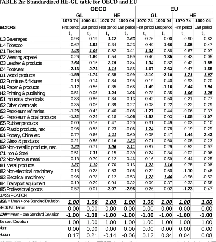
Since they have different scales to begin with, and since each index has a different mean in t1 and t2, change
was measured as departure from the respective mean, in standard deviations, i.e. z-scores(Table 2A). This
12
The GL index, as is well known, cannot distinguish between vertical (quality differentiated) and horizontal (factor-neutral differentiated) trade in final outputs, nor between cross-hauling of final outputs and intra-industry trade due to international divisions of labor within an industry (production sharing). Our HE index cannot distinguish between concentration due to many units as opposed to a big unit, as is possible with the alternative Ellison-Glaeser index. Our data set does not permit these distinctions, but they will be taken into account in the discussion in the final section of the paper.
13
We are primarily interested in change over the entire period examined here, where trade underwent a very considerable increase, and therefore we do not analyze year-to-year fluctuations within the period.
M
X
M
X
ij ij ij ij iGL
+
−
−
=
1
|
|
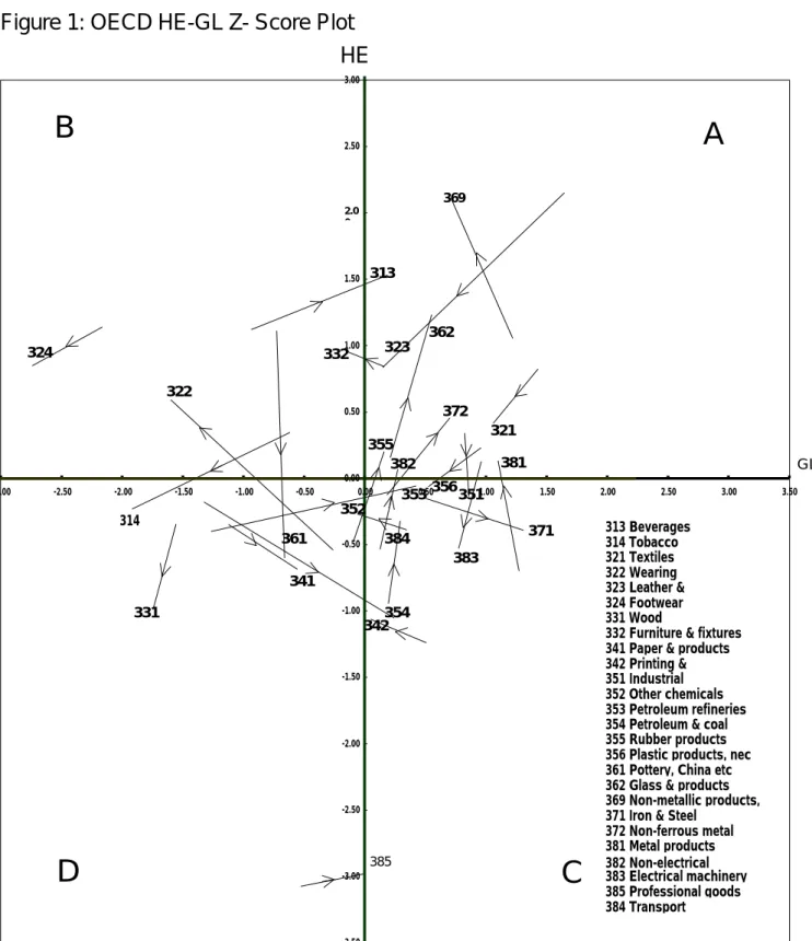
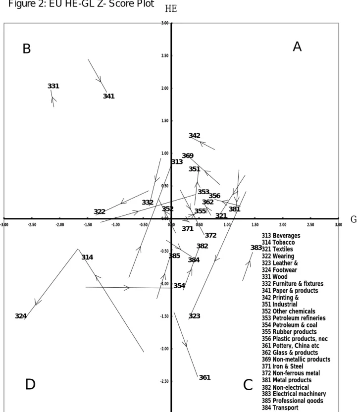
effectively removes the influence of absolute values. Each sector's z-score was then plotted according to its
positions in t1 and t2, with HE on the vertical axis and GL on the horizontal, as shown in Figure 1 for the OECD
and Figure 2 for the EU.
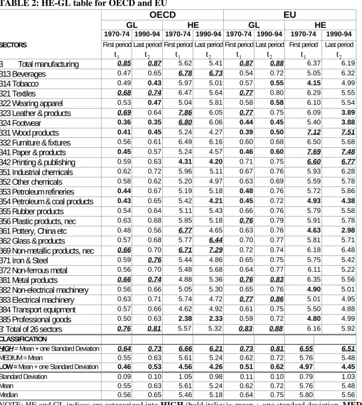
Table 2: HE/GL table for OECD and EU
Table 2A: Standardized HE/GL table for OECD and EU
Figure 1: OECD HE-GL z-score plot
Figure 2: EU HE-GL z-score plot
There is a potential problem with an analysis which classifies sectors into quadrants defined by the
means. Though means are the best representation of a set of values, the values of the means do not necessarily
correspond to any real threshholds of difference in the concrete reality of industrial sectors. A sector could
cross a mean with little overall change in position, whereas another sector might remain within a quadrant by
changing position considerably within it. To provide a check on this possibility, we therefore carried out a
second analysis of the HE-GL relationship, this time grouping sectors exclusively according to the direction of
change in the two indices, and ignoring absolute position. To do this, we group the industries that exhibit the
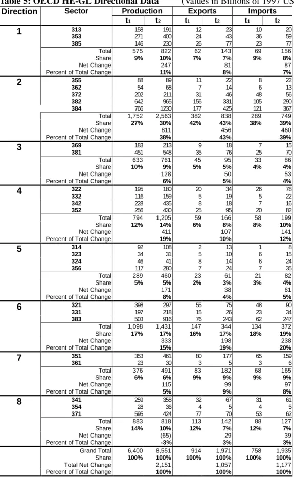
same direction of change from t1 to t2.15 Tables 5 and 6 show the results of this analysis. The purpose of this
directional analysis is to understand the tendency of HE and GL over time, regardless of their original positions.
The directional analysis is the most relevant to understanding change.
Table 3: OECD HE-GL Positional Data
15
Thus, direction 1 refers to industries that move toward the northeast (decreasing locational concentration and increasing intra-industry trade); direction 2 is northeastward (decreasing concentration and decreasing IIT); direction 3 is
southwesterly (increasing concentration and decreasing IIT); and direction 4 is toward the southeast (increasing concentration and increasing IIT).
Table 4: EU HE-GL Positional Data
Table 5: OECD HE-GL Directional Data
Table 6: EU HE-GL Directional Data
As we shall see, the two methods indicate similar overall tendencies, albeit with somewhat different
magnitudes. Thus, we can be confident that the overall story about change in location and its relationship to
levels of intra-industry trade that we are about to tell is not merely an artifice of our use of means as cutoff
points between categories.
III. THE MAIN TENDENCIES
Before examining the complex relationships between intra-industry trade and locational patterns, we
first checked for the tendencies in each of our main indices. Regressions across time – which measure the
temporal strength and directional consistency of the evolution of the index -- were run, using as dependent
variables the Grubel-Lloyd (GL) or Herfindahl equivalent coefficients(HE) across all years, on a year-by-year
index, and holding industry size constant with dummy variables. The results for the GL and HE regressions are
markedly different.
Intra-industry trade is increasing with remarkable constancy, across nearly all industries, and in both the
EU and the OECD. For the OECD, the overall parameters on both regressions are positive and strongly
significant for 22 out of 26 sectors (sectoral data are not reported in the table). For the EU, the parameters are
greater. This is probably because the dismantling of trade barriers and progress of integration has been even
faster within Europe than within the OECD overall in the period under examination. These regression results
are supported by the box diagram for the GL coefficients in Figures 3 and 4. There is more dispersion of the GL
ratios in the OECD than in the EU, but in both, there are significant differences between industries, possibly
having to do with durable inter-industry differences, possibly to different phases of their development.
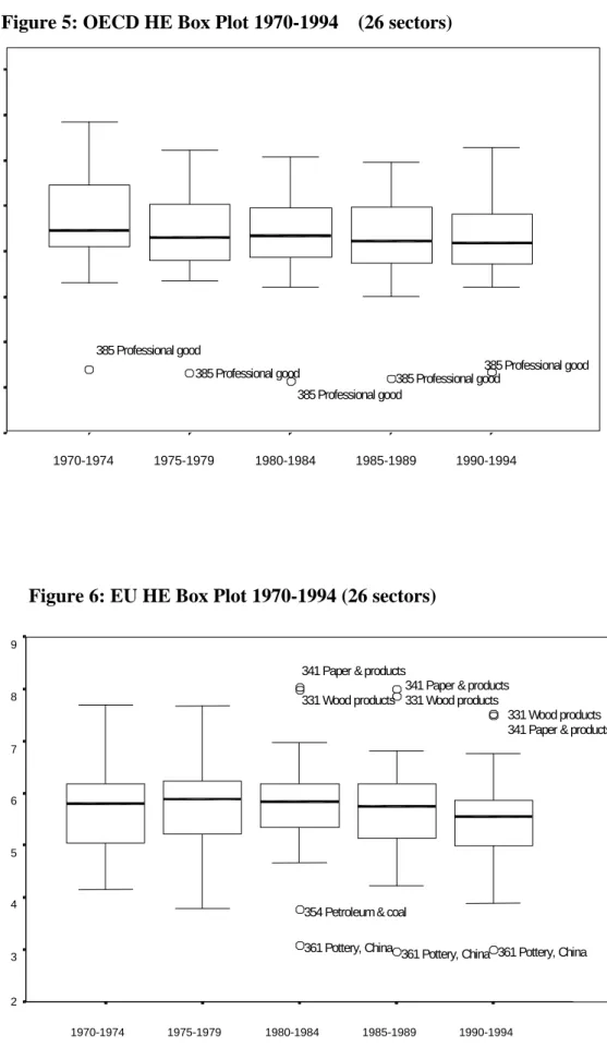
Figure 3: OECD GL Box Plot, 1970-1994 Figure 4: EU GL Box Plot, 1970-1994
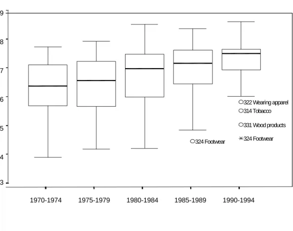
Figure 5: OECD Herfindahl Equivalent Index (HE) box plot 1970-1994 Figure 6: EU Herfindahl Equivalent Index (HE) box plot 1970-1994
The story is quite different when it comes to the locational tendencies of industries. For the OECD, the
time series regressions for the HE have parameters that are both weakly negative. In the second test, moreover,
the result is not robust (see t-statistic), and the industry-by-industry results are extremely heterogeneous. For the
European Union, the first parameter is weakly negative but robust, while the second is weakly positive and not
robust, again with great variability from sector to sector. This lack of clear tendency can be seen in the box
diagram. These results are consistent with Midelfahrt-Narvik, Overman, Redding and Venables (2000), who
--using the same data set -- found mixed evidence on average sectoral locational concentration in the EU, and
The heart of our investigation consists in combining the two indices and then tracking the changes in
position over time for each of the 26 three-digit sectors. As noted in the previous section, this was done in two
ways, via analysis of position (Figures 1 and 2; Tables 3 and 4) and through an analysis of direction of change
(Tables 5 and 6). In the northeast quadrant (A), we find high levels of IIT and low levels of locational
concentration (high HE, high GL); in the southeast quadrant (C),high levels of IIT and high levels of locational
concentration (low HE, high GL); in the northwest quadrant (B), there are low levels of IIT and low levels of
geographical concentration (low GL and high HE); and finally in the southwest quadrant (D), there are low
levels of IIT and high levels of geographical concentration (low GL and low HE). Industries that fall close to
the means must also be interpreted with considerable caution.
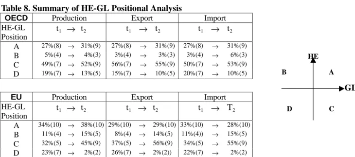
Table 8. Summary of HE-GL Positional Analysis
Table 9. Summary of HE-GL Directional Analysis
Table 10: Shares of Total Change in HE-GL Directional Analysis
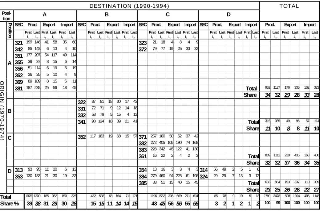
The analysis of position is summarized in Table 8 (OECD Origins t1 + destinations t2). The values in
the columns indicate the shares of production, imports and exports for the sectors found in each quadrant in the
first or second period. For example, in quadrant A for the OECD, the share of production decreases from 31%
to 27%, while the same quadrant for the EU shows an increase from 34% to 38%. This indicates that the shares
4% in both the OECD and the EU countries.16
The result for the OECD is quite clear: the growing sectors are going predominantly toward
destination C (52%), with A remaining very important (31%), while the B and D destinations are small and B
is nearly insignificant. By reading the changes in row totals, we find out that changes in origins were not so
important as destinations: production shares did not undergo big changes by origins, presumably because
industries underwent considerable restructuring during this period, causing them to move from one destination
category to another.
The actual shifts in shares of production, exports and imports for the industries in each quadrant for t1
and t2, for the OECD, are rather modest. For output, 12 sectors which start out with low locational
concentration (in A and B quadrants) show an increase in their share of production from 32% to 35%, while the
14 sectors initially with high locational concentration (in quadrants C and D), experience a slight decline in their
share of production, from 68% to 65%. There is growth in the share of sectors with IIT above the GL mean, from
76% to 83% (production shares of A+C). In general, category C accounts for more than half of total production,
exports, and imports. This first glance at the evidence thus suggests a picture which does not conform to the
predictions of standard theory; in a period of strongly growing overall trade, sectoral locational concentration
appears not to have increased across the board. On the contrary, the aggregate effect actually inclines toward
more output in locationally spread sectors (a 3% increase), with less output in concentrated industries (3%
decrease).
16
The EU countries are following a pathway which resembles that of the OECD in its broadest outlines,
but there are several important differences as well. The sectors with above-mean IIT increase their share of
production from 66% to 83% , almost exactly as in the OECD. The shares of A and B actually increase from
45% to 53%, for 14 and 15 sectors, respectively, an 8% increse for the EU as compared to 3% for the OECD.
The shares of more concentrated sectors (quadrants C and D) decrease from 55% to 47%, i.e. 8% as opposed to
just 3% for the OECD. This implies that the widelyheld idea that the EU is simply less far down the pathway
-- toward locational concentration and growing intermediate trade ---- traced out by the OECD, is not correct, since
in the EU there was actually an important increase in the share of industries with HE above the mean, and
greater decrease in the more concentrated sectors (HE below the mean). In absolute terms in 1990-94, , the EU
has a much larger share of less concentrated sectors (A+B) than the OECD (53% versus 35%). More importantly,
as indicated in Tables 3 and 4, inter-quadrant mobility is higher for the OECD than the EU, although both
show increases in quadrants A and C. Thus, sectoral locational patterns in the EU are more stable than in the
OECD, with less inter-quadrant movement of sectors. Most of the EU sectors end up in the same quadrant from
which they originated, and this is especially pronounced for quadrant A of the EU. For the OECD, the
origins are quite diverse, and the destinations more concentrated. Put another way, the distribution of sectors
is more concentrated on the diagonals for Table 4 (EU) than Table 3(OECD).
As was noted, we wanted to be sure that the four categories employed above are not mere statistical
second analysis, where we analyzed the direction of change of each industry, irrespective of its position. The pie
chart next to Table 9 shows graphically the directions of change whose realization would correspond to the four
destination categories used in Figures 1 and 2. Thus, directions of change 1+2 move industries toward
destination A, 3+4 in B, 5+6 in D, and 7 +8 in C. Since these are tendencies rather than destinations, the
sectors in each category do not necessarily correspond to those in the destination categories analyzed above.17
Table 9 summarizes the direction data. Table 10 then shows the shares of change accounted for by industries
going in each of the measured directions.18 The overall sense of the two analyses is very similar.
Both the OECD and EU show tendencies toward more locational spread, and both manifest strong
increases in IIT. The share of less concentrated sectors (sum of directional categories 1 and 2) grew for both the
OECD (58% to 63%) and the EU (53% to 59%). On the contrary, the share of concentrated sectors (sum of
directions 3 and 4) decreased from 43% to 39% in the OECD and 48% to 41% for the EU. However, there are
important differences between the EU and the OECD as a whole. Table 10 shows that the share of total change
accounted for by sectors moving in the direction of greater production spread is slightly higher for Europe (81%)
than the OECD (74%). Moreover, the EU share of total change in IIT grows faster than OECD, 67% versus
53%. This shows that despite more rapid growth in IIT, the EU does not show a higher degree of locational
concentration. This finding further illustrates the tendency of the EU to have a more dispersed international
locational pattern than the OECD, at the same level of IIT development. Though our results end in 1994, this
17
Since these are directions of movement rather than positions, the sectors in each category in the two analyses do not necessarily correspond .
finding is consistent with Midelfahrt-Narvik et al (2000), who analyzed the same data set through 1997.
In summary, three preliminary conclusions can be drawn about current trends in spatial development in the
face of rapidly increasing trade. Across the board, intra-industry trade is rising as a proportion of total trade. In
the OECD, there is a mix between locational concentration and spread, in that the levels of concentration are
greater but the direction of change is for more dispersion. By contrast, in the European Union locational
concentration levels are weaker on the whole, and the intersectoral variation in such tendencies is greater than in
the OECD (Table 7, Figures 3-6). Notably, it appears that
more sectors are either not concentrating or are spreading out in the EU than in the OECD as a whole. The
differences between the OECD and EU probably reflect the greater barriers to trade that still exist between the
three principal zones of the OECD, the EU, North America, and Japan, than within them.
As noted, changes in the degree of international dispersion or concentration of sectors should be connected
to changes in the overall level of specialization of national economies. Bringing them together in a single
model is not possible, but we can trace changes in output specialization. This is done via the Revealed
Comparative Advantage Index (Balassa, 1965), which is expressed as follows:
∑ ∑∑
∑
=
j i j ij ij i ij ij ijX
X
X
RCA
X
/
/
where i represents sector, and j stands for country.
The RCA index contains a comparison of national export structure(the numerator) with the OECD export structure (the denominator). When the RCA equals 1 for a given sector in a given country, the percentage share of that sector is identical with the OECD average. Where RCA is above 1 the country is said to be specialised in that sector and where RCA is less than unity, the country is not specialized in it. Since the RCA is bounded by zero and infinity, it is unwieldy. Therefore, we converted it to a symmetrical index (centered on zero), i.e. (RCA-1)/(RCA+1). The resulting measure ranges from –1 to +1 and resembles a location quotient. The measure is labelled “Revealed Symmetric Comparative Advantage” (RSCA).
In order to test whether overall country specializations are composed of the same sectors or not, and
whether overall increases in specialization are due to reinforced specialization in the same sectors or in different
sectors, we employed a method used by Cantwell (1989) and Laursen (1998). Stability (and specialisation
trends) is tested by means of the following OLS regression equation (country by country):
The idea behind the regression is that if $=1 and " is statistically indistinguishable from zero, this
corresponds to an unchanged pattern from t1 to t2. By contrast, if $>1 the country tends to become more
specialised in sectors where it is already specialised, and less specialised where its initial sectoral specialization
is low; i.e. the existing sectoral pattern of specialization is strengthened. $ >1 is termed $-specialisation.
Similarly, 0<$<1 can be termed $-de-specialisation, i.e., on average sectors with initial low RSCAs increase
over time while sectors with initial high RSCAs decrease their values. In Figures 7 and 8, this specialization is
shown in the northeast quadrant and labelled "same sectors," whereas de-specialization is found in the southwest
ε
β
α
i i ij ijijt RSCAt
and northwest quadrants and labelled "different sectors."
Figure 7: OECD RSCA Specialization Graph
Figure 8: EU RSCA Specialization Graph
However $>1 is not only way an increase in overall national specialisation can be captured (Cantwell, 1989;
Laursen 1998). Following Hart(1976), it can be shown via the following f-test of homogeneity at t1 and t2 that
Thus,
If $>R (equivalent to an increase in dispersion), the degree of specialization has increased, whereas if $<R
(equivalent to a decrease in dispersion), the degree of specialization can be said to have decreased.
There is one impossible case in Figures 7 and 8, where $>1<R; an economy cannot become more specialized in
the same sectors but less specialized in general. So, there are three possible combinations of the two types of
specialization.
For the OECD, two results stand out. First, most countries are in the northwest quadrant, but not very
far within it. They are shedding certain sectors in the context of globalization, an effect of integration predicted
2 2 2 2
/
/
1 2 i i t i t iσ
β
R
σ
=
|
|
/
|
|
/
1 2 i i t i t iσ
β
R
σ
=
changed to a significant degree (UK, Spain, Japan). Japan has offshored much routine production to surrounding
Asian countries due to its rapidly rising labor costs, while Spain's economy has been transformed by its recent
integration into the EU, with important effects of inward FDI. In the EU case, the UK and Spain seem, again, to
be experiencing changes in the sectors in which they specialize, while the Netherlands and Germany are
becoming somewhat more specialized in their pre-existing areas of strength. There are very few countries
which are well away from the two medians in the graph; most countries’ changes in position are minor, as shown
by their presence within the central zone of the Figures 7 and 8. This is quite consistent with what we have
seen about industries' locational behavior. Since national levels of overall specialization are the result of very
heterogeneous industry-by-industry tendencies, we would expect to see such average levels of specialization
change little and quite gradually.
IV. SOME POSSIBLE EXPLANATIONS
Location and Trade Patterns
Figure 9: Stylized Scenarios of Location and Intra-Industry Trade
Ultimately, to explain concrete patterns of location and trade, we would need to be able to link industry
characteristics (such as scale, market structure, factor mix etc) to industrial organization (size and structure of
units, division of labor, etc), and then to locational structure (linkages, spatial transactions costs, agglomeration
moment, however, there is widespread agreement that it is extremely difficult, if not impossible, to explain
locational concentration of industries according to industry characteristics: most attempts to do so are
inconclusive (Brulhart and Torstensson, 1996; Amiti, 1999). Moreover, though theory has a few things to say
about how industry characteristics might affect location patterns, different characteristics push in different
directions, and there is as yet no unified theory on the relationships that would allow specification of an
empirical model. For the moment, we must be more modest in our ambitions. One way to begin is to carry out
a thought experiment about the organizational and linkage structures which correspond to the observed levels of
locational concentration and intra-industry trade, as is depicted in Figure 9.
Cases B and D are relatively straightforward. In B, the combination of low locational concentration
and low intra-industry trade implies that most trade will be in final outputs and that it will be highly
asymmetrical (with exporters and importers not overlapping much), and that there will be a high level of
self-supply without international trade. The development of local input structures could come about for different
reasons, however. In the EU printing and publishing industry (342) for example, it is because of the local
demand structure; whereas in the glassware, furniture, wood products, and paper industries (362, 332, 331, 341),
it is probably because location follows natural resources. The wearing apparel industry (322) for the OECD is,
somewhat surprisingly, found in this group, and we surmise that this reflects the progressive development of
local input structures in countries receiving foreign direct investment, and thus the general expansion of possible
In D, a higher degree of locational concentration could in principle come about for many reasons: big
plants, a high level of agglomeration of the input-output chain (proximity relations between firms in a more
fragmented division of labor), or a selective comparative-advantage based locational process. They would
lead to final output trade and to major asymmetries between exports and imports, and hence to the statistic of
low intra-industry trade. The industries found in this group by the direction-of-change analysis19 are mostly
labor-intensive, nondurables industries. The decline in intra-industry trade is most likely explained by the
increasing adequacy of local supply chains. But why is overall locational concentration rising, especially since
these are industries with considerable potential for product variety and hence for the existence of many locations?
The case study literature often emphasizes the "high end" versions of these industries, such as the famous cases
of Italian industrial districts, which are based on highly specialized local resources and relationships (Storper and
Salais, 1997). But locational concentration at a world scale could also be due or to comparative advantage in
location of mass production of standardized versions of products. This would be concretely manifested in
relocation of these industries to low-wage labor markets. The footwear industry might manifest both of them.
In both the EU and the OECD, it exhibits declining IIT but is becoming more locationally concentrated,
especially in the EU (see Figure 2, sector 324). Footwear produced in Europe is generally of high quality,
concentrated in industrial districts. In the OECD, the concentration tendency is weaker because lower-quality,
mass produced shoes are subject to economies of scale, on one hand, but there are many places which have the
environments appropriate to this kind of activity.
19
For destination A, version A-1 of Figure 9 shows how lower locational concentration and higher
intra-industry trade could be the result of international cross-shipment between the intermediate goods complexes of
different countries. Each country, in other words, could specialize in some kind of intermediate output, and could
also have local sourcing relationships (thus, local proximity relations as well). This specialization could be due
to scale effects in intermediates which are freed up by market integration, or they could be due to comparative
advantages or geographically-differentiated technological-knowledge advantages. A second version (A-2)
tells a rather different story which could lie behind the same statistics. It pictures an industry where
essentially separate national industrial complexes are competing through international cross-market
penetration.20 Another version of this pattern is market-oriented foreign direct investment, where a large
foreign firm invests in another OECD country, while continuing its backward sourcing of intermediate inputs
from the country of origin. This could correspond to two rather different on-the-ground situations. One is the
now-common situation where globalization brings into a given market many more versions of very similar
products, i.e. greater horizontal product differentiation. Another is the greater quality-based differentiation of
products in a narrowly-defined final use category which comes about as more foreign firms enter a given
consumer market through exporting. In the case of A-3 production systems, smaller, competing firms or
complexes engage in the variety- or quality-based competition strategies alluded to above and generate
cross-market invasion within the industry (for both final and intermediate outputs), pushing up the intra-industry trade
part of pre-existing national complexes may prolong locational spread or even increase it in the face of
globalization. The results of the direction-of-change analysis for the OECD (Table 5) and the EU (Table 6)
conform well to these different scenarios. For the OECD, the industries moving toward category A (more IIT,
less locational concentration)21 are generally based on assembly or process production, capital-intensive in nature.
They produce non-specialized outputs at high scale. This result fits only partially with the predictions of the
New International Economics, because although internationalization might permit scale economies in
intermediate goods to flourish and hence to increase international IIT, the overall scale of markets seems to allow
scale thresholds to be reached many times over and hence to lead to diminution of overall locational
concentration (scenario A1). This result might also come about because of increasing international
cross-hauling (A2 or A3).
For category C, locational concentration could be encouraged by increases in scale (a big firm or some
big production units) or because of spatial proximity relations between many modestly-sized firms and
production units, or a combination of both – big firm with many small and medium-sized suppliers clustered
around it. These differences could be detected using the Ellison-Glaeser index, but it requires detailed plant-level
data which are not available here (Ellison and Glaeser, 1997). Moreover, in the case of significant
agglomerations of small-and medium-sized firms, a wide variety of potential causes could be at stake, ranging
from standard input-output linkage costs to soft factors such as technological spillovers or complex relational
content to inter-firm linkages; all are now subjects of major theoretical and empirical literatures.
The cases that we found in category C22 would seem to fit the first scenario better, as we depict in C-1.
This case is consistent with standard theory, where a big firm or a big production complex in one country is
sourced internationally, and in turn where its outputs, whether intermediate or final, are cross-shipped to these
sourcing countries, possibly to its own branches or to competitor or upstream or downstream firms. The sectors
found here are generally capital-intensive and scale-oriented in final output production, and probably have scale
increases in intermediate production. The C-2 diagram fits the pottery and china industry (361, EU and OECD)
and the transportation equipment industry (384, EU): the central firm or cluster of firms is geared to the
production of quality- and variety-differentiated outputs, but to do this, it relies on international sourcing. The
intra-industry trade that results is asymmetrical in the sense that it involves the locational centers receiving
variegated outputs, which are then recombined into a range of quality- and variety-differentiated final outputs.
Europe versus the OECD and the USA23
There are certain differences between the EU and the OECD in the direction-of-change analysis. For
example, the apparel (322) and furniture (332) industries are in category B for the OECD, but in D for the EU.
They are becoming less locationally concentrated for the OECD, but more so for the EU. This is probably due
to the one-time effect of European integration, but it cannot be said whether the integration is favoring scale
economies or some other competitive advantage of the winner locations. The wood products (331) and plastics
(356) industries are in group D for the OECD, but B for the EU. In other words, IIT is declining for both
(maturation of local supply chains in low-cost countries), but these sectors are dispersing in the EU and
concentrating in the OECD. This is likely due to the increased importance of scale-oriented production in the
OECD as a whole, and of variety in the EU, but detailed case studies would be necessary to confirm this
hypothesis. The transportation equipment (384) and non-ferrous metals (372) are in category A for the OECD,
but C for the EU. This may possibly be due to the effets of European integration, making themselves felt
through the retirement of old capacity in Europe, and the continuing effects of foreign direct investment and
development of international divisions of labor in the OECD as a whole, i.e. due to different starting points.
There is only one "diagonal" difference between the OECD and EU (i.e. all the others are consistent on IIT, and
only differ on locational concentration). The electrical machinery industry (383) shows declining IIT and
increasing locational concentration for the OECD (group D), but increasing IIT and decreasing locational
concentration for the EU (group A). We suspect that this is again due to ongoing foreign direct investment and
maturing local supply chains in the OECD as a whole, and the double effects of European integration (increasing
IIT) and some process that is permitting a wide variety of locations to flourish in Europe faced with integration,
but our data do not permit us to identify what this might be.
Levels of specialization and concentration in European countries are generally much lower than those of
regions within the United States (Kim, 1995; Commissariat Général du Plan, 1999). Although there are certain
23
In separate exercises, using similar but not identical approaches, there is strong overlap between the descriptions of locational behavior of industries in Europe which are reported here and in Midelfahrt-Narvik, Overman, Redding and Venables, 2000.
measurement problems in making this assertion, because US states are smaller units of observation than
European nations on average, research which corrects for these differences still agrees with the overall
conclusion. Krugman (1991) suggested that increasing European integration would lead to an "Americanization"
of Europe's economic geography. Our evidence does not lend support to that view, nor do the measures of
specialization carried out by Kim (1995) or Midelfahrt-Narvik et. al (2000). All show that the specialization
levels of American states are on average much higher than that of European countries, even though the
dispersion rates for individual sectors are also much more higher than in Europe. From the early 1970s to the
late 1990s, Europe had only slight, and statistically non-robust, increases in specialization and locational
concentration. Their results are broadly consistent with ours, though some of the magnitudes are different.
The European economies have different industrial histories from American regions. Whereas in the
United States, industrialization took place in an economy under constant, but integrated territorial expansion, in
Europe it occurred behind barriers of trade protection, language and state support. As a result, there are many
highly developed production complexes, consisting of firms with strong technological and organizational
competencies and a high level of institutional coordination, in different regions and countries. Their capacities to
adjust to globalization appear to permit the A-2 and A-3 locational patterns to persist, so that European regions
are not following the American pattern of more specialized regional economies and more locationally
concentrated industrial sectors. This result could be accounted for two ways suggested in the literature. On one
distribution of activities is rather homogeneous, as in Europe, then agglomeration economies are never
sufficiently strong to generate a new equilibrium characterized by a high level of polarization and specialization.
By contrast, if activity is initially strongly unevenly distributed, as in the USA, then further integration reinforces
polarization. Thus, not only do agglomeration economies count; so do starting points.
The second explanation shares their concern with starting points in reinforcing initial patterns, but the
mechanism of adjustment has to do more with the effects of institutions and strategies. Specifically, detailed
research on intra-industry trade in Europe, which analyses products according to their quality levels, has shown
that European firms are developing quality- and variety-based competition to a greater extent than in the OECD
as a whole (Fontagné et al, 1997; Commissariat Général du Plan, 1999). These strategies may permit firms and
agglomerations to follow location pattern A-2 (Figure 9), maintaining a high degree of international dispersion,
as reflected in the HE index. Crucially, it is highly probable that increased intra-industry trade in many
industries is based not simply on locational restructuring around scale-intensive intermediate goods, but on
quality or variety-based competition in these intermediate goods markets as well as in final outputs. This is the
distinction between "horizontal" and "vertical" intra-industry trade referred to earlier (Greenaway and Milner,
1984; see also Eaton and Kierzkowski, 1984); Jaskold-Gabszewicz et.al., 1981). In addition to this distinction,
it should be remembered that intra-industry trade refers both to international cross-hauling of final outputs in
contestable markets and to international production sharing via a division of labor in a filière (and both can be
divided into horizontal and vertical forms). A key dimension of such evolutionary dynamics is how mature
develop and maintain capabilities that permit them to engage in variety-based competition (Eaton and Kortum,
1997, 1999; Langlois and Foss, 1997).
By contrast, in sectors not amenable to quality differentiation of outputs, international and even
sub-national concentration are more likely, as sub-national firms attempt to compete in the intersub-national environment by
maximizing economies of scale, while foreign direct (inward) investors concentrate at a small number of
locations to serve their new markets, also by maximizing scale economies. Though we cannot measure
sub-national locational concentration with this data set, other recent research in the EU confirms that many sectors
are becoming more locationally concentrated at the sub-national level, probably by adopting the C-1 location
pattern at the national level (Thisse, 1998; Veltz, 1996; Commissariat Général du Plan, 1999). Europe's
economic geography may exhibit very little aggregate locational concentration and specialization at the
inter-national level, but it appears to be going through a major wave of metropolitan concentration at the sub-inter-national
level.
Thus, the interpretation advanced here is consistent with the notion found in the literature that the
evolutionary dynamics of existing production complexes may strongly influence what happens after market
opening, and not simply convergence toward a universal global optimum (Dosi, Pavitt and Soete, 1990; Fujita,
Krugman and Venables, 1999).
Caution is necessary here. Even though these data represent a relatively long time period, we do not
rather that EU integration is just beginning, with the real changes convergence with the OECD and the USA
--yet to come? More sophisticated work, which can link the observed national and sectoral trends to causal
models of location, is needed to make more sense of these descriptions.
Many Questions Remain Unanswered
There are many empirical and theoretical issues left open by a statistical exercise at this geographical
scale. Our data do not permit an examination of plant-level versus place-level concentration of industry. It
would be essential, in examining further the emerging patterns of geographical concentration, to know the extent
to which they are generated by bigger and fewer plants as opposed to clustering of firms. This would require
construction of international data similar to those used by Ellison and Glaeser (1997) for the USA, and this
would have to be done at a greater level of sectoral disaggregation than they were able to do.
Moreover, as noted, because our data use national territories as their geographical units, we cannot know
to what extent the national patterns – which indicate moderate concentration at the OECD level and a mixed
story at the European level – mask regional (subnational) spread or concentration within countries. As noted,
some authors claim that European economies are going through a wave of metropolitan concentration of industry,
to the detriment of a more even intra-national spread of production (Rodriguez-Pose, 1998; Veltz, 1996; Thisse,
1998). If this is the case, our finding here, that Europe is not going through a major wave of territorial
consolidation of manufacturing would be an indirect result of each country's capacity for building metropolitan
notion of a network of metropolitan agglomerations as the key spatial architecture of the global economy, and
the questions of geographical evenness and unevenness and specialization are, in effect, redirected to the
subnational scale (Veltz, 1996). More detailed data are needed to resolve these issues.
Since the data used here concern only the OECD countries, i.e. advanced economies, it is also possible
that they mask wider patterns of spread or concentration and intra- versus inter-industry trade. For example, if
routine production is being located outside the OECD in ever-increasing proportions (or in the lower-cost OECD
countries) then it might be generating spread tendencies on a world scale; but then again, market integration
might also be leading a global consolidation of production, as old national development policies are dismantled
and production systems in different countries are integrated into world wide commodity chains. Furthermore,
this analysis concerns only manufacturing (and a subset of it, at that) and not the major locus of employment and
output in advanced economies, which is services. Though many services are untradeable or less tradeable than
goods production, they are undergoing major changes as a consequence of market integration, and future work
should certainly be extended to them. Finally, there are many also many unanswered questions about the
observed tendencies toward convergence and divergence of incomes at different geographical scales and the
patterns of location, specialization and trade which might underlie them. All of this suggests the need for
additional research which has a finer breakdown of locational patterns (at subnational as well as inter-national
levels), extends to services as well as manufacturing, and could distinguish between vertical and horizontal trade.
empirically-linkage systems, the locational environment, and history. Some of the different elements are already in place, but
REFERENCES
Amiti, Mary, 1999. "Specialization patterns in Europe." Weltwirtschafliches Archiv 135:1-21.
Balassa, B, 1963, "An Empirical Demonstration of Classical Comparative Cost Theory," Review of Economics and
Statistics, 4: 231-238.
Balassa, B, 1965, "Trade Liberalization and 'Revealed' Comparative Advantage." Manchester School of Economics
and Social Studies 32: 99-123.
Bergstrand, JH, 1990, "The Heckscher-Ohlin-Samuelson Model, the Linder Hypothesis, and the Determinants of Bilateral Intra-industry Trade," The Economic Journal, 3: 1216-1229.
Brulhart, M and Torstensson, J, 1996, "Regional integration, scale economies and industry location in the European Union." London: London School of Economics, Center for Economic Performance discussion paper no. 1435. Cantwell, J. 1989, Technological Innovation and Multinational Corporations, Oxford: Basil Blackwell.
Commissariat Général du Plan , 1999, Scénario pour une Nouvelle Géographie Economique de l'Europe. Paris: Economica.
Davezies, L, 2000, "Le développement local hors mondialisation." IN: Ménéménis, A, ed, Comment améliorer la
performance économique des territoires? Paris: Caisse des Dép^ts et Consignations, pp. 49-68.
Dosi, G, Pavitt, K and Soete, L, 1990, The Economics of Technological Change and International Trade, New York: New York University Press.
Eaton, J and Kortum, S, 1999, "International technology Diffusion," International Economic Review, 40,3.
Eaton, J and Kortum, S, 1997, "Technology, Geography and Trade," Cambridge: NBER Working Paper No. 6253. Eaton, J, and Kierzkowski, H, 1984, "Oligopolistic Competition, Product Variety, and International Trade," in
Kierzkowski, H, ed, Monopolistic Competition and International Trade, Oxford: Oxford University Press. Ellison, G, Glaeser, E, 1997, "Geographic Concentration in US Manufacturing Industries: A Dartboard Approach,"
Journal of Political Economy, 105,5:
Ethier, W, 1982, "National and International Returns to Scale in the Modern Theory of International Trade,"
American Economic Review, LXXII: 389-405.
Fontagné, L, Freudenberg,M, Péridy, M, 1997, "Intra-EC Trade and the Impact of the Single Market." Paris: Centre d'Etudes Prospectives et d'Informations Internationales (CEPII), Working Paper no. 97-07.
Fujita, M; Krugman, P; Venables, A., 1999. The Spatial Economy: Cities, Regions and International Trade. Cambridge, MA: MIT Press.
Greenaway, D. and Milner, C, 1984, The Economics of Intra-industry Trade, Oxford: Basil Blackwell. Grossman, G. and Helpman, E., 1991, "Endogenous Product Cycles," The Economic Journal 101: 1214-1229
(#408).
Grubel, HG and Lloyd, P, 1975, Intra-industry Trade, the Theory and Measurement of International Trade in
Differentiated Products, London: MacMillan.
Hart, P.E., 1976, "The Dynamics of Earnings, 1963-73," The Economic Journal, 86: 541-565. Helpman, E, Krugman, P, 1985. Market Structure and Foreign Trade, Cambridge, MA: MIT Press.
Jaskold-Gabszewicz, J, Shaked, A, Sutton, J, and Thisse, J-F, 1981, "International Trade in Differentiated Products,
International Economic Review 22,3: 527-535.
4,CX, November.
Laursen, K, 1998, "Do Export and Technological Specialisation Patterns Co-Evolve? Evidence from 19 OECD Countries, 1971-1991." Aalborg, Denmark: Danish Research Unit for Industrial Dynamics (DRUID), Working Paper no. 98-18.
Langlois, R and Foss, N, 1997, "Capabilities and Governance: the Rebirth of Production in the Theory of Economic Organization." Aalborg, Denmark: Danish Research Unit on Industrial Dynamics, Working Paper 97-2. Midelfahrt,-Narvik, KH; Overman, HG; Redding, SJ; and Venables, AJ, 2000, "The Location of European Industry."
Economic Papers, #142, Brussels: European Commission, Directorate General for Economic and Financial
Affairs.
Ricardo, David, 1963, The Principles of Political Economy and Taxation, Homewood, IL: Irwin (original published in 1817).
Storper, M and Salais, R, 1997, Worlds of Production: the Action Frameworks of the Economy. Cambridge, MA: Harvard University Press.
Thisse, J.F., 1998, "Vers une métropolisation accrue de l'économie," in, Caisse des Depots, ed, L'Euro: Chance et
Défis pours les Territoires," Paris: Editions de l'Aube.
Veltz, P, 1996, Mondialisation, Villes et Territoires: l'Economie de l'Archipel. Paris: Presses Universitaires de France.
TABLES and FIGURES
TABLE 1: OECD Ratio of Trade to output 1970-1994
SECTORS
1970-74 1975-79 1980-84 1985-89 1990-943 Total manufacturing
0.13 0.16 0.18 0.19 0.22313 Beverages
0.07 0.08 0.09 0.10 0.12314 Tobacco
0.03 0.04 0.06 0.09 0.12321 Textiles
0.14 0.16 0.20 0.21 0.25322 Wearing apparel
0.10 0.12 0.12 0.15 0.19323 Leather & products
0.16 0.20 0.25 0.28 0.32324 Footwear
0.16 0.22 0.27 0.31 0.35331 Wood products
0.08 0.09 0.11 0.11 0.12332 Furniture & fixtures
0.04 0.07 0.09 0.10 0.12341 Paper & products
0.12 0.13 0.15 0.17 0.19342 Printing & publishing
0.04 0.04 0.04 0.04 0.04351 Industrial chemicals
0.22 0.26 0.31 0.35 0.39352 Other chemicals
0.10 0.13 0.19 0.19 0.22353 Petroleum refineries
0.09 0.08 0.10 0.11 0.11354 Petroleum & coal products
0.14 0.13 0.13 0.13 0.13355 Rubber products
0.12 0.16 0.20 0.21 0.25356 Plastic products, nec
0.06 0.07 0.08 0.08 0.09361 Pottery, China etc
0.14 0.15 0.16 0.16 0.17362 Glass & products
0.12 0.14 0.17 0.18 0.21369 Non-metallic products, nec
0.05 0.07 0.08 0.08 0.09371 Iron & Steel
0.13 0.14 0.17 0.17 0.17372 Non-ferrous metal
0.15 0.15 0.20 0.21 0.22381 Metal products
0.08 0.11 0.14 0.13 0.14382 Non-electrical machinery
0.24 0.29 0.29 0.32 0.34383 Electrical machinery
0.15 0.20 0.22 0.22 0.27384 Transport equipment
0.23 0.27 0.31 0.31 0.35385 Professional goods
0.18 0.23 0.25 0.29 0.33Total of 26 (3 digits) sectors
0.14 0.17 0.19 0.21 0.23NOTE: Export Shares are categorized into HIGH (bold italics)= mean + one standard deviation, MEDIUM (normal) = mean, and LOW (bold) = mean – one standard deviation, by each row.
TABLE 2: HE-GL table for OECD and EU
OECD
EU
GL HE GL HE
1970-74 1990-94 1970-74 1990-94 1970-74 1990-94 1970-74 1990-94 SECTORS First period
t
1 Last periodt
2 First periodt
1 Last periodt
2 First periodt
1 Last periodt
2 First periodt
1 Last periodt
2 3 Total manufacturing 0.85 0.87 5.62 5.41 0.87 0.88 6.37 6.19 313 Beverages 0.47 0.65 6.78 6.73 0.54 0.72 5.05 6.32 314 Tobacco 0.49 0.43 5.97 5.01 0.57 0.55 4.15 4.99 321 Textiles 0.68 0.74 6.47 5.64 0.77 0.80 6.29 5.55 322 Wearing apparel 0.53 0.47 5.04 5.81 0.58 0.58 6.10 5.54323 Leather & products 0.69 0.64 7.86 6.05 0.77 0.75 6.09 3.89
324 Footwear 0.36 0.35 6.80 6.06 0.44 0.45 5.40 3.88
331 Wood products 0.41 0.45 5.24 4.27 0.39 0.50 7.12 7.51
332 Furniture & fixtures 0.56 0.61 6.49 6.16 0.60 0.68 6.50 5.68
341 Paper & products 0.45 0.57 5.24 4.57 0.46 0.60 7.69 7.48
342 Printing & publishing 0.59 0.63 4.31 4.20 0.71 0.75 6.60 6.77
351 Industrial chemicals 0.62 0.72 5.96 5.11 0.67 0.76 5.93 6.28
352 Other chemicals 0.58 0.62 5.20 4.97 0.63 0.69 5.59 5.78
353 Petroleum refineries 0.44 0.67 5.19 5.18 0.48 0.76 5.72 5.86
354 Petroleum & coal products 0.43 0.65 5.42 4.21 0.45 0.72 4.93 4.38
355 Rubber products 0.54 0.64 5.11 5.43 0.66 0.76 5.79 5.58
356 Plastic products, nec 0.63 0.68 5.85 5.18 0.76 0.79 5.91 5.78
361 Pottery, China etc 0.48 0.56 6.77 4.65 0.63 0.76 4.63 2.98
362 Glass & products 0.57 0.68 5.77 6.44 0.70 0.77 5.81 5.71
369 Non-metallic products, nec 0.66 0.70 6.71 7.29 0.72 0.74 6.18 6.48
371 Iron & Steel 0.59 0.76 5.44 4.86 0.65 0.75 5.75 5.42
372 Non-ferrous metal 0.56 0.70 5.48 5.68 0.64 0.77 6.11 5.22 381 Metal products 0.66 0.74 4.88 5.36 0.76 0.83 6.35 5.56 382 Non-electrical machinery 0.56 0.66 5.05 5.30 0.65 0.76 4.90 5.01 383 Electrical machinery 0.63 0.71 5.74 4.72 0.77 0.86 5.01 4.95 384 Transport equipment 0.57 0.66 4.62 4.92 0.61 0.75 5.50 4.88 385 Professional goods 0.50 0.63 2.38 2.33 0.59 0.72 4.80 4.99 3' Total of 26 sectors 0.76 0.81 5.57 5.32 0.83 0.88 6.16 5.92 CLASSIFICATION
HIGH = Mean + one Standard Deviation 0.64 0.73 6.66 6.21 0.73 0.81 6.55 6.51
MEDIUM = Mean 0.55 0.63 5.61 5.24 0.62 0.72 5.76 5.48 LOW = Mean + one Standard Deviation 0.46 0.53 4.56 4.26 0.51 0.62 4.97 4.45 Standard Deviation 0.09 0.10 1.05 0.98 0.11 0.10 0.79 1.03 Mean 0.55 0.63 5.61 5.24 0.62 0.72 5.76 5.48 Median 0.56 0.65 5.46 5.18 0.64 0.75 5.80 5.56 NOTE: HE and GL indices are categorized into HIGH (bold italics)= mean + one standard deviation, MEDIUM (normal) = mean, and LOW (bold) = mean – one standard deviation, by column.