一個使用緩衝器插入且考量連線延遲的單源扇出最佳化

國

立

交

通

大

學

電機學院 IC 設計產業專班

碩

士

論

文

一個使用緩衝器插入且考量連線延遲的單源扇出最佳化

A Single Source Fanout Optimization Using

Buffer Insertion Considering Interconnect Delay

研 究 生：吳國富

指導教授：李育民 副教授

一個使用緩衝器插入且考量連線延遲的單源扇出最佳化

A Single Source Fanout Optimization Using

Buffer Insertion Considering Interconnect Delay

研

究 生：吳國富 Student：Kuo-fu Wu

指導教授：李育民 Advisor：Yu-min Lee

國 立 交 通 大 學

電機學院

IC 設計產業專班

碩 士 論 文

Submitted to College of Electrical and Computer Engineering National Chiao Tung University

in partial Fulfillment of the Requirements for the Degree of

Master in

Industrial Technology R & D Master Program on IC Design

一個使用緩衝器插入且考量連線延遲的單源扇出最佳化

學生：吳國富

指導教授

李育民

國立交通大學電機學院 IC 設計產業專班

摘

要

隨著半導體設備的複雜度持續的發展，電子設計自動化工具的效能及積體電

路設計流程必須著重所有的奈米問題。緩衝器插入是用來改善時序問題效能先進

科技技術。扇出最佳化在時序最佳化中是一個基礎的問題。在這篇論文中，我們

採取緩衝器插入技術且考量連線延遲來解決單源扇出最佳化問題。

A Single Source Fanout Optimization Using

Buffer Insertion Considering Interconnect Delay

Student：Kuo-fu Wu

Advisors：Dr. Yu-min Lee

Industrial Technology R & D Master Program of

Electrical and Computer Engineering College

National Chiao Tung University

ABSTRACT

As the complexity of the semiconductor device continues to explode, the EDA tool

performance and IC design flows are necessary to address all nanometer issues. Buffer

insertion is the state-of-the-art technology, which is used to improve the performance of

the timing issue. Fanout optimization is a fundamental problem in timing optimization. In

this thesis, considering the interconnect delay , we will adopt the buffer insertion technique to

solve the single source fanout optimization problem.

誌

謝

首先要感謝的是指導老師: 李育民 博士 在我交大研究生的生

涯中幫助了我許多，舉凡研究上，心理輔導上以及課業上的種種，以

致於這碩士論文的完成。

再來感謝的是口試委員: 陳富強 博士 及 李毅郎 博士 所提供的寶

貴意見及修正建議，使得此碩士論文得以更臻完善。

非常感謝愛情長跑十多年的女友幫我 revise 我寫的碩士論文，透

過週日下午三個多小時的電話一句句的校正與修改使得我的論文初

槁得於口試前十天順利的繳交到口試委員的手上。

最後要感謝的是我的父親、亡母 及大哥。沒有父親無怨無悔的打

拼、亡母從小至臺北科技大學電通所研一的諄諄告誡及教誨、以及大

哥多年來在背後默默的支持我。今日的我可能不知在哪裏流浪或迷失

自我、隨風漂浮！

再次謝謝我的父親、 亡母 及 大哥。

Contents

1 Introduction 1

1.1 Motivation . . . 4

1.2 Our Contributions . . . 6

1.3 Organization of the Thesis . . . 7

2 Preliminaries 8 2.1 Problem Formulation . . . 8

2.2 Previous Works . . . 10

3 A Single Source Fanout Optimization 12 3.1 Interconnect Delay Model . . . 12

3.2 The Original Example Without Interconnect Delay . . . 13

3.3 The Original Example With Interconnect Delay . . . 15

3.4 The Algorithms Used In Fanout Optimization . . . 16

4 Experimental Results 34

List of Figures

1.1 Buffer Usage in the Future . . . 2

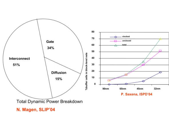
1.2 Total Dynamic Breakdown and % Buffer Cells in Block-Level Nets . . . 3

1.3 The Meaning of Fan Out from [25] . . . 4

1.4 Construct a Fanout Tree at The Source from [15] . . . 5

2.1 The Network from [12] . . . 8

2.2 The Delay Model from [15] . . . 10

3.1 The Elmore Delay from [25] . . . 12

3.2 The Original Example from [12] . . . 13

3.3 Two-Level Algorithm Step 1 . . . 18

3.4 Two-Level Algorithm Step 2 . . . 19

3.5 Two-Level Algorithm Step 3 . . . 20

3.6 The Building Process For Combinational Merging Tree . . . 21

3.7 Combinational Merging Algorithm Step 1 . . . 22

3.8 Combinational Merging Algorithm Step 2 . . . 23

3.9 Combinational Merging Algorithm Step 3 . . . 24

3.10 Combinational Merging Algorithm Step 4 . . . 25

3.11 Combinational Merging Algorithm Step 5 . . . 26

3.12 Combinational Merging Algorithm Step 6 . . . 27

List of Tables

4.1 Benchmark Information . . . 35

4.2 Simulation Results of the LT-Trees and Combinational Merging . . . 36

4.3 Simulation Results of the LT-Trees . . . 37

List of Algorithms

1 Buffer Insertion Algorithm . . . 16

2 Two-Level Algorithm . . . 28

3 Combinational Merging Algorithm . . . 31

4 LT-Trees Algorithm . . . 32

Chapter 1

Introduction

The buffer insertion and sizing are essential design methodologies for reducing interconnect delay [1]-[10]. In his past research [1], the VG algorithm has taken some important steps in this direction. The idea is to proceed bottom-up from the sink nodes along the tree toward the source node. During the bottom-up process, the set of candidate solutions at each node evolves through four operations (grow, add buffer, merge, prune solutions). The algorthm picks the best one from the solution set of the source and then top-down traverses the tree to get the corresponding buffer placement.

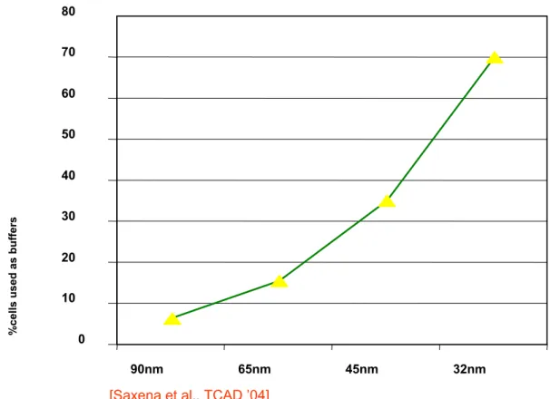
In Figure 1.1, almost 70% of the cell count on a chip will be the buffer at 32 nm process technology. Delay has a square dependence on the length of an RC unbuffered wire and buffers needed to linearize delay. For the interconnect optimization issue, the buffer insertion technique plays a very important role in DSM IC design: timing optimization, signal integrity and fixing of the various electrical violations (e.g. load, slew)[11]. In Figure 1.2, as we concern the inter-connect power, the power consumption in signal nets and the number of buffer are increasing drastically. The IC designers have actions needed to be taken: using optimal buffer to minimize the total power.

0 10 20 30 40 50 60 70 80 90nm 65nm 45nm 32nm % c

ells used as buffers

[Saxena et al., TCAD ’04]

0 10 20 30 40 50 60 70 80 90nm 65nm 45nm 32nm % buf fer c el ls in bl oc k-l ev el n ets clocked uncloced total P. Saxena, ISPD’04 Interconnect 51% Gate 34% Diffusion 15%

Total Dynamic Power Breakdown

N. Magen, SLIP’04

1.1

Motivation

source

sink

sink

sink

Fan-out N

Fig. 1.3: The Meaning of Fan Out from [25]

In order to make sure all that inputs of the logic gate still maintain the precise logic, the fanout optimization is the driving force behind VLSI design. The fanout is the number of load gates N that are connected to the output of the driving gate (see Figure1.3). On the other hand, the fanout is an unit of the ability of a logic gate output to drive a number of inputs of other logic gates of the same type. In most designs, logic gates are connected together to form more complex circuits, and it is common for one logic gate output to be connected to several logic gate inputs. Increasing the fanout of a gate can affect its logic output levels. Many library components define a maximum fanout to guarantee that the static and dynamic performance of the element meet the specification. In this thesis, considering interconnect delay, we will adopt the buffer insertion technique to synthesize the fanot tree which connects the source to the sink (see Figure 1.4) such that the require times at all the sinks are satisfied and the required time at the input pin of the source is maximized.

1.2

Our Contributions

In this thesis, we try to add interconnect delay in [12]. The interconnect delay could not be neglected because it will have huge impact on the design such as the number of buffer inserted, and the total delay. Considering the gate delay only will not get the correct result of the real world. Another contribution is the combination of the combinational merging algorithm and the LT-Trees algorithm because there is a trade-off between better solution and less time. The last contribution is to implement the retrace function that can be very easy to trace back the fanout tree structure.

1.3

Organization of the Thesis

The introduction, motivation, and contribution are in Chapter 1. Chapter 2 will have the previous works, and the problem formulation. The detail algorithm such as two-level algorithm, combinational merging algorithm, LT-Trees algorithm, and retrace algorithm will be explained clearly in Chapter 3. Finally, the experimental results and conclusion are given in Chapter 4 and Chapter 5, respectively.

Chapter 2

Preliminaries

2.1

Problem Formulation

Fig. 2.1: The Network from [12]

In [12], given a source s0 and n sinks s1, s2, .., sn, each sink has a required time r1, r2, .., rn

and an input pin capacitance c1, c2, .., cn, as shown in Figure 2.1. The buffer and gate at the

source are also provided in Figure 2.1. The delay of the buffer is dbuf = αbuf+ βbufCoutand the

are known constants. The Cout in buffer delay calculations is the sum total of the input pin

capacitances for all fanouts of the buffer. Another Cout involved in the gate delay is the sum

total of the input pin capacitances for all fanouts of the source. The problem is to evolve an algorithm to construct the fanout tree which connects the source to the sink (using the buffers as intermediate nodes) such that the required times at all the sinks are met, and the required time at the input pin of the source is maximized. The definition of the problem could be described more specifically as follows:

• Given a library of buffers with the same size: the input load Cbuf f er, the load dependent

delay βbuf f er and the intrinsic delay buffer αbuf f er.

• Given the source signal s, its drive capability βsourceand its intrinsic delay αsource

• Given n sinks with separate required times riand load Ci

• To find a tree of buffers that distributes the signal s to all the sinks and maximizes the

required time at the input end of source

2.2

Previous Works

• Effort-based delay equation:

™

τ : Semiconductor process parameter

™

p : Parasitic delay (due to diffusion cap.)

™

g : Logical effort (gate topology)

™

h : Electrical effort (gate size – L/C

)

L C_in

(

)

delay

=

τ

p gh

+

Fig. 2.2: The Delay Model from [15]

For the fanout optimization issue only, a paper provides such an approach: two-level, com-binational merging, LT-Trees algorithm under the discrete buffer size [13]. Considering the continuous buffer sizes issue [14] [15], they find that the fanout optimization result will be bet-ter than discrete buffer library. In [26], taking the gate sizing and fanout optimization at the same time, he claims that the optimization problem will be formulated as a non-convex optimization problem. Fanout optimization [22] is the problem of constructing a buffer tree topology be-tween a source and all sinks and the timing restrictions at all sinks are satisfied [13] [16] [19]. Several objective functions have been considered for the fanout optimization problem, such as minimizing area [16] [17] [18] [19], reducing power consumption [17] [19], and turning down load on the source [20].

In [15], they proposed an optimum solution for the single-sink buffering problem and de-veloped an effective heuristic for the multiple-sink fanout optimization problem. Specifically

speaking, they divide the input capacitance bound into a set of bounds for different source-sink pairs, solve the problem for each source-sink individually, merge all the source-sink pair solu-tions into a single fanout tree solution, discretize and map the logical buffers to physical buffers in the library. Figure 2.2 shows the delay model of their solution.

In [23], in their recent survey on repeater insertion, they have taken some important steps in this direction. A repeater insertion flow at different stages of back-end IC flow at circuit-level is presented. The main concern in this paper is what accuracy is required for the timing model at different stages of the flow and what stages establish the quality of the results. The flow was tested with very high-fanout nets. It is capable of simultaneously solving the problem of fanout optimization and repeater insertion during the back-end IC flow.

In [24], an algorithm was presented for delay optimization under the constraint of combina-tional logic, and they expand the state-of-the art sizing algorithm based on lagrangian relaxation. Moreover, tightly combining fanout tree build process, buffer insertion/sizing and gate sizing, they thereby accomplish more optimization than if they were performed independently.

Chapter 3

A Single Source Fanout Optimization

3.1

Interconnect Delay Model

A simple approximation to the delay in a RC network is elmore delay calculations used in logic synthesis very often. For the sake of the easy calculation and precise, the elmore delay model will be used to estimate the interconnect delay in this fanout optimization problem (see Figure 3.1).

Elmore Delay

2

2

2

1

1

(

)

)

(

A

C

R

C

C

R

C

Delay

−

=

+

+

A

R

B

R

C

C

C

3.2

The Original Example Without Interconnect Delay

Fig. 3.2: The Original Example from [12]

The fanout tree given in Figure 3.2(a) is adopted from [12]. The Cout=C1+C2+C3+C4+C5

that is the summation of all the capacitance at sink and the rout= minimum(r1,r2,r3,r4,r5), where

Ci is the input pin capacitance of node i and ri is the required time at the input of node i. The

required time at the input of the source is given by rsource = rout - dsource= rout - (αsource +

another topology solution in Figure 3.2(c) will look as follows: sink1 = source; buf1 = source; sink2 = buf1; buf2 = buf1; sink3 = buf2; buf3 = buf2; sink4 = buf3; sink5 = buf3;

The simple rule in output file is every net i with source node i and sink node j is represented as: node j= node i.

3.3

The Original Example With Interconnect Delay

We assume the net connecting any two nodes (source,sinks,buffers) will have the per-unit-resistance R and per-unit-capacitance C. In Figure 3(a), the required time at the input of the source rsource= rout- dsource= rout-(αsource+ βsourceCout ) has to be changed as follows rsource

= rout- dsource-R*C= rout-(αsource+ βsourceCout)-R*C.

In Figure 3(b), rbuf in=rbuf out-dbuf= rbuf out- (αbuf+βbufCbuf out) is necessary to be changed

as follows rbuf in =rbuf out-dbuf= rbuf out - (αbuf + βbufCbuf out) - R*C. The required time at the

3.4

The Algorithms Used In Fanout Optimization

Inputs: n sinks with required time ri, capacity Ci respectively, one source signal and a

one size buffer library αsource, βsource, αbuf f er, βbuf f er, Cbuf f er

per-unit-resistance,per-unit-capacitance

Output: maximum require time at source input and the buffer tree structure. begin

// The sorting algorithm used is quicksort, which is // not listed here. Sort the n sinks by increasing // required. If required time are the same, sorting // by decreasing capacity.

required = combine();

Ideal required time R0 = r1− αsource− βsource∗ (Cbuf f er+ C) − R ∗ (Cbuf f er+ C) − βbuf f erC1

if (R0 − required) < 10 then

output structure tree from the combinational merging; return required; exit(0); else required= LT( ); exit(0); end if end

H.Touati [13] proposed some methods to solve the one source fanout optimization problem in his dissertation. The dissertation shows in full detail how a single source fanout optimization is figured out by two-level, combinational merging, and LT-Trees (Algorithm 2 to 4).

1. Two-Level Trees:

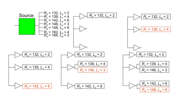
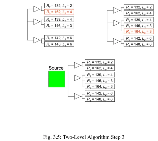
The characteristic of two-level trees is the usage of only one type of buffer. And even with this restricted tree structure, this optimization problem is NP-complete. The definition of two-level tree is that any leaf of this tree is separated from the root by only one node in this tree. A sink is set to an intermediate buffer only if this assignment reduces the required time at source at least. On the other hand , the algorithm chooses the allocation which maximizes the required time at the source node. The number of the intermediate node(buffer) could be defined as follows:qβbuf f er∗ sumC1/βsource∗ Cbuf f er. The sumC1is the sum of all sink’s capacity. The

time complexity of the algorithm (Algorithm 2) is O(n1.5). This is a greedy algorithm which does not guarantee optimality, but is a baseline algorithm for other more sophisticated methods. In algorithm 1, the required time at all sink is sorted by quick sort and the capacity is the second key in quick sort when two of the required time are the same value. Figure 3.3 to Figure 3.5 show that that the construct process of the two-level tree.

2. Combinational Merging:

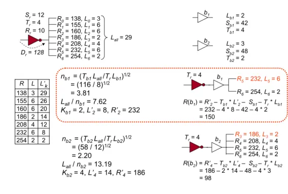
The algorithm incrementally inserts buffer cells and connects the k sink nodes with the largest required times. For combinational merging (Algorithm 3), the method is presented as follows: To sort the n sinks by ascending required times, to link the n-k+1 sinks with the largest require times to a buffer, to merge the new buffer node with the left k-1 sinks to generate a new k nodes sorted array. The procedure must be done recursively, until the k is equal to 1.

0 0 6 L’i ∞ ∞ 2 ∞ ∞ 1 72 132 0 R’i Rmini buf R₀= 132, L₀= 2 Rr= 24 R1= 139, L1= 4 R’₀ R’₁ R’₂ D’r= 48 R₀= 132, L₀= 2 R_r= 32 R1= 139, L1= 4 R’0 R’1 R’2 D’_r= 48 MIN { R’₀, R’₁, R’₂ } = 72 MIN { R’0, R’1, R’2 } = 80

This is a better allocation

0 4 2 L’i ∞ ∞ 2 83 139 1 80 132 0 R’i Rmini buf

R’

=

Rmin0 –

β

* load – Sb

R0= 132, L0= 2 R1= 139, L1= 4 R₂= 142, L₂= 6 R4= 148, L4= 6 R3= 146, L3= 3 R6= 164, L6= 3 R₅= 162, L₅= 4 Source R0= 132, L0= 2 R₀= 132, L₀= 2 R1= 139, L1= 4 R0= 132, L0= 2 R1= 139, L1= 4 R₂= 142, L₂= 6 R0= 132, L0= 2 R1= 139, L1= 4 R₂= 142, L₂= 6 R3= 146, L3= 3 R0= 132, L0= 2 R1= 139, L1= 4 R₂= 142, L₂= 6 R3= 146, L3= 3 R4= 148, L4= 6

R₀= 132, L₀= 2 R₁= 139, L₁= 4 R₂= 142, L₂= 6 R₃= 146, L₃= 3 R4= 148, L4= 6 R₅= 162, L₅= 4 R₀= 132, L₀= 2 R1= 139, L1= 4 R2= 142, L2= 6 R₃= 146, L₃= 3 R₄= 148, L₄= 6 R₅= 162, L₅= 4 R6= 164, L6= 3 R0= 132, L0= 2 R₁= 139, L₁= 4 R₂= 142, L₂= 6 R3= 146, L3= 3 R4= 148, L4= 6 R5= 162, L5= 4 R₆= 164, L₆= 3 Source

1. Sort the sinks in the increasing order of their required times (in case of a tie, the decreasing order of the gate load)

2. For each buffer cell b_j, compute the optimal number of sinks k_bj(from the tail of the sink list) to be connected to b_j.

— Lall: total gate loads in the sink list

— nbj= (TjLall/TrLj)1/2 : optimal number of buffers in two-level tree using cell

bj

— L_all/ n_bj: Optimal load per single buffer b_j

— L’_k：total gate loads of the last k nodes in the sink list ¾ kbjis the smallest k which satisfies L’k≥ Lall/ nbj

3. For each cell type b_j, let R(b_j) be the required time at the source r where only a single cell of b_jis connected to r and cell b_jis connected to the last k (= k_bj) nodes in the sink list.

— R(b_j) = R’_k– T_bjL_k– S_bj– T_rL_bj

— R’_k：required time of the k-th node from the bottom of the sink list

¾ Choose the cell type bjwhich gives the largest R(bj)

(this will have the largest speed up effect)

4. Update sink list :

¾ Insert the cell b_jto the fan-out tree

¾ Delete the kbjnodes from the sink list (since they are buffered by bj)

¾ Add b_jto the sink list

— Required time at the inserted b_jcell : R(b_j) = R’_k– T_bjL_k– S_bj

¾ If kbjis less than the total number of nodes in the sink list, go to 1. 5. Retrieve the best allocation during the whole process (allocation with • Fan-out optimization： Construct a fan-out tree which maximize the required

time R_rat the net source r on following conditions

– Net source r :

• Output transition coefficient : T_r

(Switching delay Sris not really needed in the optimization) – Buffer cell b_j:

• Gate load : L_bj • Switching delay : Sbj

• Output transition coefficient : T_bj

– Sink i (i = 1, 2, … n)

• Gate load : Li

2 2 254 8 6 232 12 4 208 14 2 186 20 6 160 26 6 155 29 3 138 L’_k L R nb1 = (Tb1 Lall/TrLb1) 1/2 = (116 / 8)1/2 = 3.81 Lall/ nb1= 7.62 K_b1= 2, L’₂= 8, R’₂= 232 b1 _L b1= 2 S_b1= 42 T_b1= 4 b_{2 L} b2= 3 Sb2= 48 Tb2= 2 R(b₁) = R’₂– T_b1* L’₂– S_b1 – T_r* L_b1 = 232 – 4 * 8 – 42 – 4 * 2 = 150 R(b₂) = R’₄– T_b2* L’₄– S_b2 – T_r* L_b2 = 186 – 2 * 14 – 48 – 4 * 3 = 98 T_r= 4 Lall= 29 S_r= 12 R0= 138, L0= 3 R₁= 155, L₁= 6 R2= 160, L2= 6 R₄= 208, L₄= 4 R3= 186, L3= 2 R6= 254, L6= 2 R5= 232, L5= 6 R_r= 10 D_r= 128 nb2 = (Tb2 Lall/TrLb2)1/2 = (58 / 12)1/2 = 2.20 L_all/ n_b2= 13.19 Kb2= 4, L’4= 14, R’4= 186 b1 Tr= 4 R₆= 254, L₆= 2 R5= 232, L5= 6 b2 T_r= 4 R₆= 254, L₆= 2 R₅= 232, L₅= 6 R4= 208, L4= 4 R₃= 186, L₃= 2

14 2 158 4 4 208 6 2 186 12 6 160 20 6 155 23 3 138 L’_k L R nb1 = (Tb1 Lall/TrLb1) 1/2 = (92 / 8)1/2 = 3.39 L_all/ n_b1= 6.78 K_b1= 3, L’₃= 12, R’₃= 160 b_{1 L} b1= 2 S_b1= 42 Tb1= 4 b2 _L b2= 3 Sb2= 48 Tb2= 2 R(b1) = R’3– Tb1* L’3– Sb1 – Tr* Lb1 = 160 – 4 * 12 – 42 – 4 * 2 = 62 R(b₂) = R’₃– T_b2* L’₃– S_b2 – T_r* L_b2 = 160 – 2 * 12 – 48 – 4 * 3 = 76 T_r= 4 Lall= 23 S_r= 12 R0= 138, L0= 3 R1= 155, L1= 6 R2= 160, L2= 6 R₄= 208, L₄= 4 R3= 186, L3= 2 R_r= 34 D_r= 104 nb2 = (Tb2 Lall/TrLb2)1/2 = (46 / 12)1/2 = 1.96 L_all/ n_b2= 11.75 Kb2= 3, L’3= 12, R’3= 160 R_b0= 158, L_b0= 2 b1 R6= 254, L6= 2 R₅= 232, L₅= 6 b2 T_r= 4 R4= 208, L6= 4 R₃= 186, L₅= 2 R2= 172, L4= 6 b₁ Tr= 4 R₄= 208, L₆= 4 R3= 186, L5= 2 R₂= 172, L₄= 6

14 3 100 2 2 158 8 6 155 11 3 138 L’_k L R nb1 = (Tb1 Lall/TrLb1) 1/2 = (56 / 8)1/2 = 2.65 Lall/ nb1= 5.29 K_b1= 2, L’₂= 8, R’₂= 155 b_{1 L} b1= 2 S_b1= 42 T_b1= 4 b2 _L b2= 3 Sb2= 48 Tb2= 2 R(b1) = R’2– Tb1* L’2– Sb1 – Tr* Lb1 = 155 – 4 * 8 – 42 – 4 * 2 = 73 R(b₂) = R’₃– T_b2* L’₃– S_b2 – T_r* L_b2 = 138 – 2 * 11 – 48 – 4 * 3 = 56 T_r= 4 Lall= 14 S_r= 12 R₀= 138, L₀= 3 R1= 155, L1= 6 R_r= 32 D_r= 68 nb2 = (Tb2 Lall/TrLb2)1/2 = (28 / 12)1/2 = 1.53 L_all/ n_b2= 9.17 Kb2= 3, L’3= 11, R’3= 138 Rb0= 158, Lb0= 2 Rb1= 88, Lb1= 3 b1 R6= 254, L6= 2 R₅= 232, L₅= 6 b₂ R₄= 208, L₄= 4 R3= 186, L3= 2 R₂= 160, L₂= 6 b1 T_r= 4 Rb0= 158, Lb0= 2 R1= 155, L4= 6 b₂ Tr= 4 RR_b01= 158, L= 155, L_b05= 6= 2 R₀= 132, L₄= 3

8 2 81 6 3 88 3 3 138 L’_k L R nb1 = (Tb1 Lall/TrLb1) 1/2 = (32 / 8)1/2 = 2.00 L_all/ n_b1= 4.00 K_b1= 2, L’₂= 6, R’₂= 88 R(b1) = R’3– Tb1* L’3– Sb1 – Tr* Lb1 = 88 – 4 * 6 – 42 – 4 * 2 = 14 R(b₂) = R’₃– T_b2* L’₃– S_b2 – T_r* L_b2 = 81 – 2 * 8 – 48 – 4 * 3 = 5 T_r= 4 L_all= 8 S_r= 12 R0= 138, L0= 3 R_r= 37 D_r= 44 nb2 = (Tb2 Lall/TrLb2)1/2 = (16 / 12)1/2 = 1.15 L_all/ n_b2= 6.93 Kb2= 3, L’3= 8, R’3= 81 Rb1= 88, Lb1= 3 R_b2= 81, L_b2= 2 _{Rb0= 158, Lb0= 2} b1 R₆= 254, L₆= 2 R5= 232, L5= 6 b₂ R₄= 208, L₄= 4 R3= 186, L3= 2 R₂= 160, L₂= 6 b1 R₁= 155, L₁= 6 b₁ Tr= 4 R₀= 132, L₀= 3 R_b1= 100, L_b1= 3 b2 T_r= 4 R0= 132, L0= 3 RR_b1b2= 100, L= 81, Lb2_b1= 2= 3

4 2 22 2 2 81 L’_k L R nb1 = (Tb1 Lall/TrLb1) 1/2 = (16 / 8)1/2 = 1.41 L_all/ n_b1= 2.83 Kb1= 2, L’2= 4, R’2= 22 R(b₁) = R’₂– T_b1* L’₂– S_b1 – T_r* L_b1 = 22 – 4 * 4 – 42 – 4 * 2 = – 44 R(b2) = R’3– Tb2* L’3– Sb2 – Tr* Lb2 = 22 – 2 * 4 – 48 – 4 * 3 = – 46 Tr= 4 Lall= 4 Sr= 12 Rr= – 6 Dr= 28 n_b2 = (T_b2 L_all/T_rL_b2)1/2 = (8 / 12)1/2 = 0.82 Lall/ nb2= 4.90 K_b2= 2, L’₂= 4, R’₂= 22 Rb3= 22, Lb3= 2 _R 0= 138, L0= 3 Rb1= 100, Lb1= 3 b₂ R₄= 208, L₄= 4 R3= 186, L3= 2 R₂= 160, L₂= 6 R_b2= 81, L_b2= 2 _{Rb0= 158, Lb0= 2} b1 R₆= 254, L₆= 2 R5= 232, L5= 6 b1 R₁= 155, L₁= 6 b₁ b1 Tr= 4 R_b2= 81, L_b2= 2 R_b3= 34, L_b3= 2 b1 T_r= 4 Rb2= 81, Lb2= 2 Rb3= 34, Lb3= 2

T_r= 4 S_r= 12 R_r= – 44 D_r= 20 R₀= 138, L₀= 3 b₂ R4= 208, L4= 4 R3= 186, L3= 2 R₂= 160, L₂= 6 b_{1 R}R₆5_{= 254, L}= 232, L₆5_{= 2}= 6 b1 R₁= 155, L₁= 6 b₁ b₁ R=158 R=88 R=22 R=81 Tr= 4 Sr= 12 Rr= 37 Dr= 44 R0= 138, L0= 3 b2 R4= 208, L4= 4 R₃= 186, L₃= 2 R2= 160, L2= 6 b1 R₆= 254, L₆= 2 R5= 232, L5= 6 b1 _{R1= 155, L1= 6} R=158 R=88 R=81 T_r= 4 Sr= 12 Rr= 6 Dr= 28 R₀= 138, L₀= 3 b₂ R₄= 208, L₄= 4 R3= 186, L3= 2 R₂= 160, L₂= 6 b1 R6= 254, L6= 2 R5= 232, L5= 6 b1 R₁= 155, L₁= 6 b1 R=158 R=88 R=22 R=81 Tr= 4 Sr= 12 Rr= 32 Dr= 68 R₀= 138, L₀= 3 b2 R4= 208, L4= 4 R₃= 186, L₃= 2 R2= 160, L2= 6 b_{1 R}R₆5_{= 254, L}= 232, L₆5_{= 2}= 6 R1= 155, L1= 6 R=158 R=88 Tr= 4 Sr= 12 Rr= 34 Dr= 104 R₀= 138, L₀= 3 R4= 208, L4= 4 R3= 186, L3= 2 R2= 160, L2= 6 b_{1 R}R₆5_{= 254, L}= 232, L₆5_{= 2}= 6 R₁= 155, L₁= 6 R=158 T_r= 4 S_r= 12 R_r= 10 D_r= 128 R0= 138, L0= 3 R₄= 208, L₄= 4 R3= 186, L3= 2 R2= 160, L2= 6 R₆= 254, L₆= 2 R5= 232, L5= 6 R1= 155, L1= 6

Algorithm 2 Two-Level Algorithm

Inputs: from sink k+1 to sink n , sorted by ascending required time, the capacity of these (n-k+1) sinks(Ck+1, Ck+2...Cn), the sum of the capacity of these (n-k) sinks,sumCk

αsource, βsource, αbuf f er, βbuf f er, Cbuf f erper-unit-resistance,per-unit-capacitance

Output: the required time of the (n-k) sinks using two-level fanout tree begin

//if k is zero, the root is the source, otherwise, the root is buffer beta = ( k==0)? βsource:βbuf f er

// calculating the number of buffers needed nBuffer =qβbuf f er∗ sumC1/βsource∗ Cbuf f er

//the number of buffers will less than the number of sinks nBuffer =((nBuf f er) < (n − k))?nBuffer:(n-k)

//rBuffer stands for Cout and lBuffer represents //Cbuf

for i=1 to nBuffer do

rBuffer[i] =0.0; lBuffer[i] =0.0;

end for

temp = -1000000;

//assign sink to buffer begin with the one with // biggest required time, easy to calculate the // buffer require time

for i=n to k+1 do for j=1 to nBuffer do

// the new added one has the minimum // require time

required = ri− βbuf f er∗ (lBuf f er[j] + Ci)-PerUnitInterconnectDelay;

if (temp) < (required) then

temp =required; num =j ; end if end for rBuffer[num] = temp; lBuffer[num] = lBuffer[num]+Ci; end for for i =1 to nBuffer do

result = (result < rBuf f er[i]) ?result : rBuffer[i]; result = result- ( β ∗ Cbuf f er∗ nBuf f er) − (αbuf f er);

end for

return result; end

3. LT-Trees: The two-level trees can only build restricted type of net structure, which is not efficient and sufficient if the required times at sinks are very different from each other. The combinational merging is only using a heuristic approach to choose the parameter k. The LT-trees algorithm is a compromised algorithm between combinational merging and two-level fanout trees. The definition of the LT-trees [13]:

a. A leaf is an LT-Tree

b. A two-level tree is an LT-Tree

c. Let T be a tree rooted at r such that one child of r is an LT-Tree and all the other children of r are leaves. Then T is an LT-Tree.

If a node has more than one child being intermediate node, we only consider it as a two-level trees. Compared to the trees structure constructed by two-level trees and combinational merg-ing, the trees structure defined above is much more complex, making it possible to handle the situation as sinks have very big capacities or/and the required times of sinks are very different from each other. On the other hand, the LT-trees are only a small subset of the set of all fanout trees, making it practical in general use. This algorithm is also not optimal based on the sorting of sinks by increasing required times. The complexity of it is O(n2.5). The Figure 3.13 shows the construct of LT-Trees.

The LT-trees algorithm uses the dynamic programming to generate the optimal LT-Trees for a given fanout problem. The idea is: For k from n to 1, each k is also a fanout problem.

1. First compute the two-level trees on k

2. As induction on k from n to 1, for any m > k, the optimal LT-trees T(m) is already known. Connect sink k, k+1,....,m-1 and optimal LT-tree T(m) to root, obtain the relative required time. 3. The final optimal LT-tree T(k) is the one from step 1 and 2 with the maximum required

The fanout optimization is a NP-Complete problem if non-constant capacity values are al-lowed at sinks. So, there is always a trade-off between better solution and less time. combina-tional merging algorithm is a heuristic algorithm with much less time consumed than LT-Trees algorithm. In this thesis, the two algorithms are combined: We already know the minimum re-quired time at sinks and we can get the ideal maximum rere-quired time by: r1− αsource− βsource∗

(Cbuf f er+ C) − R ∗ (Cbuf f er + C) − βbuf f erC1

For each benchmark, we first use the combinational merging algorithm, and if the obtained required time is within a small range of the ideal required time, computing stops here. Other-wise, the LT-Trees algorithm will be called for a better solution. Since combinational merging is very fast, its overhead on those using LT-Trees finally is acceptable.

R0= 132, L0= 2 R₁= 139, L₁= 4 R2= 142, L2= 6 R₄= 148, L₄= 6 R3= 146, L3= 3 R6= 164, L6= 3 R₅= 162, L₅= 4 Source R_{0 R} 5 R1 R3 R2 R4 R₆ Source

Algorithm 3 Combinational Merging Algorithm

Inputs: n sinks sorted by ascending required time , one source signal and a one size buffer libraryαsource, βsource, αbuf f er, βbuf f er, Cbuf f er per-unit-resistance,per-unit-capacitance

Output:maximum require time at source input and the buffer tree structure int n= nSink; double kopt;

int k; int step=0; double rt;

while n > 0 do for i=0 to n do

sumC[i]=0.0;

for int j=i to n do

sumC[i]+=cSink[j];

end for end for

kopt = sqrt(bBuffer*sumC[0]/(bSource*cBuffer));

for i= 0 to n do

if sumC[i] > (sumC[0]/kopt) then

k=i; end if end for rt= rSink[k]-bBuffer*sumC[k]-aBuffer-PerUnitInterconnectDelay; for i=k to n do pSink[sSink[i]]=(k==0)?-1:step; end for if k == 0 then break; end if quicksort(rSink,cSink,sSink,0,k); int i=0; for i=0 to k do if rSink[i] > rt then break; end if end for if i==k then rSink[k]=rt; cSink[k]=cBuffer; sSink[k]=nSink+step;

Algorithm 4 LT-Trees Algorithm

Inputs: n sinks sorted by ascending required time one source signal and a one size buffer library. αsource, βsource, αbuf f er, βbuf f er, Cbuf f er per-unit-resistance,per-unit-capacitance

Output: maximum require time at source input and the buffer tree structure. begin for i=1 to n do for j= i to n do sumCi = sumCi+ Cj; end for end for sumCn+1= Cbuf f er; required[n+1] =Cn+1000 for i=n to 1 do required[i] = two-level(); tLevel[i] = true; for j=i+1 to n+1 do

// calculating the required time when the sink k to // to sink(j-1) connected to root directly.

// rk is the smallest required time temp =min(rk, required[j] − αbuf f er)

temp -= ((i == 1)?βsource : βbuf f er) * (Cbuf f er + sumCk − sumC1

)-PerUnitInterconnectDelay;

if (temp > required[i]) then

required[i] = temp; tLevel[i] = false; next[i] = 1 end if end for end for

required[1] = (αsource)-(required[1]);

call the retrace function;

return required[1] and the L-T structure end

Algorithm 5 Retrace Algorithm

Inputs: boolean tLevel[k], k=1,2...n, for each k, if two-level is used int next[k], k=1,2,....n, the first sink that does not connected to root directly

Output: the total number of buffer nBuffer, the parent node for each sink pSink[k], the parent node for each buffer pBuffer[i], i=1,2...nBuffer

begin

int step = -1; int i = 0;

while (i) < (n + 1) do if tLevel[i]==true then

run two-level algorithm to get nBuffer and the num for each sink

for i=n to k+1 do for j=1 to nBuffer do pBuffer[step+1+j] = step; end for pSink[i] = step+1+num; end for

nBuffer = nBuffer + step+1; break;

else

for j=i to(next[i] - 1) do

pSink[j]=step; pBuffer[step+1]=step; end for end if step++; i=next[i]; end while end

Chapter 4

Experimental Results

The whole algorithms are implemented in C++ and the platform used for this master thesis is Pentium 4 2.66 GHz, 1280MB dram. The parameter of the resistance and the per-unit-capacitance are gotten from [10]. We will adopt interconnects per unit length for every connects between nodes.

There are three output files :

1. The number and the name of the buffer used.

2. The net information among these nodes:source, sink, buffer. 3. The runtime for each benchmark and relative information.

The information for each benchmark are shown in Table 4.1. In Table 4.2 to Table 4.4, the Minimum is the minimum required time at sinks, the Original stands for the required time at source without buffer insertion, the Ideal represents the potential best required time, the Result on behalf of the final result at source after buffer insertion, and the NBuffer is the usage of buffer number for every benchmark. The simulation results are shown in Table 4.2 to Table 4.4. While a great number of papers have been written on the fanout optimization, many of them entirely do not consider the interconnect delay issue.

The * symbol in Table 4.2 to Table 4.4 is the whole algorithm running with consideration of the interconnect delay. Once the delay value in Table 4.2 to Table 4.4 has been changed, the number of the buffer is also different from that without interconnect delay. The result** means that we check the timing for every sink to source and choose the smallest one.

Besides the field of Method, NBuffer and Runtime in Table 4.2 to Table 4.4, the unit of every field in the Table 4.2 to Table 4.4 is picosecond. For each benchmark, we first use the

Table 4.1: Benchmark Information Bench1 Bench2 Bench3 Bench4 Bench5

αsource 1 1 1 1 1 βsource 0.5 0.5 0.5 0.5 0.5 αbuf 1 1 1 1 1 βbuf 0.5 0.5 0.5 0.5 0.5 Cbuf 1 1 1 1 1 Total Sinks 1000 2000 3000 4000 5000 Bench6 Bench7 Bench8 Bench9 Bench10

αsource 1 1 1 1 1 βsource 0.5 0.5 0.5 0.5 0.5 αbuf 1 1 1 1 1 βbuf 0.5 0.5 0.5 0.5 0.5 Cbuf 1 1 1 1 1 Total Sinks 6000 7000 8000 9000 10000

combinational merging algorithm, and if the obtained required time is within a small range of the ideal required time, computing stops here. Otherwise, the LT-Trees algorithm will be called for a better solution. Since combinational merging algorithm is efficient, its overhead on those using LT-Trees algorithm finally is acceptable. Adding the interconnect delay results in the usage of decreasing the number of buffer.

Table 4.2: Simulation Results of the LT-Trees and Combinational Merging Bench1 Bench2 Bench3 Bench4 Bench5

Minimum 70265 76067 70265 80005 80000 Original 68933 73404 66271 74071 72726 Ideal 70263 76063 70263 80002 79998 Result 70263 76056 70258 80002 79997 Result** 70262 75993 70139 80001 79995 Result* 70257 76036 70241 79997 79991 Delay 2.0221 10.9944 7.8357 2.0005 3 Delay* 8.0672 30.8928 24.0712 7.5015 8.5008 NBuffer 493 135 168 2497 3062 NBuffer* 476 136 168 1422 1488 Runtime 0.2810 0.5150 2.3590 8.3760 13.1720 Runtime* 0.2970 0.5160 2.4840 8.8280 15.2040 Method LT-TREES C.M. C.M. LT-TREES LT-TREES

Bench6 Bench7 Bench8 Bench9 Bench10 Minimum 80000 76067 70265 80000 80000 Original 71285 66749 59617 67179 65651 Ideal 79998 76064 70263 79998 79998 Result 79997 76054 70259 79997 79996 Result** 79996 75893 70145 79996 79995 Result* 79990 76035 70241 79990 79989 Delay 2.1653 12.2716 6.4508 2.7819 3.0004 Delay* 9.0013 31.8043 24.4905 9.5019 10.5032 NBuffer 3363 267 288 3177 2598 NBuffer* 1415 267 288 1004 802 Runtime 20.3440 23.2660 28.2660 54.8600 71.7190 Runtime* 23.7810 24.4060 29.6400 64.1880 84.0940 Method LT-TREES C.M. C.M LT-TREES LT-TREES

Table 4.3: Simulation Results of the LT-Trees

Bench1 Bench2 Bench3 Bench4 Bench5 Minimum 70265 76067 70265 80005 80000 Original 68933 73404 66271 74071 72726 Ideal 70263 76063 70263 80002 79998 Result 70263 75994 70140 80002 79997 Result** 70262 75993 70139 80001 79996 Result* 70257 75970 70097 79997 79991 Delay 2.0221 72.7322 125.2144 2.0005 3 Delay* 8.0672 96.1278 168.1960 7.5015 8.5008 NBuffer 493 980 671 2497 3062 NBuffer* 476 868 622 1422 1488 Runtime 0.2660 1.0780 2.3590 7.7970 13.3900 Runtime* 0.2970 1.2510 3.7650 8.7660 15.1570 Method LT-TREES LT-TREES LT-TREES LT-TREES LT-TREES

Bench6 Bench7 Bench8 Bench9 Bench10 Minimum 80000 76067 70265 80000 80000 Original 71285 66749 59617 67179 65651 Ideal 79998 76063 70263 79998 79998 Result 79997 75894 70146 79997 79996 Result** 79996 75893 70145 79996 79995 Result* 79990 75860 70097 79990 79989 Delay 2.1653 172.3098 119.2462 2.7819 3.0004 Delay* 9.0013 206.2102 167.9518 9.5019 10.5032 NBuffer 3363 1039 2872 3177 2598 NBuffer* 1415 979 1662 1004 802 Runtime 21 27.6410 28.2660 57.2660 74.7810 Runtime* 23.7030 31.3600 43.5790 64.5310 83.7650

Table 4.4: Simulation Results of Combinational Merging Bench1 Bench2 Bench3 Bench4 Bench5

Minimum 70265 76067 70265 80005 80000 Original 68933 73404 66271 74071 72726 Ideal 70263 76063 70263 80002 79998 Result 70263 76056 70258 80002 79995 Result** 70262 75993 70139 80001 79996 Result* 70251 76036 70241 79993 79985 Delay 2.0221 10.9944 7.0167 2.000500 4.5008 Delay* 14.0221 30.8928 24.0712 11.0145 14.5000 NBuffer 100 135 168 215 237 NBuffer* 100 136 168 215 237 Runtime 0.2810 0.5160 2.438 8.3440 14.11 Runtime* 0.2800 0.5320 2.469 8.2810 14.4680 Method C.M. C.M. C.M. C.M. C.M. Bench6 Bench7 Bench8 Bench9 Bench10 Minimum 80000 76067 70265 80000 80000 Original 71285 66749 59617 67179 65651 Ideal 79998 76064 70263 79998 79998 Result 79996 76054 70259 79995 79996 Result** 79996 75893 70145 79996 79995 Result* 79981 76035 70241 79982 79980 Delay 3.1653 12.2716 6.4508 4.0002 4.1379 Delay* 18.1657 31.8043 24.4905 17.5104 19.5010 NBuffer 260 267 288 317 337 NBuffer* 260 267 288 317 337 Runtime 22.1412 24.1876 29.1253 60.9537 80.7813 Runtime* 22.6720 24.4060 29.8280 61.7660 82.9230 Method C.M. C.M. C.M C.M. C.M.

Chapter 5

Conclusion

The fanout optimization is a NP-Complete problem if non-constant capacity values are allowed at sinks. There is always a trade-off between better solution and less time. Combina-tional Merging Algorithm is a heuristic algorithm with much less time consuming than LT-Trees Algorithm. In this thesis, the two algorithms are combined: We already know the minimum re-quired time at sinks and we can get the ideal maximum rere-quired time by: Ideal rere-quired time:

r1 − αsource− βsource∗ (Cbuf f er+ C) − R ∗ (Cbuf f er + C) − βbuf f erC1

For each benchmark, we first use the combinational merging algorithm, if the obtained re-quired time is within a small range of the ideal rere-quired time, computing stops here. Otherwise, LT-Trees algorithm will be called for a better solution. Since combinational merging is very fast, its overhead on those using LT-Trees finally is acceptable.

The interconnect delay could not be neglected in deep sub-micron IC design. In this thesis, the interconnect delay is elmore delay model. The future works will include the extension of gate sizing, one more size buffer library, multiple sink, more precise model of source gate model and interconnect delay. At last, the improvement of the benchmark will have the X-Y information for every node including buffer, source, sink that can estimate the length of

Bibliography

[1] L. P. P. P. van Ginneken, “ Buffer placement in distributed RC-tree networks for minimal Elmore delay,” in In Proc. Intl. Symposium on Circuits and Systems, pp. 865-868,1990. [2] H. Bakoglu, “ Circuits, Interconnections, and Packaging for VLSI,” Addison-Wesley

Pub-lishing Company,1987.

[3] J. Lillis, C. K. Cheng and T.-T. Y. Lin, “ Optimal wire sizing and buffer insertion for low power and a generalized delay model,” in IEEE J. Solid-State Circuits, vol. 31(3), pp.

437-447,1996.

[4] Weiping Shi and Zhuo Li, “ A Fast Algorithm for Optimal Buffer Insertion,” in IEEE

Trans. Computer-Aidede Design, vol. 24, no. 6, pp. 879-891.,June 2005.

[5] Weiping Shi and Zhuo Li, “ An O(nlogn) Time Algorithm for Optimal Buffer Insertion,”

in 40th Design Automation Conference (DAC), pp. 580-585, 2003.

[6] Zhuo Li and Weiping Shi, “ An O(bn2) Time Algorithm for Optimal Buffer Insertion with b Buffer Types,” in Conference on Design, Automation and Test in Europe (DATE),

Munich, Germany, pp. 1324-1329, March 2005.

[7] Weiping Shi, Zhuo Li and Charles J. Alpert, “ Complexity Analysis and Speedup Tech-niques for Optimal Buffer Insertion with Minimum Cost,” in 9th Asia and South Pacific

Design Automation Conference (ASP-DAC), Yokohama, Japan, pp. 609-614, Jan 2004.

[8] Zhuo Li, C. N. Sze, Charles J. Alpert, Jiang Hu and Weiping Shi, “ Making Fast Buffer In-sertion even Faster via Approximation Techniques,” in 10th Asia and South Pacific Design

[9] Zhuo Li and Weiping Shi, “ An O(mn) Time Algorithm for Optimal Buffer Insertion of Nets with m Sinks,” in 11st Asia and South Pacific Design Automation Conference

(ASP-DAC), Yokohama, Japan, pp. 320-325., Jan 2006.

[10] “Fast Buffer Insertion Source Code,”

[11] Y. Peng and X. Liu, “ Low-power repeater insertion with both delay and slew rate con-straints ,” in DAC, pp. 303-307, 2006.

[12] “ http://www.ece.umd.edu/class/enee644.S2004/project/project.htm,”

[13] H. Touati, “ Performance-oriented technology mapping ,” in Ph.D. dissertation, Univ.

California, Berkeley, CA, 1990.

[14] D. Kung, “ A Fast Fanout Optimization Algorithm for Near- Continuous Buffer Libraries ,” Proc. of 35th DAC, pp. 352-355 , June 1998.

[15] P. Rezvani, A. Ajami, M. Pedram, H. Savoj, “ Leopard: A Logical Effort-based fanout Optimization for Area and Delay ,” Proc. of ICCAD, pp. 516-519 , November 1999. [16] P. Rezvani and M. Pedram, “ A fanout optimization algorithm based on the effort delay

model,” IEEE Trans. Comput.-Aided Design Integr. Circuits Syst., vol. 22, no. 12, pp.

1671-1678, Dec. 2003.

[17] D. Zhou and X. Liu,“ Minimization of chip size and power consumption of high-speed VLSI buffers,” in Proc. Int. Symp. Phys.pp. 186-191, Dec.1997.

prob-[21] K. Kodandapani, J. Grodstein, A. Domic, and H. Touati,“ A simple algorithm for fanout optimization using high-performance buffer libraries,” in Proc. Int. Conf. Comput.-Aided

Des. pp. 466-471, 1993.

[22] B. Amelifard, F. Fallah, and M. Pedram,“Low-power fanout optimization using multi threshold voltages and multi channel lengths,” IEEE Trans. on Computer Aided Design,,

Vol. 28, No. 4, pp.478-489, Apr. 2009.

[23] Nikolai Ryzhenko, Oleg Venger,“A Practical Repeater Insertion Flow,” GLSVLSI08

pp.261-266, May 2008.

[24] I-Min Liu, Adnan Aziz, “ Delay Constrained Optimization by Simultaneous Fanout Tree Construction, Buffer InsertiodSizing and Gate Sizing ,” Proceedings of the 37th annual

ACM/IEEE Design Automation Conference pp.209-214, June 2000.

[25] Jan M. Rabaey, Anantha Chandrakasan, and Borivoje Nikolic, “ Digital Integrated Circuits (2nd Edition),” pp. 25-26,Jan 2003.

[26] Wei Chen, Cheng-Ta Hsieh, Massoud Pedram, “ Simultaneous Gate Sizing and Fanout Optimization,” Proceedings of the 2000 IEEE/ACM international conference on Computer