使用金屬平衡演算法來降低時鐘樹架構受製程變數的影響

國

立

交

通

大

學

電子工程學系 電子研究所碩士班

碩

士

論

文

使用金屬平衡演算法來降低時鐘樹架構受製程變數的影響

On Tolerating Process Variation with Metal Balance in Clock Tree

Construction

研 究 生：陳智偉

指導教授：陳宏明 博士

使用金屬平衡演算法來降低時鐘樹架構受製程變數的影響

On Tolerating Process Variation with Metal Balance in Clock Tree

Construction

研 究 生：陳智偉 Student：Zhi-Wei Chen

指導教授：陳宏明 博士 Advisor：Dr. Hung-Ming Chen

國 立 交 通 大 學

電子工程學系 電子研究所碩士班

碩 士 論 文

A Thesis

Submitted to Department of Electronics Engineering & Institute of Electronics College of Electrical and Computer Engineering

National Chiao Tung University in partial Fulfillment of the Requirements

for the Degree of Master

in

Electronics Engineering October 2008

Hsinchu, Taiwan, Republic of China

使用金屬平衡演算法來降低時鐘樹架構受製程

變數的影響

學生 : 陳智偉 指導教授 : 陳宏明 教授

國立交通大學 電子工程學系 電子研究所碩士班

摘 要

隨著製程技術的進步，我們越來越難達到零偏斜或接近零偏斜的時鐘

分配，即使經過一些常見的演算法來合成零偏斜的時鐘。在本篇論文

中，我們提出了一個方法，透過平衡各金屬層的繞線長，來增強時鐘

架構對製程變數的抗性。由實驗結果可以得知，我們的方法使用在無

插入緩衝器和插入緩衝器兩種時鐘樹合成，能比 DME 演算法更有效的

降低因製程變數所產生的偏斜。

On Tolerating Process Variation with Metal Balance in Clock Tree

Construction

Student: Zhi-Wei Chen

Advisor: Prof. Hung-Ming Chen

Department of Electronics Engineering

Institute of Electronics

National Chiao Tung University

ABSTRACT

With advanced manufacturing technology, it is getting difficult to have zero or almost zero-skew clock distribution, even the clock is synthesized to be zero-skew from conventional algorithms. In this work, we proposed a practical problem in clock construction with process variation awareness, which is to achieve the balance of the wirelength in preferred direction metal routing. Experimental results show that our approach (unbuffered and buffered clock tree syntheses) performs better than conventional DME algorithms in reducing the skew of the clock.

致 謝

能完成這篇論文，當然最感謝的就是指導教授陳宏明教授，教授

兩年來的關懷和耐心，指引我能在超大型積體電路的研究領域中一路

成長，在為人處世方面同樣也從老師身上學到不少，能進入教授門下

學習研究實在是非常榮幸的事情。

另外在研究的時候，感謝仁傑學長和佳毅學長給了不少寶貴的意

見，在撰寫論文的時候，目前已經畢業的家齊同學和柏州同學所留下

的注意事項，讓我避免掉不少可能碰到的難題，當然這兩年的學業生

活，身邊的同學和學長給了我很快樂的兩年學業生活，在此由衷的感

謝。

最後，我也要感謝家人的支持，當我在研究遇到挫折的時候，給

我不少關心和問候，讓我能有勇氣繼續出發。

Contents

1 Introduction 1 1.1 Motivation For Designing Metal Balance Clock Tree . . . 1 1.2 Organization Of This Thesis . . . 3

2 Preliminaries 4 2.1 Review Of DME Algorithm . . . 4 2.2 Delay Model . . . 5 2.3 Problem Formulation . . . 7

3 Metal-balance Algorithm 9 3.1 Metal Balance Aware Clustering . . . 9 3.2 Metal-balance Algorithm Based on DME . . . 11 3.3 Buffered Metal Balance Clock Tree . . . 14

4 Experiment Results 17 4.1 Discussion . . . 18

5 Conclusion and Future Work 21

List of Figures

2.1 Construction of a merging segment ms(p) = trru∩ trrv . . . 5 2.2 Zero-skew merging with no buffers. v1 and v2 are subtrees of parent

node v . . . . 6 2.3 Buffer model has three basic parameters cb rb db . . . 6 2.4 Zero-skew merging with buffers. v1and v2are subtrees of parent node

v . . . . 7

3.1 (a) Special situation in DME: two nodes have large distance of delay and the Manhattan distance from they is not enough to merge (b) Wire snaking by adding the distance from v1 to v to solve special

situation in DME . . . 10 3.2 Flow of non-buffer Metal-balance clock tree algorithm . . . 12 3.3 A result of Metal-balance merge. v1 to v2 are the children of v.

Lv1,Lv2,and Lv are data for metal balance. . . 13

3.4 A example of Metal-balance merge. v1 and v2 are the children of v.

LV1, LV2, and LV are the metal balance data of v1, v2, and v. . . . 14

3.5 Level-by-level insert buffers method in binary tree . . . 15 3.6 (a) Level-by-level method in non full binary clock tree (b) The balance

List of Tables

4.1 The number of sinks in benchmark r1-r5. The benchmark circuits are downloaded from the GSRC Bookshelf. . . 19 4.2 The table shows the comparison of wirelength difference of horizontal

and vertical metal by using DME and metal balance(MB). The results present advantages in balance. The 4x of MB is average 36% less than DME. The 4y of MB is average 30% less than DME. . . 19 4.3 The wirelength and skew comparison between DME and metal

bal-ance(MB) in unbuffered clock tree under manufacturing process. The results present advantages in skew. MB skew is average 60% less than DME. However, MB wirelength is average 4% more than DME. . . . 19 4.4 The skew comparison between DME and metal balance(MB) in buffered

clock tree under manufacturing process. The results present advan-tages in skew. MB skew is average 37% less than DME. . . 20

Chapter 1

Introduction

1.1

Motivation For Designing Metal Balance Clock

Tree

Clock design plays an important role in modern VLSI designs. Given a set of clock sinks, the goal of traditional clock design is to construct a minimal-wire-length tree that satisfies certain skew constraint. Usually the skew constraint is zero skew. One of the famous methods is DME(Deferred-Merge Embedding) algorithm in [1]. DME method optimally embeds a given clock tree topology in the Manhattan plane with zero-skew and attempts to minimize the total wire-length. Many researches [2]- [5] improve DME to satisfy certain constrains. For example, in the work of [2], they introduce wire widths and levels of buffers inserted as variables in forming merging segments in DME. In [3]- [5], their timing constrains are not zero, therefore, they have more merging points to choose from.

In addition to zero-skew, to tolerate process violation is more and more impor-tant because of the increasing of high clock frequency. Any small variation can incur additional clock skew result in performance or yield. Clock skew is then more and more susceptible to process variations. Therefore, there are research works on robust or tunable clock synthesis. There are many different kinds of variation aware

clock tree synthesis in [6]- [9]. They modify the DME method such that the resulting clock tree is more tolerant to different variation effects, such as temperature. For example, in [7], decides the merging points not only by skew constrains but also by systematic temperature variations. In their result, they get a lower skew clock tree in the presence of temperature variation. In a most recent work [9], a clock tree synthesis for 3D ICs under thermal variations is proposed.

Non-tree clock network is another kind of clock topology used under process vi-olation. The works in [10]- [18] present the approach of constructing a non-tree clock network which is inherently more tolerant to variation. In [10]- [12], they build their clock network by starting from a tree and adding cross links between the sinks. In [18], they modify the cross links to start with a complete mesh and remove parts of the mesh to reduce wirelength. In conclusion, better clock design must have two focuses: low skew and process variation tolerance.

As the current CMOS technology moves to the very deep submicrometer and nanome-ter regime, clock tree design must consider the impact of manufacturing variations. Manufacturing variations make the variation of each metal layer is different. How-ever, clock tree synthesis tools now only perform balance based on balanced wire length and RC. This makes one problem. For example, a clock with two branches, one with 500um all in metal 2 wire while the other runs in metal 3 also for 500um. From RC simulation, they are of the same RC and skew. But if metal thickness variations in metal3 is larger than that in metal 2, the skew will be different on the two points they reached.

In order to solve this question, our work improves DME algorithm to build clock tree. DME has one characteristic that DME only determines the locations of

inter-nal nodes but the geometric layouts of the edges are not determined yet. Therefore, we choose the merging point in forming merging segments in DME. The wirelength difference of every metal between merging point to its children points is minimize. Finally, the wirelength difference of every metal between clock source to sinks is minimize. Then, the skew dues to manufacturing variations can be reduced. In our work, we call this kind of clock tree ”Metal Balance Clock Tree”.

1.2

Organization Of This Thesis

The rest of this thesis is organized as follows. Chapter 2 presents previous works, the delay model and metal-balance problem formulation. Chapter 3 shows the proposed DME based metal-balance algorithm to build unbuffered and buffered clock tree. In Chapter 4, we present the experimental results and Chapter 5 concludes this thesis.

Chapter 2

Preliminaries

In this chapter, we give a brief overview of DME algorithm. Then, we introduce the delay models that we use in this thesis, and formulate our problem as follows.

2.1

Review Of DME Algorithm

The problem formulation of DME is that given a set of clock pins S = {s1, s2, ...}

and a connection topology G, the DME algorithm finds physical locations for nodes in G to find a zero-skew tree (ZST) T. The algorithm consists of two-phase process. First, bottom-up phase ensures zero-skew under Elmore delay model and presents possible locations of internal nodes. Secondly, top-down phase resolves the exact locations of all internal nodes in ZST.

Let u and v be the children of node p in G. In the bottom-up phase, DME al-gorithm computes merging segment msp based on msu and msv. Merging segment

msx represent the set of possible placement of x yielding a min-cost ZST rooted at x and it is always a Manhattan arc, i.e., a segment having slope +1 or -1.

The set of points within a fixed distance of a Manhattan arc is called tilted rectan-gular region (TRR). The boundary of a TRR is composed of Manhattan arcs. The

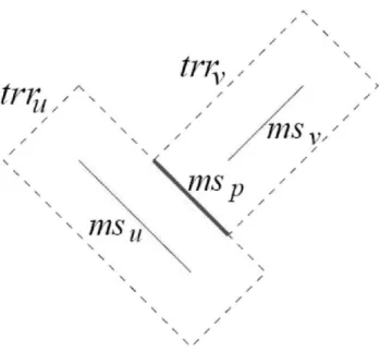
Figure 2.1: Construction of a merging segment ms(p) = trru∩ trrv

Manhattan arc at the center of a RTT is called the core. The radius of a TRR is the Manhattan distance between its core and its boundary. It is shown in Figure 2.1 that ms(p) = trru ∩ trrv , where trru is the TRR with core msu, and radius

|eu| and trrv is the TRR with core msv and radius |eu|. The radius |eu| and |ev| are computed by the delay model described in Chapter 2.2 and Manhattan distance between u and v.

2.2

Delay Model

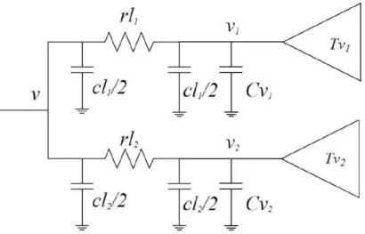
We assume that a clock tree is a binary tree in which the root is the clock source and the leaves are clock pins (flip-flops). Delay model is used in computing the signal propagation delay of the clock tree. Figure 2.2 shows the delay model of zero-skew merging (no buffers). Let tv denote the delay from v to leaf of subtree Tv . Then

Figure 2.2: Zero-skew merging with no buffers. v1 and v2 are subtrees of parent

node v

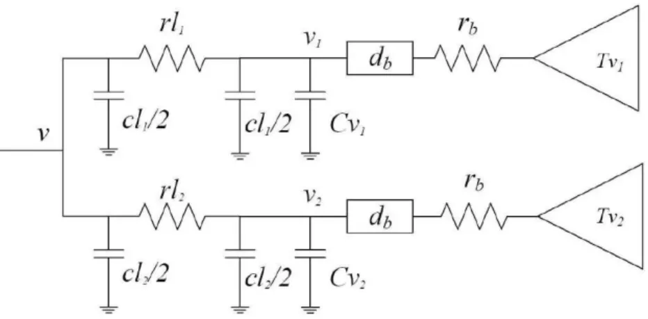
Figure 2.4: Zero-skew merging with buffers. v1 and v2 are subtrees of parent node

v

where l1(l2) is the wire length from v to v1(v2) , and r and c are per unit resistance

and per unit capacity of the routing wire. Cv is the downstream capacitance of v shown below:

Cv = Cv1+ Cv2

Buffer insertion is another important part in clock tree design. The model of the buffer is shown in Figure 2.3. cb , db , and rb are the input capacity, output resister, and delay of buffer. Figure 2.4 shows the delay model of zero-skew merging with buffers inserted. The tv and Cv are updated by following:

tvi = db + rb× Cvi+ t

0

vi(i = 1, 2), Cv = Cb+ Cb

2.3

Problem Formulation

We assume that the clock tree is routed by 2-layer routing (vertical and horizontal), but it can be extended to mutilayer. The problem we will solve is formally stated as follows.

Given a set of clock pins S = {s1, s2, ..., sn} and a clock root vr. A clock tree is

defined by a tree rooted by vr and the sinks are S. X range(Y range) are defined

as the maximum difference length of vertical( horizontal) metal between source and sinks. We want to construct a zero-skew clock tree T rooted at vr with clock sinks

as leaf nodes such that the X range and Y range between source and sinks are min-imized.

Chapter 3

Metal-balance Algorithm

In this chapter, we briefly describe our algorithm, which is based on DME algorithm. In order to make metal balance clock tree, we modify the DME algorithm [1] to fit our requirement. The details of these modifications are shown in the following subsections. Section 3.1 is to choose the minimum cost for clock topology. Section 3.2 is our metal balance algorithm. After Section 3.1 and 3.2, an metal-balance unbuffered clock tree is builded. Section 3.3 is to build an metal-balance buffered clock tree.

3.1

Metal Balance Aware Clustering

The influence of clock tree topology is significant. Because we do not have the topol-ogy of clock tree, we have to cluster the nodes to construct the binary clock tree. Furthermore, we use the simple clustering algorithm to form our clock tree topol-ogy. For traditional matching-based methodology [20] [21], a geometric matching of 2N segments or sinks cluster into N groups between segment, with no two of the N group sharing the same segments. [22] proposed NS (Nearest-neighbor selection) algorithm. We modify the NS algorithm to satisfy our requirement.

the nearest neighbor pair v1 and v2 from K, calculates a segment for v from v1 and

v2 using the zero-skew merge, and put the segment into K, then, delete v1 and v2

from K. After n-1 operation, K has only one element that is the segment for all the sinks.

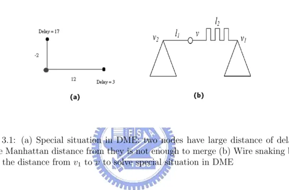
Figure 3.1: (a) Special situation in DME: two nodes have large distance of delay and the Manhattan distance from they is not enough to merge (b) Wire snaking by adding the distance from v1 to v to solve special situation in DME

However, choosing the nearest neighbor pair will cause one special situation. When the delay difference of two merging segments is too large, there is not enough Man-hattan distance to make the delays from merging point to two segments are the same. For example, in Figure 3.1(a) , the two points have delay 17 and delay 3 to their sinks. The Manhattan distance between them is 10. After DME algorithm, we get that we need -2 and 12 wirelength from merging point to two points. This is impossible. In general, we solve this by snaking in Figure 3.1(b), but snaking is not good for clock tree. Hence, we should avoid special situations. The way is to choose a merging point by less delay differences and Manhattan deistance among all merging segments. Merging cost is well-estimated by the following formulation.

Cost(i, j) = _distDIST AN CE(i,j) + |Delayi−Delayj|

Cost(i,j) is the merging cost of the merging segment MSi and merging segment MSj.

Distance(i, j) is the Manhattan distance of MSi and MSj. Delayi means that the delay time from MSi to the sinks. disthalf −perimeter is the half perimeter of the chip core, and the delayhalf −perimeter is the RC delay of the half perimeter of the chip core,delayhalf −perimeter = (r0 × disthalf −perimeter) × (c0 × disthalf −perimeter). We nor-malize the distance and delay. So that, we can add these two factors to estimate the cost. The minimum cost pair has highest priority to be merged. By the considera-tion of delay and distance, we can avoid the merging of unbalance merging segments.

This cost function has another advantage for metal balance. When pair nodes have similar capacity load, their merging segment can make two nodes have less difference metal length from sinks. Hence, by using this cost function, we can get more balanced clock tree topology.

3.2

Metal-balance Algorithm Based on DME

In the top-down phase of DME, DME resolves the exact locations of all internal nodes in ZST. The exact locations are always the end points of merging segments because DME tries to find the shortest path. However, the end points offten have the maximum wirelength difference from end points to their children. Therefore, DME is not suit to build metal balance clock tree.

Our algorithm is based on DME [1]. The primary differences are our algorithm combines two phases, button-up and top-down, into one phase. Our goal is to min-imum the maxmin-imum metal length difference between clock source and clock sinks. In Section 2.3, we assume that clock tree is routed by two layers (horizontal and vertical). Hence, we use 4x (4y) to represent the X ragne(Y range) difference in our work.

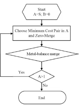
Figure 3.2: Flow of non-buffer Metal-balance clock tree algorithm

A flow of the algorithm is illustrated in Figure 3.2. The algorithm maintains two sets, A and B. A is a set of nonmerged nodes and is initialized to a set of sinks. B is a set of merged nodes and is initialized as an empty set. The flow first clusters the sinks ( or merging points) of A. We sort the cost of each pair of the merging segments. The minimum cost pair is selected from A by our clustering algorithm in Section 3.1.

Then, we merge two nodes. In A and B sets, node n saves four data, (max 4

Xn, min4Xn, max4Yn, min4Yn), which are initialized (0,0,0,0). max4Xn(min4

Xn) is the maximum (minimum) 4x between node n to its sinks. max4Yn(min4Yn ) is the maximum (minimum) 4y. Figure 3.4 shows the result when merging two nodes v1 and v2.(Xv, Yv), (Xv1, Yv1), (Xv2, Yv2) are the location of node v, v1, and

Figure 3.3: A result of Metal-balance merge. v1 to v2 are the children of v.

Lv1,Lv2,and Lv are data for metal balance.

v2. X1(Y1) and X2(Y2) mean the difference of wirelength in metal X(Y). Node v is

one point in merging segment of v1 and v2 and the four data of all points in segment can be counted by the same way. Then, we choose the point which has the minimum metal balance cost for merging point. The metal balance cost is as following.

Costf unction = α 4 x0+ β 4 y0

α and β are user defined variables. If we only want to balance the horizontal metal,

we can choose α =1 and β =0. 4x0 and 4y0 is counted by

M x0 = max M X − min M X

M y0 = max M Y − min M Y

After choosing the merging point v, we use v to replace v1 and v2 in A. We repeat the flow until the member in A is one.

Figure 3.4: A example of Metal-balance merge. v1 and v2 are the children of v.

LV1, LV2, and LV are the metal balance data of v1, v2, and v.

Figure 3.4 shows an example of the metal balance merge. The saved data in node v1 is (2,1,2,1) and in node u2 is (2,0,2,0). Then after DME, we have five node on merging segment. Take v for example,after our flow, the four data of v is (7,4,5,2). The cost is 7-4+5-2=6. Then we calculate costs of other points. Finally, we choose the minimum cost point for our merging point.

3.3

Buffered Metal Balance Clock Tree

In order to verify that metal balance algorithm in buffered clock tree can still tol-erate manufacturing process, we modify the algorithm in [19] for building buffered metal balance clock tree.

In a practical solution of buffer insertion, it is usually desired that all root-to-leaf paths have the same number of buffer stages. It can make the impact of process variation on the skew of a clock net minimize if there is a change in buffer delay due to process variation. This is because the increment of decrement of phase delay

Figure 3.5: Level-by-level insert buffers method in binary tree

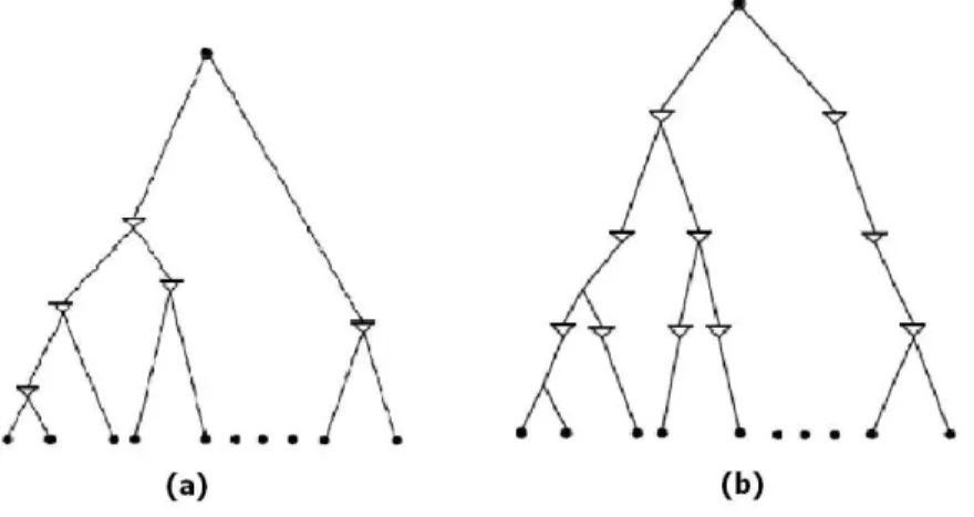
is the same for all paths. Level-by-level method is usually used in many works. It is shown Figure 3.5. However, this method works well when the tree topology is full binary tree where all sinks have same number of levels. If the clock tree is not full binary tree in Figure 3.6(a), the number of buffers from source to sinks are not the same. Hence, balanced buffer insertion method is preferred in [19]. This method starts with an equal path-length clock tree T. Then, they insert buffers at the same distance from clock source. Then, even the tree does not have clear level, this method can still guarantee that there are same number buffer from source to sinks. Figure 3.6(b) is the balanced buffer insertion method. Our paper is suited the balanced buffer insertion method due to our clustering.

Our process of building buffered metal balance clock tree has three steps. First, we build a metal balance unbuffered clock tree. The primary difference is the clock tree must be an equal path-length clock tree. We use Manhattan distance to replace delay for merging. If there is the same delay from source to sink, there is the same

distance from source to sinks. Second, we find the buffer insert location. The buffer location is as follows:

buf f erlocation = L/(n + 1)

L is the path distance from clock source to sink. n is initialized 1. Thirdly, we

calculate the skew from clock source to sinks and check timing constrain is satisfied. If the timing constrain is not satisfied, we add n by 1 and repeat step2 until the timing constrain is satisfied. Finally, we get a buffered metal balance clock tree.

Figure 3.6: (a) Level-by-level method in non full binary clock tree (b) The balance buffer insertion method in non full binary clock tree

Chapter 4

Experiment Results

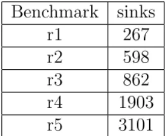
We have implemented our approach in the C++ programming language and tested it on AMD Opteron (tm) 2.8G with 2.0GB memory. We use UMC 90nm standard cell library for conventional buffers. The benchmark circuits are r1-r5 downloaded from the GSRC Bookshelf (http://vlsicad.ucsd.edu/GSRC/bookshelf/Slots/BST/). Table 4.1 shows the number of sinks in benchmark r1-r5.

Table 4.2 shows the 4x and 4y of DME and our metal-balance. Fifth and sixth columns are the improvement between ours and DME. We can find that ours 4x and 4y is less than DME 20% to 70%. Hence, our research can make the clock tree more balance.

In order to simulate the effect of the manufacturing variations, we add two pa-rameters in delay model:

r(αLx+ βLy)(c(αLx₂+βLy) + Cv1) + tv1

The primary difference is that we use (αLx+ βLy) to replace the distance l. α and

β are user defined. Lx and Ly are the length of horizontal and vertical. The result is showed in Table 4.3. It compares the results of DME and our metal-balance algo-rithm in nonbuffered clock tree. The first column shows the wirelength of DME and

we normalize the DME wirelength to 1. The third column shows the ratio of ours to DME. The wirelength of ours is more than DME 1% to 7%.This is because that DME is an algorithm that tries to find the minimum wirelength. The second and forth columns are the skew of DME and ours based on the new delay model where

α = 1.1 and β = 0.9. In fifth column, it shows that our algorithm can reduce the

skew under process violation. Therefore, this is a trade off between wirelength and process violation.

Table 4.4 shows the result of DME and ours in buffered clock tree. The first and second columns are the skew of DME and ours. Because buffer insert can reduce the arrival time, we can see that the skew difference between DME and ours is less than table 4.2. However,we can still get from third column that our skew is still less than DME.

4.1

Discussion

In the top-down phase of DME [1], DME resolves the exact locations of all internal nodes in ZST. The exact locations are always the end points of merging segments because DME tries to find the shortest path. However, the end points often have the maximum wirelength difference from end points to their children. In [2]- [9], they improve the bottom-up phase of DME, but their top-down phase is the same as in DME. They all try to find the shortest path. Hence, they can not balance the wirelength of every metal and skew will be effected easily by manufacturing process.

Table 4.1: The number of sinks in benchmark r1-r5. The benchmark circuits are downloaded from the GSRC Bookshelf.

Benchmark sinks r1 267 r2 598 r3 862 r4 1903 r5 3101

Table 4.2: The table shows the comparison of wirelength difference of horizontal and vertical metal by using DME and metal balance(MB). The results present advantages in balance. The 4x of MB is average 36% less than DME. The 4y of MB is average 30% less than DME.

DME 4x DME 4y MB 4x MB 4y 4x improve 4y improve r1 29093.5 29503.2 20561.8 22033.4 29% 25% r2 54878.79 45205.6 35044.7 32840.2 36% 27% r3 57852.77 57337.6 43300.1 30522.1 25% 47% r4 58434.2 68738.6 46557.4 52534.2 20% 24% r5 126556.1 62453.4 32376.2 46274.3 74% 26%

Table 4.3: The wirelength and skew comparison between DME and metal bal-ance(MB) in unbuffered clock tree under manufacturing process. The results present advantages in skew. MB skew is average 60% less than DME. However, MB wire-length is average 4% more than DME.

DME WL DME skew (ps) MB WL MB skew (ps) skew improve r1 1 17.2 1.001 4.4 74% r2 1 45 1.048 29 36% r3 1 113 1.045 37 67% r4 1 310 1.069 97 69% r5 1 650 1.035 290 55%

Table 4.4: The skew comparison between DME and metal balance(MB) in buffered clock tree under manufacturing process. The results present advantages in skew. MB skew is average 37% less than DME.

DME skew (ps) MB (ps) Skew improve r1 5.5637 3.5234 37% r2 5.87 1.5 74% r3 21.602 18.957 12% r4 1.34 1.057 21% r5 15 8.384 44%

Chapter 5

Conclusion and Future Work

In this thesis, we propose a methodology to make a metal-balance clock tree. In non-buffered clock tree, our method guarantees that more tolerance of process vari-ation. In buffered clock tree, our method can reduce skew dues to process varivari-ation. According to the results, we believe that our algorithm can be applied to most de-signs to construct metal-balance clock tree.

In future works, we plan to improve three problems. The first is the wirelength. Less wirelength can reduce the power of clock tree. Hence, how to make our clock has less wirelength is important. The second is counting time. Our method costs much time to find the best metal-balance solution. The third is locality problem. When the cell becomes bigger, only to balance the wirelength of each metal layer may not be enough to make the clock tree more tolerance process variation. In future, we will try to solve these three problems.

Bibliography

[1] T.-H. Chao, Y.-C. Hsu, and J.-M. Ho, ”Zero Skew Clock Net Routing,” in

Proc. IEEE/ACM Design Automation Conference, pp. 518-523, 1992.

[2] I-Min Liu, T.-Li Chou Adnan Aziz, and D.F. wong, ”Zero-skew Clock Tree Construction by Simultaneous Routing, Wire Sizing and Buffer Insertion,” in

Proc. International Symposium on Physical Design, pp. 33-38, 2000.

[3] D. J.-H. Huang, A. B. Kahng, and C.-W. A. Tsao, ”On the Bounded-Skew Clock and Steiner Routing Problems,” in Proc. IEEE/ACM Design Automation

Conference, pp. 508-513, June 1995.

[4] J. Cong, A. B. Kahng, C.-K. Koh, and C.-W. A. Tsao, ”Bounded-Skew Clock and Steiner Routing Under Elmore Delay,” in Proc. IEEE/ACM International

Conference on Computer-Aided Design, pp. 66-71, 1995.

[5] J. Cong, A. B. Kahng, C.-K. Koh, and C.-W. A. Tsao, ”Bounded-Skew Clock and Steiner Routing,” in ACM Trans. on Design Automation of Electronic

Systems, Vol. 4, No. 1, January, 1999.

[6] U. Padmanabhan, J. M. Wang, and J.Hu, ”Statistical Clock Tree Routing for Fobustness to Process Variations,” in Proc. International Symposium on

[7] M. Cho, S. Ahmed, and D. Z. Pan, ”Taco: Temperature Aware Clock-tree Optimization,” in Proc. Int. Conf. on Computer Aided Design, pp. 582-587, 2005.

[8] B. Lu, J. Hu, G. Ellis, and H.Su, ”Process Variation Aware Clock Tree Rout-ing,” in Proc. International Symposium on Physical Design, 2003, pp. 174-181. [9] J. Miinz, X. Zhao, and S. K. Lim, “Buffered Clock Tree Synthesis for 3D ICs Under Thermal Variations,” in Proc. Asia and South Pacific Design Automation

Conference, pp. 504-509, 2008.

[10] A. Rajaram, J. Hu, and R. Mahapatra, “Reducing Clock Skew Variability Via Cross Links,” in Proc. IEEE/ACM Design Automation Conference, pp. 18-23, 2004.

[11] W.-C. D. Lam, J. Jam, C.-K. Koh, V. Balakrishnan, and Y. Chen, “Statistical Based Link Insertion for Robust Clock Network Design,” in Proc. IEEE/ACM

International Conference on Computer-Aided Design, pp. 588-591, 2005.

[12] A. Rajaram and D. Z. Pan, “Variation Tolerant Buffered Clock Network Syn-thesis with Cross Links,” in Proc. International Symposium on Physical Design, pp. 157-164, 2006.

[13] G. Venkataraman, N. Jayakumar, J. Hu, P. Li, S. Khatri, A. Rajaram, P. McGuinness, and C. Alpert, “Practical Techniques to Reduce Skew and Its Variations in Buffered Clock Networks,” in Proc. IEEE/ACM International

Conference on Computer-Aided Design, pp. 592-596, 2005.

[14] M. Mori, H. Chen, B. Yao, and C.-K Cheng, “A Multiple Level Network Approach For Clock Skew Minimization with Process Variations,” in Proc. Asia

[15] A. Fajaram, D. Z. Pan, and J. Hu, “Improved Algorithms for Link-Based Non-Tree Clock Networks for Skew Variability Reduction,” in Proc. International

Symposium on Physical Design, 2005, pp. 592-596.

[16] A. Rajaram and D. Z. Pan, “Fast Incremental Link Insertion in Clock Networks for Skew Variability Reduction,” in Proc. International Symposium on Quality

Electronic Design, pp. 79-84, 2006.

[17] J.-S. Yang, A. Gajaram, N. Shi, J.Chen, and D. Z. Pan, “Sensitivity Based Link Insertion for Variation Tolerant Clock Network Synthesis,” in Proc.

Inter-national Symposium on Quality Electronic Design, pp. 398-403, 2007.

[18] G. Venkataraman, Z. Feng, J. Hu, and P. Li, “Combinatorial Algorithms for Fast Clock Mesh Optimization,” in Proc. IEEE/ACM International Conference

on Computer-Aided Design, pp. 563-567, 2006.

[19] J. G. Xi and Wayne W.-M. Dai, “Buffer Insertion and Sizing Under Process Variations for Low Power Clock Distribution,” in Proc. IEEE/ACM Design

Automation Conference, pp. 491-496, 1995.

[20] A. B. Kahng, J. Cong, and G. Robins, “Matching-based Methods for High Performance Clock Routing,” in IEEE Trans. on Computer-Aided Desigh of

Integrated Circuits and Systems, Vol. 12, No. 8, August, 1993.

[21] J. Pangjun and S. S. Sapatnekar, “Low-power Clock Distribution Using Mul-tiple Voltages and Reduced Swings,” in IEEE Trans. on Very Large Scale

In-tegration Systems, Vol. 10, No. 3, June, 2002.

[22] M. Edahiro, “A Clustering-based Optimization Algorithm in Zero-skew Rout-ings,” in Proc. IEEE/ACM Design Automation Conference, pp. 612-616, 1993.