使用數位架構的正交分頻多工系統關於峰均比之研究

全文

(1)國立交通大學電機與控制工程學系碩士論文. 使用數位架構的正交分頻多工系統關於峰均比之研究. A Study of PAPR for OFDM System Using a Digital Framework. 研究生：. 劉翔澤. 指導教授：. 林源倍. 博士. 中華民國九十七年九月.

(2) 使用數位架構的正交分頻多工系統關於峰均比之研究 A Study of PAPR for OFDM Systems Using a Digital Framework 研究生 : 劉翔澤. Student : Shiang-Tze Liou. 指導教授 : 林源倍. 博士. Advisor : Dr. Yuan-Pei Lin. 國立交通大學電機與控制工程學系碩士論文. A Thesis Submitted to Institute of Electrical and Control Engineering College of Electrical Engineering National Chiao Tung University In Partial Fulfillment of the Requirements In Electrical and Control Engineering September 2008 Hsinchu, Taiwan, Republic of China. 中華民國九十七年九月.

(3) 使用數位架構的正交分頻多工系統關於峰均比之研究. 研究生 : 劉翔澤指導教授 : 林源倍博士. 國立交通大學電機與控制工程學系. 碩士班. 中文摘要傳送訊號的峰均比( peak-to-average power ratio, PAPR )在正交分頻多工系統 ( OFDM system )中是很重要的討論議題。這個性質通常使用類比架構的正交分頻多工系統來做分析。為了要得到傳輸端輸出訊號的峰均比，我們通常都會對連續時間的訊號作過度取樣( oversampling )的動作。至於，過度取樣的取樣點多寡則視所需要的 PAPR 值決定。早期的研究都是使用過度取樣因子( oversampling factor )為 4 來估計實際上的峰均比。現在實際上所使用的正交分頻多工系統是使用不可逆的離散傅立葉轉換矩陣 ( IDFT matrix ) 和數位類比轉換器 ( digital-to-analog converter )來構成傳輸端。使用離散傅立葉轉換矩陣( DFT matrix ) 和類比數位轉換器( analog-to-digital )來組成接收端。在這篇論文裡面，我們會使用數位架構的正交分頻多工系統來考慮傳輸端輸出訊號的峰均比問題。模擬的結果顯示出過度取樣因子也許需要大於 4 來獲得比較接近連續時間的峰均比。除此之外，也可以發現嵌置在數位類比轉換器中的傳輸濾波器，以及嵌置在類比數位轉換器中的接收濾波器都會影響峰均比、位元錯誤率( bit error rate )、以及所需的過度取樣因子。.

(4) 誌謝從對通訊和寫程式幾乎沒有概念，到現在開始有一點點粗淺的了解，這兩年對我而言是意義重大的里程。非常感謝指導教授. 林源倍. 老師在過程中，不厭其煩地細心教導，也給我很多的時間和空間去學習。不論是專業領域或是待人處事上，老師都給予我很大的幫助，真的很感謝老師! 同時也感謝口試委員鄭木火教授和蔡尚澕教授百忙之中給予我指導和建議。感謝實驗室的大家: 建樟學長、鈞麟學長、Jeff學長、素卿、芳儀、士軒、懿德在這兩年的學習過程給我的幫助。要特別感謝電信所的千雅學姊和汀華學姊，當我在學習上遇到瓶頸，或是心情鬱悶時，給我的幫助和鼓勵。也謝謝福智團體的老師、同學和師兄姊們的陪伴和幫助，因為有你們讓我的生活更充實。感謝我的好朋友駿璿、香璽、旭富在我最無助的這段時間給我的幫助和支持。感謝我最親愛的家人:爸媽、阿姨、博華、瑋慈、佳勳，以及詔聘，謝謝你們給我的支持、鼓勵，和陪伴。你們是支持著我繼續努力下去的動力。也因為有你們我才能在這過程中學習、成長。感謝這一路上和我相遇的人們! 因為有你們，我才得以成為現在的我，謝謝你們!.

(5) A Study of PAPR for OFDM Systems Using a Digital Framework. Student : Shiang-Tze Liou. Advisor : Yuan-Pei Lin. Department of Electrical and Control Engineering National Chiao Tung University. Abstract The peak to average power ratio (PAPR) is an important issue in OFDM systems. The quantity is typically analyzed using an analog representation of the OFDM transmitter. To obtain an estimate of the PAPR of transmitter output, the continuous-time transmitted signal is usually oversampled, based on which PAPR is computed. It has been shown earlier that an oversampling factor of 4 gives a good estimate of the actual PAPR. Modern OFDM systems are invariably implemented using an inverse discrete Fourier transform and a digital-to-analog converter for the transmitter, and a discrete Fourier transform and an analog-to-digital converter for the receiver. In this thesis, we consider the PAPR of OFDM transmitter outputs using the digital framework. The simulation results show that an oversampling factor of more than 4 may be needed to obtain a good estimate of the continuous-time PAPR value. Furthermore, the transmitting filter embedded in the digital-to-analog converter and the receiving filter embedded in the analog-to-digital converter also affect PAPR, bit error rate, and the required oversampling factor.. i.

(6) Contents English Abstract. i. Contents. ii. List of Figures. iv. List of Tables. vii. 1 Introduction. 1. 1.1. Outline . . . . . . . . . . . . . . . . . . . . . . . . . . . . . . . . . . . . .. 4. 1.2. Notations . . . . . . . . . . . . . . . . . . . . . . . . . . . . . . . . . . .. 4. 2 Review of OFDM System. 6. 2.1. Analog Framework OFDM System Model . . . . . . . . . . . . . . . . . .. 6. 2.2. Digital Framework OFDM System Model . . . . . . . . . . . . . . . . . .. 8. 2.3. Analog Framework System Model Versus Digital Framework System Model. 9. 3 System Model. 13. 3.1. Peak to Average Power Ratio (PAPR) . . . . . . . . . . . . . . . . . . .. 13. 3.2. Continuous-Time Fading Channel . . . . . . . . . . . . . . . . . . . . . .. 18. 3.3. Equivalent Discrete-Time Channel . . . . . . . . . . . . . . . . . . . . . .. 19. 3.4. Noise Generation . . . . . . . . . . . . . . . . . . . . . . . . . . . . . . .. 22. 3.5. Bit Error Rate. 24. . . . . . . . . . . . . . . . . . . . . . . . . . . . . . . . .. ii.

(7) 4 Numerical Simulation 4.1. 4.2. 4.3. 4.4. 4.5. 27. Case 1 . . . . . . . . . . . . . . . . . . . . . . . . . . . . . . . . . . . . .. 29. 4.1.1. Peak to Average Power Ratio . . . . . . . . . . . . . . . . . . . .. 31. 4.1.2. Bit Error Rate . . . . . . . . . . . . . . . . . . . . . . . . . . . .. 31. Case 2 . . . . . . . . . . . . . . . . . . . . . . . . . . . . . . . . . . . . .. 37. 4.2.1. Peak to Average Power Ratio . . . . . . . . . . . . . . . . . . . .. 37. 4.2.2. Bit Error Rate . . . . . . . . . . . . . . . . . . . . . . . . . . . .. 39. Case 3 . . . . . . . . . . . . . . . . . . . . . . . . . . . . . . . . . . . . .. 44. 4.3.1. Peak to Average Power Ratio . . . . . . . . . . . . . . . . . . . .. 46. 4.3.2. Bit Error Rate . . . . . . . . . . . . . . . . . . . . . . . . . . . .. 47. Case 4 . . . . . . . . . . . . . . . . . . . . . . . . . . . . . . . . . . . . .. 51. 4.4.1. Peak to Average Power Ratio . . . . . . . . . . . . . . . . . . . .. 53. 4.4.2. Bit Error Rate . . . . . . . . . . . . . . . . . . . . . . . . . . . .. 53. Summary . . . . . . . . . . . . . . . . . . . . . . . . . . . . . . . . . . .. 59. 5 Conclusion. 62. Bibliography. 64. iii.

(8) List of Figures 2.1. The analog framework baseband model of OFDM system. . . . . . . . . .. 7. 2.2. The digital framework baseband model of OFDM system. . . . . . . . . .. 9. 2.3. The transmitter of the digital framework modl of the OFDM system. . .. 10. 3.1. The Process of producing xL (n) . . . . . . . . . . . . . . . . . . . . . . .. 16. 3.2. The part from x(n) to r(n) . . . . . . . . . . . . . . . . . . . . . . . . . .. 19. 3.3. The equivalent discrete-time channel . . . . . . . . . . . . . . . . . . . .. 20. 3.4. Channel noise of the digital framework OFDM system model . . . . . . .. 22. 3.5. The equivalent discrete-time channel . . . . . . . . . . . . . . . . . . . .. 22. 3.6. The equivalent discrete-time channel. . . . . . . . . . . . . . . . . . . . .. 25. 4.1. The transmit spectrum mask under IEEE 802.11a . . . . . . . . . . . . .. 28. 4.2. The form of inputs for IFFT matrix . . . . . . . . . . . . . . . . . . . . .. 28. 4.3. (a)The magnitude responses (b)The impulse responses of elliptic analog filters with distinct stopband edges. . . . . . . . . . . . . . . . . . . . . .. 4.4. 30. The PAPR curves of elliptic analog filters with distinct stopband edges ws . (a) ws is 0.7 fs. (b)ws is 1.0 fs. (c) ws is 1.2 fs. (d) The PAPR curves of these three filters and the oversampling factor is 32. . . . . . . . . . .. 4.5. (a) The impulse response (b) The magnitude response (c) BER performance of c1 (n). 4.6. 33. . . . . . . . . . . . . . . . . . . . . . . . . . . . . . . . .. 35. (a) The impulse response (b) The magnitude response (c) BER performance of c2 (n). . . . . . . . . . . . . . . . . . . . . . . . . . . . . . . . . iv. 36.

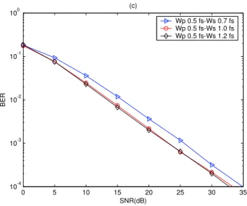
(9) 4.7. (a)The magnitude responses (b)The impulse responses of elliptic analog filters with distinct transition band bandwidths which center at 1.0 fs. . .. 4.8. 38. The PAPR curves of elliptic analog filters with distinct transition band bandwidths. (a) wp is 0.2 fs and ws is 0.8 fs. (b)wp is 0.5 fs and ws is 1.5 fs. (c) wp is 0.8 fs and ws is 1.2 fs. (d) The PAPR curves of these three filters and the oversampling factor is 32. . . . . . . . . . . . . . . . . . .. 4.9. 41. (a) The impulse response (b) The magnitude response (c) BER performance of c3 (n). . . . . . . . . . . . . . . . . . . . . . . . . . . . . . . . .. 42. 4.10 (a) The impulse response (b) The magnitude response (c) BER performance of c4 (n). . . . . . . . . . . . . . . . . . . . . . . . . . . . . . . . .. 44. 4.11 (a)The magnitude responses (b)The impulse responses of elliptic analog filters with distinct passband edges. . . . . . . . . . . . . . . . . . . . . .. 45. 4.12 The PAPR curves of elliptic analog filters with distinct passband edges wp . (a) wp is 0.2 fs. (b)wp is 0.5 fs. (c) wp is 0.8 fs. (d) The PAPR curves of these three filters and the oversampling factor is 32. . . . . . . . . . .. 48. 4.13 (a) The impulse response (b) The magnitude response (c) BER performance of c5 (n). . . . . . . . . . . . . . . . . . . . . . . . . . . . . . . . .. 49. 4.14 (a) The impulse response (b) The magnitude response (c) BER performance of c6 (n). . . . . . . . . . . . . . . . . . . . . . . . . . . . . . . . .. 51. 4.15 (a)The magnitude responses (b)The impulse responses of elliptic analog filters with the same transition band bandwidth. . . . . . . . . . . . . . .. 52. 4.16 The PAPR curves of elliptic analog filters with the same transition band bandwidth and distinct useful band bandwidths. (a)wp is 0.2 fs and ws is 0.9 fs. (b)wp is 0.5 fs and ws is 1.2 fs. (c) wp is 0.8 fs and ws is 1.5 fs. (d) The PAPR curves of these three filters and the oversampling factor is 32.. 55. 4.17 (a) The impulse response (b) The magnitude response (c) BER performance of c7 (n). . . . . . . . . . . . . . . . . . . . . . . . . . . . . . . . .. v. 57.

(10) 4.18 (a) The impulse response (b) The magnitude response (c) BER performance of c8 (n). . . . . . . . . . . . . . . . . . . . . . . . . . . . . . . . .. vi. 58.

(11) List of Tables 4.1. Parameters of digital framework OFDM system . . . . . . . . . . . . . .. 29. 4.2. Parameters of case 1 . . . . . . . . . . . . . . . . . . . . . . . . . . . . .. 29. 4.3. Parameters of case 2 . . . . . . . . . . . . . . . . . . . . . . . . . . . . .. 37. 4.4. Parameters of case 3 . . . . . . . . . . . . . . . . . . . . . . . . . . . . .. 45. 4.5. Parameters of case 4 . . . . . . . . . . . . . . . . . . . . . . . . . . . . .. 52. 4.6. γ of case 1 . . . . . . . . . . . . . . . . . . . . . . . . . . . . . . . . . . .. 60. 4.7. γ of case 2 . . . . . . . . . . . . . . . . . . . . . . . . . . . . . . . . . . .. 60. 4.8. γ of case 3 . . . . . . . . . . . . . . . . . . . . . . . . . . . . . . . . . . .. 60. 4.9. γ of case 4 . . . . . . . . . . . . . . . . . . . . . . . . . . . . . . . . . . .. 61. vii.

(12) Chapter 1 Introduction The present communications systems are primarily designed for one specific application, such as speech on mobile telephone or high-rate data in wireless local area networks (LANs). The orthogonal frequency division modulation (OFDM)[1][2] is the most popular modulation operated on the high-rate data transmission system.There are many international standard established for using OFDM system on high-rate data wireless communication, such as IEEE 802.11a and IEEE802.11m. The basic principle of OFDM is to split a high-rate data stream into a number of lower rate data streams that are transmitted simultaneously over a number of subcarriers. There are two kinds of the OFDM system models. One is analog framework OFDM system model, and the other is digital framework OFDM system model. The main difference between these two kinds of OFDM system models is described as following. Based on the analog framework OFDM system model, the data stream passes through a shaping pulse filter to produce the continuous-time signal at the transmitter site. The transmitter of the analog representation framework OFDM system model works at continuous-time. For digital representation framework OFDM system model, the continuous-time signal is produced by passing data stream through a inverse discrete Fourier transform (IDFT) matrix and a digital-to-analog (D/C) converter. Not the same as the transmitter of analog representation framework OFDM system model, the. 1.

(13) transmitter is operated digitally. Because of the convenience, many existing results on the analysis of OFDM system [3], e.g. PAPR problem, the spectral roll-off of the outputs of OFDM transmitter, the effect of carrier frequency offset, and crest factor of the transmitter outputs, are based on the analog representation framework of the OFDM system. In fact, the OFDM system is implemented digitally. We know that the outputs of the transmitter of these two models have considerable difference [4]. Therefore, analyzing the OFDM system using the digital framework OFDM system model is more useful than the analog one. Different from the common analyzing model, in this thesis, we will take digital framework OFDM system model to analyze some behaviors of OFDM system. In addition to the system model, we know that when we discuss the digital representation framework OFDM system model, we usually ignore the effect of the transmitting pulse and receiving pulse and take them as ideal lowpass filters. Otherwise, the transmitting pulse and receiving pulse are not ideal lowpass filters in practice. Under the restriction of the IEEE 802.11a standard, we try to give four realizable filter design cases to design the transmitting and receiving pulses. Then do some simulations to observe some behaviors of digital representation framework OFDM system model. When the digital representation framework OFDM system model is implemented, the transmitted continuous-time signals needs passing through the power amplifier between the D/C converter and the physical channel. Because we expect the power amplifier operated on the high efficiency linear region [5] that often operating at the average power levels, the peak power of transmitted signal does not exceed the average power too much. Therefore, the peak to average power ratio (PAPR) value is needed to know for system designer. The peak to average power ratio is high when the numbers of the subcarriers is large. The OFDM system uses a lot of subcarriers, e.g. 2048, that would result in high PAPR. Owing to high PAPR, the PAPR problem becomes the popular issue for OFDM system. Therefore, there are many PAPR reduction methods proposed. 2.

(14) to solve the PAPR problem, for example, clipping [6], selective mapping (SLM) [7], and partial transmit sequence (PTS) [8]. The PAPR performance is the main point that we want to observe in this thesis. Usually, we compute the PAPR value based on the analog representation framework system model. The oversampling factor is 4 for computing the continuous-time PAPR value. In this thesis, we use the digital representation framework OFDM system model and realizable transmitting and receiving pulses to simulate the PAPR performance in practice. We also observe if the oversampling factor used 4 enough for analyzing the PAPR problem. The bit error rate (BER) performance is observed, too. There are two kinds of environments that we use to discuss the BER performance. The continuous-time channel is set for additive white Gaussian noise (AWGN) and Rayleigh fading respectively for simulating. Observing the simulation results in this thesis, we can see that some properties of PAPR are different from the existing results, such as the oversampling factor may more than 4 to get closer the continuous-time PAPR value. We can also find out that the PAPR value is changed with the different transmitting pulse designs. The better PAPR performance occurs when the useful band bandwidth of the transmitting reconstruction filter is smaller. The transmitting pulse design could be use to reduce the PAPR. The BER performance is affected by the transmitting and receiving pulses, too. The wider useful band bandwidth results in larger equivalent discrete-time channel response, and that makes the BER performance better. From this thesis, we can conclude that the transmitting pulse and receiving pulse indeed affect some behaviors of OFDM system, such as PAPR and BER performance. The filter design might a trade-off problem when we want to have both better PAPR and BER performance, which design is the best choice just depends on what advantage we request for.. 3.

(15) 1.1. Outline. 1. Chapter 1: Introduction. 2. Chapter 2: We will introduce two kinds of OFDM system models that are analog framework and digital framework system models. The analog framework system model is an ideal system model, and we use such a system model to analysis the behavior of OFDM system. But we use the digital framework system model in practice. In this chapter, we also show the difference between these two system models. 3. Chapter 3: We will introduce the definition of peak to average power ratio (PAPR) and bit error rate (BER). The Continuous-time fading channel [fad1] [fad2] and its equivalent discrete-time channel would be mentioned, too. In this chapter, we also explain how to generate the discrete-time noise for our simulation. 4. Chapter 4: In this chapter, we use five cases to simulate the behavior of OFDM system based on digital framework system model. To observe what difference between analog framework and digital framework OFDM system model for PAPR performance and BER performance. 5. Chapter 5: Conclusion is given in this chapter.. 1.2. Notations. 1. Bold face upper case letters represent matrices, and bold face lower case letters represent vectors. AT denotes transpose of A, and A† denotes conjugate transpose of A. 4.

(16) 2. The function E[x] denotes the average value or expected value of x. 3. ∗ denotes the linear convolution. 4. M is the DFT size, ν is the CP length, N is the numbers of subcarriers, Ts is the sampling period, and m is the taps of the continuous-time channel ca (t). 5. The notation W notes the normalized M × M DFT matrix, it is given by [W]kn =. 2π √1 ej M kn , M. where 0 ≤ k, n ≤ M − 1.. 6. wp is the passband edge, ws is the stopband edge, Rp is the passband ripple, Rs is the stopband attenuation, and fs is sampling frequency.. 5.

(17) Chapter 2 Review of OFDM System In this chapter, we will review analog framework representation model and digital framework representation model of OFDM systems. The distinct components of the transmitter site between these two kinds of OFDM system models are that digital framework model has IDFT matrix and digital-to-analog (D/C) converter at the transmitter and the analog framework model has pulse shaping filter. Because of the IDFT matrix, the digital framework model is easier to be implemented than the analog framework one. Therefore, we use the digital framework representation OFDM systems model for communication systems in practice. Opposite, there are many existing results on the analysis of OFDM system are based on a convenient analog framework representation model of OFDM system. But these two kinds of OFDM system models are not equivalent except for the special case. There, we also show what the difference between these two OFDM system models.. 2.1. Analog Framework OFDM System Model. The analog framework OFDM system model is a conceptually ideal model. In practice, the digital framework OFDM system model is implemented. The structure of an analog framework baseband model of the OFDM system is shown in Figure 2.1 The transmitter consists of M subcarriers, and the subcarrier spacing is Ω0 .The 6.

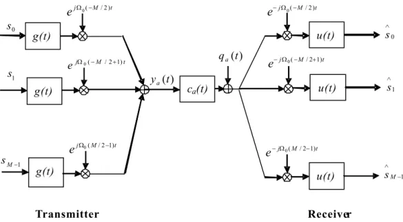
(18) e jW s0. 0. ( - M / 2 )t. e- j W. ( - M / 2 )t Ù. u(t). g(t) e jW 0 ( - M. s1. q a (t ). / 2 + 1) t. y a (t ). e jW. 0. e- j W. 0 ( -M. s0. / 2+ 1) t Ù. u(t). ca(t). g(t). s M -1. 0. ( M / 2 -1) t. e - jW. 0( M. s1. / 2- 1) t Ù. g(t). u(t). Transmitter. s M -1. Receiver. Figure 2.1: The analog framework baseband model of OFDM system.. pulse shaping filter g(t) is usually a rectangular pulse of length T0 = 2π/Ω0 The pulse shaping filter g(t) is given,. g(t) =. (. √1 , Ts. , 0 6 t 6 Tall. 0. , otherwise. (2.1). Where Ts is the data interval, Ts = 2πM/Ω0 . Tall is the duration of an OFDM symbol and it contains Ts and guard interval (GI). Assuming the number of subcarriers, M, is even and the output of the transmitter is given by,. −1 k= M 2. ya (t) =. X. sk g(t)ejkΩ0 t. (2.2). k=− M 2. Assume the length of the impulse response of the channel is short than the length of the guard interval Tg , and it is static within a OFDM symbol interval. Then passing the continuous-time signal through the physical channel to generate r(t). The received signal r(t) is, 7.

(19) r(t) = ca (t) ∗ ya (t) + g(t) Z −∞ = ca (τ )ya (t − τ )dτ + q(t) ∞ Z Tg = ca (τ )ya (t − τ )dτ + q(t).. (2.3). 0. Where q(t) is white Gaussian noise with zeros mean and variance σn2 . At the receiver site, the filter u(t) is the match filter to the part [T g , Ta ll] of g(t). u(t) is given as,. u(t) =. (. g > (Tall − Tg ), , 0 6 t 6 Tall − Tg 0. , otherwise. (2.4). Since the length of the impulse response of the channel is shorter than the guard interval (GI) and the length of the receiving filter u(t) is Ts , the received signal of this block will not be contaminated by the pervious block. In other word, the system is interblock interference free (IBI-free). Then the output of the receiver filter of the kth subchannel is expression as,. sbk = r(t)e−jkΩ0 (t−Tg ) ∗ u(t)|t=Tall Z ∞ = r(τ )ejkΩ0 (t−T g) u(Tall − τ )dτ.. (2.5). −∞. The whole section introduces the structure of analog framework representation model of the OFDM system. These expressions that denote the outputs of each component are also shown above.. 2.2. Digital Framework OFDM System Model. Because the transmitter and the receiver are easily implemented by an inverse discrete Fourier transform (IDFT) and a discrete time Fourier transform (DFT) respectively. Therefore, in practice, we use the digital framework representation OFDM system 8.

(20) model and the OFDM transceivers are implemented digitally. The transmitter performs M -point IDFT, and M -point DFT for receiver. M means the numbers of subchannels there. The P/S (parallel to series) converts parallel data samples into series ones. Every block contains M data samples. Following the P/S converter is cyclic prefix (CP) of length ν. The CP is added in front of data block, and CP is the last ν samples of the transmitted data block. In order to avoid interblock interference (IBI), the length of CP is chosen no smaller than the order of the channel. In order to transmit the data pass through physical channel, , we need D/C and C/D converters to work before transmitting data samples into the physical channel and CP removal operation respectively. Different from the transmitter, CP removal, S/P (series to parallel), and M -point DFT are performed in order at the receiver side. Finally, the DFT outputs are multiplexing a set of scalars, frequency domain equalizers (FEQs), to remove the gain resulted from channel. The block diagram of the digital framework representation OFDM system model is shown in Figure 2.2. n o is e M-pt ID F T. P/S. C y c lic pr e f ix. D /C. channel. Å. C /D. pr e f ix re m o v a l. S/P. M-pt D FT. FE Q. Figure 2.2: The digital framework baseband model of OFDM system.. 2.3. Analog Framework System Model Versus Digital Framework System Model. Many studies on OFDM systems are carried out from (2.2). That is the output of the transmitter of the analog framework OFDM system model. The pulse shaping filter g(t) is usually a rectangular pulse as mentioned in section 2.1. And we know that the analog framework model of the OFDM system is only useful for analysis, in practice, the OFDM system implemented in the discrete-time. We want 9.

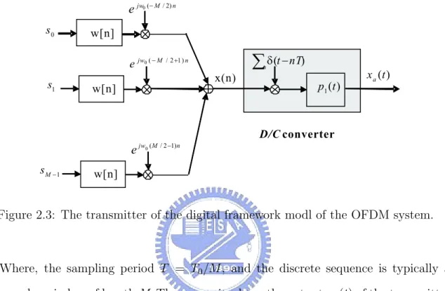
(21) to show the there is the considerable difference between the outputs of the transmitter of these two OFDM system models. For convenience of derivation, we redraw the Figure 2.2 as Figure 2.3 to focus on the transmitter of the digital framework representation OFDM system model. e jw0 (- M / 2) n s0. w[n] e jw0 ( - M. s1. å d (t - nT). / 2 +1 ) n. n. x(n). x a (t ). p1 (t ). w[n]. D/C converter. e sM -1. jw0 ( M / 2 -1) n. w[n]. Figure 2.3: The transmitter of the digital framework modl of the OFDM system.. Where, the sampling period T = T0 /M , and the discrete sequence is typically a rectangular window of length M. Then we write down the output xa (t) of the transmitter in Figure 2.3.. M 2. xa (t) =. Σ∞ n=−∞ x[n]p1 (t. − nT ), where, x[n] = w[n]. −1 X. 2π. sk ej( M )kn .. (2.6). k=− M 2. Our purpose is to show that given a discrete window w[n]and reconstruction filter , and there may not exist a corresponding pulse shaping filter. Therefore, it is impossible to analyze the outputs of the transmitter of the digital framework OFDM system model using the outputs of the transmitter of analog framework OFDM system model. Analyses of OFDM system directly using the digital framework OFDM system model are more useful than the analog schematic.. 10.

(22) We use the commonly used case of a rectangular window w[n] and an ideal lowpass reconstruction filter for derivation. The window of the OFDM transmitter is a rectangular window w[n],. w[n] =. (. 1, , 0 6 n 6 M − 1 0. , otherwise. (2.7). And the reconstruction filter of the transmitter is an ideal lowpass filter,. P1 (jΩ) =. (. 1, , | Ω |<. 0. π T. , otherwise. (2.8). Taking the expressions of w[n] and to rewrite xa (t) as. xa (t) = Σ. M −1 2 −M 2. xk. M −1 X n=0. 2π. ej( M )kn p1 (t − nT ).. (2.9). Comparing the expressions (2.2) and (2.9),and we conclude that xa (t) and ya (t) are equal for an arbitrary sequence sn if and only if there exists g(t)such that. g(t)e. jkΩ0 t. =. M −1 X n=0. 2π. ej( M )kn p1 (t − nT ), f ork = −. M M M ,− = 1, ..., − 1. 2 2 2. (2.10). PM −1 jΩ0 t When k = 0, we have g(t) = = n=0 p1 (t − nT ). When k = 1, we have g(t)e PM −1 j( 2π )n M p1 (t − nT ). Let f1 (t) = ejΩ0 t p1 (t), and using the definition Ω0 = M2πT , we n=0 e. can rewrite the equality expression as. M −1 g(t) = Σn=0 f1 (t − nT ).. (2.11). Then we can get the relationship between p1 (t) and f1 (t).. 2π. f1 (t) = e−j M T p1 (t). 11. (2.12).

(23) M −1 , and we can verify that Σn=0 p1 (t − nT ) 6=. PM −1 n=0. f1 (t − nT ). And the solution of g(t). obtained for k = 1 contradicts that for k = 0.. Therefore, we can conclude that there may not exist a pulse shaping filterg(t) for given w [n] and reconstruction filter . The outputs of the transmitter in these two kinds of OFDM system models are different. Because we implement the OFDM system digitally, the better way to analyze OFDM system is using the digital framework representation OFDM system model.. 12.

(24) Chapter 3 System Model Wireless local area networks (LANs) transmit data through orthogonal frequency division multiplexing (OFDM) systems. Because of the large number of subcarriers, OFDM system has high peak to average power ratio (PAPR). Therefore, the PAPR reduction is the important issue for OFDM system. We will introduce the PAPR concept in this chapter and the reason that makes OFDM system has high PAPR. When we implement OFDM system for communication, the continuous-time channel is a fading channel. We will introduce the fading channel that used for simulation in this thesis. The continuous-time channel and the infinite impulse response (IIR) transmitting and receiving pulses that makes the simulation hard to operate. In order to make simulation easier for operating, we will also transfer the part that includes transmitting pulse, continuous-time channel, and receiving pulse, to its equivalent discrete-time channel in this chapter. For the same reason, we introduce the discrete-time form of the continuoustime noise. The bit error rate (BER) performance is affected by the transmitting and receiving pulses design, so the BER is introduced there, too.. 3.1. Peak to Average Power Ratio (PAPR). Before the signal transmitted into the physical channel, it needs to pass through a power amplifier. Because the orthogonal frequency division modulation (OFDM) is one 13.

(25) kind of multitone modulation system, the power of each subcarrier changes at different time. The phenomenon results in the power amplifier operated in large linear region. In order to operate the power amplifier in high efficient region, the transmitted signals are clipped to make errors. Therefore, In practice, the transmitted system is peak power restrict. We expect the system operated in the perfect linear region that often means the average power level below the maximum power available. If the gap between the peak and average power values of transmitted signals is large, the power amplifier works on the low efficiency zone. In order to operate the power amplifier with higher efficiency, we expect to decrease the gap between the peak and average power values of the transmitted signals. The PAPR of the discrete-time signal is defined as,. P AP R =. maxn | x(n) |2 . E[| x(n) |2 ]. (3.1). The x is obtained by unblocking the IDFT output vector and adding a cyclic prefix. Therefore, the transmitter output has the same peak power and average power as the IDFT outputs xn and we can consider the ratio. maxn | x(n) |2 E[| x(n) |2 ]. (3.2). Instead of the PAPR of x. The output vector of the IDFT matrix xn = W + s, and its autocorrelation matrix Rx is given by. Rx = E[xx† ] = W† Rs W = εs IM. (3.3). Because the input vector s is uncorrelated, xn is also uncorrelated and their variances are the same, equal to εs . That can be express as. 14.

(26) E[max | x(n) |2 ] = εs , n = 0, 1, ..., M. n. The output of the IDFT matrix xn =. | xn |=|. M −1 X k=0. PM −1 k=0. 2πkn √1 sk ej M , M. and. M −1 √ 1 X 1 j 2πkn M |≤ √ | sk |≤ M max | sk | . sk √ e k M M k=0. So we have maxn | xn |=. (3.4). (3.5). √ M maxk sk .. The maximum value can be attained. For example, when all input symbols have √ the same value, we can obtain the maximum value M maxk | sk |. And the value of inputs are set as | sn |= maxk | sk |. Then turning to compute the PAPR value by the expression above,. P AP R = M. maxk | s(k) |2 . E[| s(k) |2 ]. (3.6). The PAPR of OFDM system is M times the PAPR of the input modulation symbol. For some applications of OFDM system, the IDFT matrix size M is large, for instance, M can be as larger as 2048 for fixed broadband wireless access systems. Because M is usually large for the OFDM systems, the PAPR value is large. That is why the PAPR reduction is the popular issue for the OFDM systems. There are many methods proposed to reduce PAPR, e.g. partial transmitted sequence (PTS) method, selective mapping (SLM), Clipping, and so on. In fact, when we discuss the PAPR problem, we use the more precise PAPR measurement in practice. That is done with continuous-time transmitted signal, that is. P AP Rt =. maxt | xa (t) |2 . E[| xa (t) |2 ] 15. (3.7).

(27) Where the subscript t denotes the PAPR value is computed from continuous-time transmitted signals. But we can not get the through the continuous-time transmitted signals directly. We can only predict the P AP Rt by P AP RL . The P AP RL value is come from the discretetime signal x. The subscript L means the oversampling rate. When L is 2, the sampling period is one half of the original sampling period. Then the sampling rate is twice. By the way, oversampling factor L is 1 means there is no oversampling, and the sampling rate is the same as the Niquist rate. Define P AP RL the as. P AP RL =. maxn | xL (n) |2 . E[| xL (n) |2 ]. (3.8). xL is produced by sampling the continuous-time xa (t) transmitted signal .The sampling period is T. The expression of xL is given as. T xL (n) = xa (n ) L ∞ X T = x(k)p1 (n − kT ). L k=−∞. (3.9). The process from discrete-time signal to is shown in Figure 3.1. t=T/L. x a (t ) x(n ). x L (n). D /C Oversampling(L). Figure 3.1: The Process of producing xL (n). The data stream x(n) is the form ±1±j. Therefore, from (3.8), we can view as linear combinations of sampled points of transmitting pulse p1 (t) with unit gain. Then the impulse response of transmitting pulse affects the PAPR performance. If the combination 16.

(28) of the sampled points of transmitting pulse has large peak to average power ratio, the PAPR performance is worse. Pay attention that the part of producing xL (n) by oversampling the continuous-time signal xa (t) is only for computing the PAPR value. The oversampling component is not really a part of our system model. As increasing the oversampling factor, the P AP RL value is more and more close to the P AP RL value. Then we use this method the get the approximate P AP RL value. The trade-off is the larger oversampling factor waste computation. We expect the use the least oversampling factor to use the lower computation to get the desired information. By definition, xa (t)is produced from the D/C converter reconstruction filter p1 (t), so the PAPR value depends on the reconstruction filter p1 (t) of the D/C converter at the transmitter, too. Therefore, choosing different reconstruction filter p 1 (t), result in some difference of the PAPR values. Generally speaking, the pulses at the transmitter and the receiver sides would be taken ideal lowpass filters for analyzing OFDM systems. Therefore, the affect coming from transmitting and receiving pulses is ignored as computing the PAPR value. The oversampling factor L is taken 4 for most PAPR analysis papers. But, from the definition of the , we know the choice of the D/C reconstruction filter affects the value. But general PAPR analysis paper set the reconstruction filter p1 (t) as ideal low-pass, and ignoring the effect comes from the transmitting pulse. Besides, we usually compute the PAPR value based on the analog OFDM system which introduced in chapter 2. But the practical implemented OFDM system is digital ODFM system. These two kinds of OFDM systems result in different continuous-time signal xa (t) that is mentioned in chapter 2. Owing to the distinct continuous-time signal xa (t), the P AP RL value is also different. There must be some error when we using the analog OFDM system to compute the P AP RL value. In order to get the more precise P AP RL value in the practical environment, we will use the digital OFDM system and. 17.

(29) some cases of realizable analog filter to simulate the transmitting and receiving pulses in the thesis. The complementary cumulative distribution function (CCDF) is the most used method for measuring the performance of PAPR. The CCDF of the PAPR denotes that the probability that the PAPR of a data stream exceeds a given threshold (P AP R0 ). The CCDF is defined as,. CCDF (P AP R0 ) = prob(P AP R > P AP R0 ).. (3.10). Under the same threshold P AP R0 , the smaller value of CCDF means the PAPR performance is better.. 3.2. Continuous-Time Fading Channel. Wireless systems are usually used operated inside the building, and it is known that the indoor radio channels are characterized by the presence of fading channel. Where, we investigate the performance of IEEE 802.11a wireless LANs operated on Rayleigh fading channels to model the indoor radio channels. The channel impulse is given,. ca (t) =. m X l=0. αl ejθl δ(t − lTs ).. (3.11). Where αl is the lth fading path gain, and it is a Rayleigh distributed random variable with a variance, α¯l2 . The means the lth faded path phase that is uniform distributed random variable over [0, 2π). m is the number of taps of the continuous time channel model and Ts is the sampling time. The channel dispersion is modeled by an exponential function and assumed the channel has unit gain,. ¯2 Σm l=0 αl = 1. 18. (3.12).

(30) We can set the variable m larger than the cyclic prefix (CP) length to simulate the environment without inter block interference (IBI), or smaller than CP length for the inter block interference free (IBI-free) environment. The CP can remove the effect of inert block interference (IBI) only when the length of CP is longer than the length of equivalent discrete-time channel. The number of taps of the continuous-time channel affects the length of equivalent discrete time channel. The larger the number of the taps of the continuous-time channel is, the longer the length of the equivalent discretetime channel is. In the thesis, m set to 2 to simulate the environment with inter block interference free (IBI-free).. 3.3. Equivalent Discrete-Time Channel. It is more convenient for us to work on a discrete-time system. Therefore, we want to find out the equivalent discrete-time channel of the OFDM system. Then we need to transfer the part from transmitting pulse to receiving pulse to its equivalent discretetime channel. The diagram from x to ris shown in Figure 3.2. The desired equivalent discrete-time channel is shown in Figure 3.3.. q a (t ). å d (t - nT) x(n). n. t = nT r(n). p1 (t ). p 2 (t ). c a (t ) ra (t ). x a (t ). w a (t ). C/D converter. D/C converter. Figure 3.2: The part from x(n) to r(n). Suppose the data samples x are spaced apart by T seconds and D/C converter produces a continuous-time signal xa (t) by passing x through a transmitting pulse p1 (t). That is 19.

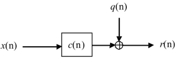
(31) q(n). x(n). c(n). r(n). Figure 3.3: The equivalent discrete-time channel. xa (t) = Σ∞ k=−∞ x(k)p1 (t − kT ).. (3.13). Then the received signals after the channel is. ra (t) = (xa ∗ ca )(t) + qa (t) = Σ∞ k=−∞ x(k)(p1 ∗ ca )(t − kT ) + qa (t).. (3.14). The wa (t) is obtained by passing ra (t) through the receiving pulse p2 (t),. wa (t) = (ra ∗ p2 )(t) = Σ∞ k=−∞ x(k)(p1 ∗ ca ∗ p2 )(t − kT ) + qa (t).. (3.15). Sampling every T seconds to get discrete-time output, r(n), Define the equivalent channel and noise as follows,. r(n) = w(nT ) = Σ∞ k=−∞ x(k)(p1 ∗ ca ∗ p2 )(nT − kT ) + (qa ∗ p2 )(nT ).. (3.16). Define the equivalent channel and noise as follows,. ce (t) = (p1 ∗ ca ∗ p2 )(t). 20. (3.17).

(32) and qe (t) = (qa ∗ p2 )(t).. (3.18). The received signal r(n) can be rewritten as. r(n) = Σ∞ k=−∞ x(k)c(n − k) + q(n).. (3.19). Discrete-time equivalent channel and noise are given by. c(n) = (p1 ∗ ca ∗ p2 )(t) |t=nT 0 .. (3.20). q(n) = (qa ∗ p2 )(t) |t=nT 0 .. (3.21). Where c(n) is the equivalent discrete-time channel, and ca (t) is the continuous-time channel, p1 (t)and p2 (t) representD/C converter and C/D converter analog filter respectively. c(n) is produced by sampling the output of continuous-time convolution of p 1 (t), ca (t), and p2 (t). In (3.11), q(n) is the equivalent discrete-time noise. Choosing different transmitting and receiving pulses, p1 (t) and p2 (t), will produce different discrete-time equivalent channels. And the length of the equivalent discretetime channel is inverse proportional to the sampling period T. Changing the sampling period to twice than the original one will reduce the length of c(n) to one half. When we already have the continuous-time channel, and the next step is to find out the equivalent discrete-time channel. The equivalent discrete-time channel model is shown in Figure 3.3, and its expression is also shown as (3.10) Owing to the infinite impulse response (IIR) filters, p1 (t) and p2 (t), the length of the result of the convolution is infinite, we need to truncate the result to be finite for our simulation. In order to do truncation, we sum the power of elements of the result 21.

(33) at first. We know almost 99 percentage power are concentrate on the former elements of the sampled points. Therefore, we just need to take the former elements to represent the behavior of OFDM system channel.. 3.4. Noise Generation. After the channel noise qa (t) passes through the receiving pulse p2 (t), it is no longer white noise. The block diagram is in Figure. 3.4. t = nT q a (t ). p 2 (t ). q (n) n a (t ). Figure 3.4: Channel noise of the digital framework OFDM system model. Because we can not directly produce continuous-time noise qa (t) for our simulation, we expect to design a filter f(n). Setting a series discrete-time white noise n w through the f(n), and we can obtain another discrete-time color noise q0 that has the same statistic characteristics as q. The system block diagram is shown in Figure 3.5.. n w (n ). f (n). q ' (n ). Figure 3.5: The equivalent discrete-time channel. First, the autocorrelation function of q, Rq (k), is the information we can easily compute in advance if we know the properties of the receiving pulse p2 (t). Then just go to computer the autocorrelation of q , that is,. Rq (k) = E[q(n)q† (n + k)]. On the other hand, the autocorrelation function of na (t) is shown as follows, 22. (3.22).

(34) Rna (τ ) = E[na (t)n†a (t + τ )].. (3.23). By Figure 3.5, the noise q is produced by sampling the noise na (t), and it can be expressed as. q(n) = na (nT ),. (3.24). where T is the sampling period. From the above expression, we expect the autocorrelation functions between qand na (t) must has some relationship. Therefore, we can take the above expression into these two autocorrelation functions, that is,. Rq (k) = E[q(n)q† (n + k)] = E[na (nT )n∗a ((n + k)T )] = Rna (kT ).. (3.25). The autocorrelation function Rq (k) could be viewed as the autocorrelation function of na (t) which sampled by every T seconds.. Rq (k) = Rna (kT ).. (3.26). Look at the first part of the block diagram of channel noise. The continuous time color noise na (t) is given by passing continuous-time white noise qa (t) through the receiver pulse p2 (t). On this option, the also shown as,. Rna (k) = N0 p2 (τ ) ∗ p∗2 (τ ).. (3.27). Where N0 is the autocorrelation of white noise qa (t). Then we can obtain the power spectrum of na (t) by taking the Fourier transform of the above expression, 23.

(35) Sna (jΩ) = N0 | P2 (jΩ) |2 .. (3.28). Because Rq (k) = Rna (kT ), we can sample the Sna (jΩ) by every T seconds to obtain the power spectrum of q , that is. ∞ w 2πk 1 X Sna (j( − )) Sq (e ) = T k=−∞ T T jw. ∞ 1 X w 2πk 2 = N0 | P2 (j( − )) | . T k=−∞ T T. (3.29). Finally, we come to design the filter f(n). Then we can input discrete-time white noise q0 into f(n) to obtain discrete-time color noise which has the same power spectrum as that of q ,. Sq (ejw ) =. ∞ w 2πk 2 1 X N0 | P2 (j( − )) | T k=−∞ T T. = N0 | F (ejw ) |2 .. (3.30). When we get the F (ejw ), then taking inverse Fourier transform to obtain the desired filter f(n), this is. 2π. f (n) = IDF T (F (ej M k)).. (3.31). Take this processes, we can easily generate the discrete-time colored noise q0 by putting discrete-time white noise nw through the filter f(n). The discrete-time colored noise q0 has the same statistic properties with the discrete-time noise q.. 3.5. Bit Error Rate. In order to analyze the effect of the channel noise, we only draw the noise path at the receiver side in Figure. 3.6. The elements of the continuous-time white noise q a (t) 24.

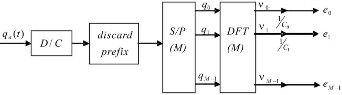
(36) series are uncorrelated with variance N0 . After qa (t) passed through the D/C converter, the discard prefix, and the S/P, the elements of the blocked color noise q are correlated. Of course, the variance of q is not the same as qa (t). The autocorrelation matrix of q is denoted as Rq .. q0. n0. e0. 1. q a (t ). D/ C. discard. S/P. prefix. (M). q1. DFT. n1. e1. 1. (M) q M -1. C0 C1. n M -1. e M -1. Figure 3.6: The equivalent discrete-time channel.. The noise vector ν at the output of the DFT matrix is produced by q. Then the noise vector ν has autocorrelation matrix. Rν = E[νν † ] = E[Wqq† W† ] = WRq W† . The kth subchannel error ek =. νk . Ck. (3.32). Owing to the effect of FEQs, there are different. variances for each subchannel error. The variance of ek is. σe2k. σν2k = | C k |2. (3.33). where, σν2k is the variance of νk . The SNR of the kth subchannel β(k) =. εs 2 σek. which is dependent on the channel. response Ck . The denotes signal power over noise power ratio. The noise is the discretetime noise q in the equivalent discrete-time channel shown in Figure.3.3. The SNR defined in the thesis is given, 25.

(37) SN R =. εs , σq2. (3.34). where εs is the signal power and σq2 is the noise variance of noise q. For QPSK modulation with power , and the symbol has the form ±. p εs 2. ±. p εs 2. . In. this case the BER can be computed by Q-function. The BER of the kth subchannel is. BER(k) = Q(. p β(k)).. The average BER of the OFDM system is given by BERav =. (3.35) 1 M. PM −1 k=0. BER(k).. From (3.30) and (3.32), we can know that the average BER of OFDM system is affected by the channel response Ck . When the channel response Ck is larger, the average BER is smaller. In other words, the system has better BER performance.. 26.

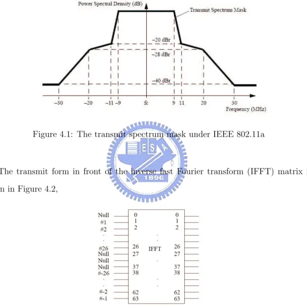
(38) Chapter 4 Numerical Simulation In this chapter, we will give four cases of elliptic analog filter design that based on the IEEE 802.11a wireless LANs. We observe these examples to show how the filter design affects the peak to average power ratio (PAPR), oversampling factor L, and bit error rate (BER) performance. In case 1, we use different stopband edge to produce distinct the useful band bandwidths. In case 2, we adjust the passband and stopband edge to have different useful band bandwidths, and their have the same transition band bandwidths that center at sampling frequency (fs). In case 3, we use different passband edge to produce distinct useful band bandwidths. In case 4, we change passsband and stopband edge to get the same transition band bandwidth, and their useful band bandwidths are the same. The detail parameters of designing elliptic analog filter are introduced in each case. In these simulations, we use two kinds of the continuous-time channels: Rayleigh fading channel and additive white Gaussian noise (AWGN) channel. The data stream use quadrature phase-shift keying (QPSK) modulation, and the mapped signals have the form ±1 ± j. All these cases are simulated under inter block interference (IBI-free) environment. In other words, the length of the equivalent discrete-time channel is longer than the cyclic prefix (CP) in all cases. The IEEE 802.11a wireless LANs use the inverse fast Fourier transform (IFFT) to. 27.

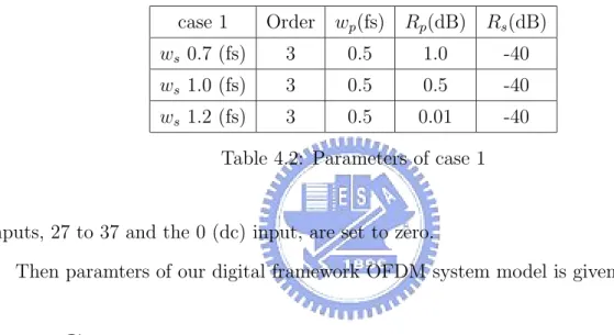
(39) substitute for the inverse discrete Fourier transform (IDFT) at the transmitter site. The IEEE 802.11a standard restricts the power of the transmitted signal and the transmit form of transmitted signal before passing trough the IFFT matrix. The restriction about the power of transmitted signal is given in Figure 4.1,. Figure 4.1: The transmit spectrum mask under IEEE 802.11a. The transmit form in front of the inverse fast Fourier transform (IFFT) matrix is given in Figure 4.2,. Figure 4.2: The form of inputs for IFFT matrix. The coefficients from 1 to 26 are mapped to the same numbered IFFT inputs, while the coefficients from -26 to -1 are copied into IFFT inputs 38 to 63. The rest of the 28.

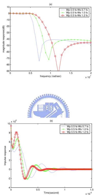
(40) Subcarrier (N). 52. IDFT size (M). 64. CP length (ν). 16. Sampling time (T). 10−7 second. Modulation. QPSK. Symbol blocks. 106. Numbers of taps of ca (t). 2. Numbers of random channel ca (t). 105. Table 4.1: Parameters of digital framework OFDM system case 1. Order wp (fs) Rp (dB) Rs (dB). ws 0.7 (fs). 3. 0.5. 1.0. -40. ws 1.0 (fs). 3. 0.5. 0.5. -40. ws 1.2 (fs). 3. 0.5. 0.01. -40. Table 4.2: Parameters of case 1. inputs, 27 to 37 and the 0 (dc) input, are set to zero. Then paramters of our digital framework OFDM system model is given,. 4.1. Case 1. The analog filters taken for simulation are elliptic analog filters. We want to see if the useful band bandwidth affects the PAPR performance and the BER performance. Fix the passband edge, passband ripple, and stopband attenuation. Then we change stopband edge to produce distinct useful band bandwidths. The transmitting and receiving pulses, p1 (t) and p2 (t), are chosen the same when we simulate the BER performance. In other words, we have three kinds of analog filters, and we have three BER performance curves in this case. The parameters of filter design are given in table 4.2. The magnitude response of each filter in frequency domain and the impulse response of each filter in time domain are shown in Figure 4.3(a) and Figure 4.3(b). 29.

(41) (a). 10. Wp 0.5 fs-Ws 0.7 fs Wp 0.5 fs-Ws 1.0 fs Wp 0.5 fs-Ws 1.2 fs. 0. magnitude response(dB). -10 -20 -30 -40 -50 -60 -70 -80 -90. 0. 0.5. 1 frequency (rad/sec). 6. 10. 1.5. 2 7. x 10. (b). x 10. Wp 0.5 fs-Ws 0.7 fs Wp 0.5 fs-Ws 1.0 fs Wp 0.5 fs-Ws 1.2 fs. 8. Impulse response. 6 4 2 0 -2 -4. 0. 0.5. Time(second). 1. 1.5 -6. x 10. Figure 4.3: (a)The magnitude responses (b)The impulse responses of elliptic analog filters with distinct stopband edges.. 30.

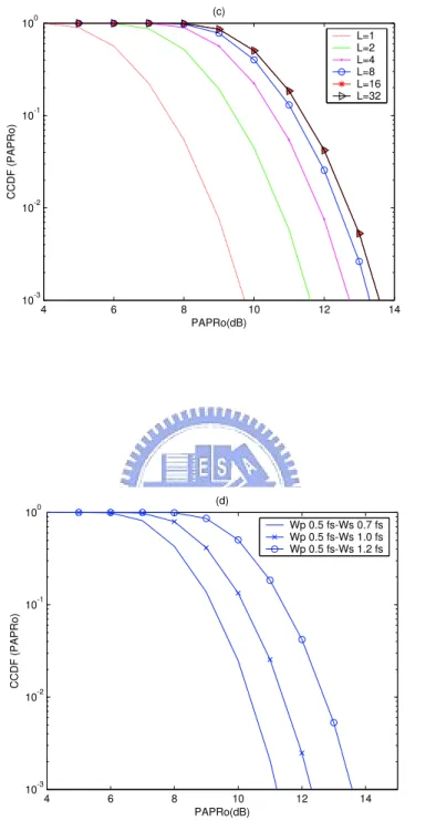
(42) 4.1.1. Peak to Average Power Ratio. There we will take (3.8) to compute the peak to average power ratio (PAPR) value, and the PAPR performance curves are shown in Figure 4.4. We use oversampling factors (L) = 1, 2, 4, 8, 16, and 32 respectively to simulate the PAPR performance for each filter. Then we also focus on which factor is the least oversampling factor that we need to use for computing the PAPR value.. 4.1.2. Bit Error Rate. The bit error rate (BER) performance comes from the average of 105 random channels. In this section, we show the average BER performance of Rayleigh fading channel and additive white Gaussian noise channel. At first, we deal with the Rayleigh fading channel. We take one of the 105 random continuous-time fading channels for example to show impulse response, magnitude response, and the BER performance of its equivalent discrete-time channel c1 (n) in Figure 4.5. (θ1 : 5.6165, θ2 : 1.2512; α1 : 1.3951, α2 : 0.6319). When the continuous-time channel is AWGN channel, its equivalent discrete-time channel is c2 (n). The impulse response, magnitude response, and the BER performance of c2 (n) is shown in Figure 4.6. From these simulation results, we can know that: 1. Oversampling factor: We need to take oversampling factor L = 16 to get the PAPR closer to the continuous-time PAPR. L = 4 is not enough for used. 2. PAPR performance: When the stopband edge of filer is large (ws = 1.2f s), it has large useful band bandwidth. Its PAPR performance is worse. 3. BER performance: When the useful band bandwidth is large, the filter has better BER performance.. 31.

(43) (a). 0. 10. L=1 L=2 L=4 L=8 L=16 L=32. -1. CCDF (PAPRo). 10. -2. 10. -3. 10. 4. 5. 6. 7. 8 PAPRo(dB). 9. 10. 11. 12. (b). 0. 10. L=1 L=2 L=4 L=8 L=16 L=32. -1. CCDF (PAPRo). 10. -2. 10. -3. 10. 4. 5. 6. 7. 8 9 PAPRo(dB). 32. 10. 11. 12. 13.

(44) (c). 0. 10. L=1 L=2 L=4 L=8 L=16 L=32. -1. CCDF (PAPRo). 10. -2. 10. -3. 10. 4. 6. 8. PAPRo(dB). 10. 12. 14. (d). 0. 10. Wp 0.5 fs-Ws 0.7 fs Wp 0.5 fs-Ws 1.0 fs Wp 0.5 fs-Ws 1.2 fs. -1. CCDF (PAPRo). 10. -2. 10. -3. 10. 4. 6. 8. 10 PAPRo(dB). 12. 14. Figure 4.4: The PAPR curves of elliptic analog filters with distinct stopband edges w s . (a) ws is 0.7 fs. (b)ws is 1.0 fs. (c) ws is 1.2 fs. (d) The PAPR curves of these three filters and the oversampling factor is 32.. 33.

(45) (a). 0.1. Wp 0.5 fs-Ws 0.7 fs Wp 0.5 fs-Ws 1.0 fs Wp 0.5 fs-Ws 1.2 fs. 0.08 0.06. Impulse response. 0.04 0.02 0 -0.02 -0.04 -0.06 -0.08 -0.1. 0. 0.5. Time (second). 1. 1.5 -6. x 10. (b). 20. magnitude response(dB). 0. -20. -40. -60. -80. -100. Wp 0.5 fs-Ws 0.7 fs Wp 0.5 fs-Ws 1.0 fs Wp 0.5 fs-Wp 1.2 fs 0. 0.2. 0.4 0.6 normalized frequency. 34. 0.8. 1.

(46) (c). 0. 10. Wp 0.5 fs-Ws 0.7 fs Wp 0.5 fs-Ws 1.0 fs Wp 0.5 fs-Ws 1.2 fs. -1. BER. 10. -2. 10. -3. 10. -4. 10. 0. 5. 10. 15 20 SNR(dB). 25. 30. 35. Figure 4.5: (a) The impulse response (b) The magnitude response (c) BER performance of c1 (n). (a). 0.1. Wp 0.5 fs-Ws 0.7 fs Wp 0.5 fs-Ws 1.0 fs Wp 0.5 fs-Ws 1.2 fs. 0.08 0.06. Impulse response. 0.04 0.02 0 -0.02 -0.04 -0.06 -0.08 -0.1. 0. 0.5. Time (second). 35. 1. 1.5 -6. x 10.

(47) (b). 100. magnitude response(dB). 50. 0. -50. -100. -150. -200. Wp 0.5 fs-Ws 0.7 fs Wp 0.5 fs-Ws 1.0 fs Wp 0.5 fs-Wp 1.2 fs 0. 0.2. 0.4 0.6 normalized frequency. 0.8. 1. (c). 0. 10. Wp 0.5 fs-Ws 0.7 fs Wp 0.5 fs-Ws 1.0 fs Wp 0.5 fs-Ws 1.2 fs. -1. BER. 10. -2. 10. -3. 10. -4. 10. 0. 2. 4. 6. 8 SNR(dB). 10. 12. 14. 16. Figure 4.6: (a) The impulse response (b) The magnitude response (c) BER performance of c2 (n). 36.

(48) case 2. Order ws (fs) Rp (dB) Rs (dB). wp 0.2(fs). 2. 1.8. 1.0. -40. wp 0.5(fs). 2. 1.5. 1.0. -40. wp 0.8(fs). 3. 1.2. 1.0. -40. Table 4.3: Parameters of case 2. 4.2. Case 2. The analog filters taken for simulation are elliptic analog filters. We want to see if the useful band bandwidth affects the PAPR performance and the BER performance. Fix the passband ripple and stop attenuation, then using different passband edge and stopband edge to produce distinct useful band bandwidths. The transition bands center at 1.0 sampling frequency (fs). The transmitting and receiving pulses, p1 (t) and p2 (t), are chosen the same when we simulate the BER performance. In other words, we have three kinds of analog filters, and we have three BER performance curves in this case. The parameters of filter design are given in table 4.3. The magnitude response of each filter in frequency domain and the impulse response of each filter in time domain are shown in Figure 4.7.. 4.2.1. Peak to Average Power Ratio. There we will take (3.8) to compute the peak to average power ratio (PAPR) value, and the PAPR performance curves are shown in Figure 4.8. We use oversampling factors (L) = 1, 2, 4, 8, 16, and 32 respectively to simulate the PAPR performance for each filter. Then we also focus on which factor is the least oversampling factor that we need to use for computing the PAPR value.. 37.

(49) (a) Wp 0.2 fs-Ws 1.8 fs Wp 0.5 fs-Ws 1.5 fs Wp 0.8 fs-Ws 1.2 fs. 0. magnitude response(dB). -20. -40. -60. -80. -100 0. 0.5. 1 frequency (rad/sec). 6. 12. 1.5. 2 7. x 10. (b). x 10. Wp 0.2 fs-Ws 1.8 fs Wp 0.5 fs-Ws 1.5 fs Wp 0.8 fs-Ws 1.2 fs. 10. Impulse response. 8 6 4 2 0 -2 -4 -6. 0. 0.5. Time(second). 1. 1.5 -6. x 10. Figure 4.7: (a)The magnitude responses (b)The impulse responses of elliptic analog filters with distinct transition band bandwidths which center at 1.0 fs.. 38.

(50) (a). 0. 10. L=1 L=2 L=4 L=8 L=16 L=32. -1. CCDF (PAPRo). 10. -2. 10. -3. 10. 4.2.2. 4. 5. 6. 7. 8 PAPRo(dB). 9. 10. 11. 12. Bit Error Rate. The bit error rate (BER) performance comes from the average of 105 random channels. In this section, we show the average BER performance of Rayleigh fading channel and additive white Gaussian noise channel. At first, we deal with the Rayleigh fading channel. We take one of the 105 random continuous-time fading channels for example to show impulse response, magnitude response, and the BER performance of its equivalent discrete-time channel c3 (n) in Figure 4.9. (θ1 : 0.36374, θ2 : 2.21710; α1 : 1.5683, α2 : 0.8305). When the continuous-time channel is AWGN channel, its equivalent discrete-time channel is c4 (n). The impulse response, magnitude response, and the BER performance of c4 (n) is shown in Figure 4.10. From these simulation results, we can know that: 1. Oversampling factor: We need to take oversampling factor L = 16 to get the PAPR closer to the continuous-time PAPR. L = 4 is not enough for used. 2. PAPR performance: When the filter has large useful band bandwidth (wp = 0.8f s, ws = 1.2f s), its PAPR performance is better. The one has smaller use39.

(51) (c). 0. 10. L=1 L=2 L=4 L=8 L=16 L=32. -1. CCDF (PAPRo). 10. -2. 10. -3. 10. 4. 6. 8. PAPRo(dB). 10. 12. 14. (c). 0. 10. L=1 L=2 L=4 L=8 L=16 L=32. -1. CCDF (PAPRo). 10. -2. 10. -3. 10. 4. 6. 8. PAPRo(dB). 40. 10. 12. 14.

(52) (d). 0. 10. Wp 0.2 fs-Ws 1.8 fs Wp 0.5 fs-Ws 1.5 fs Wp 0.8 fs-Ws 1.2 fs. -1. CCDF (PAPRo). 10. -2. 10. -3. 10. 4. 6. 8. 10 PAPRo(dB). 12. 14. Figure 4.8: The PAPR curves of elliptic analog filters with distinct transition band bandwidths. (a) wp is 0.2 fs and ws is 0.8 fs. (b)wp is 0.5 fs and ws is 1.5 fs. (c) wp is 0.8 fs and ws is 1.2 fs. (d) The PAPR curves of these three filters and the oversampling factor is 32.. (a). 0.1. Wp 0.2 fs-Ws 1.8 fs Wp 0.5 fs-Ws 1.5 fs Wp 0.8 fs-Ws 1.2 fs. 0.08 0.06. Impulse response. 0.04 0.02 0 -0.02 -0.04 -0.06 -0.08 -0.1. 0. 0.5. Time (second). 41. 1. 1.5 -6. x 10.

(53) (b). 20 0. magnitude response(dB). -20 -40 -60 -80 Wp 0.2 fs-Ws 1.8 fs Wp 0.5 fs-Ws 1.5 fs Wp 0.8 fs-Ws 1.2 fs. -100 -120. 0. 0.2. 0.4 0.6 normalized frequency. 0.8. 1. (c). 0. 10. Wp 0.2 fs-Ws 1.8 fs Wp 0.5 fs-Ws 1.5 fs Wp 0.8 fs-Ws 1.2 fs. -1. BER. 10. -2. 10. -3. 10. -4. 10. 0. 5. 10. 15 20 SNR(dB). 25. 30. 35. Figure 4.9: (a) The impulse response (b) The magnitude response (c) BER performance of c3 (n). 42.

(54) (a). 0.1. Wp 0.5 fs-Ws 0.7 fs Wp 0.5 fs-Ws 1.0 fs Wp 0.5 fs-Ws 1.3 fs. 0.08 0.06. Impulse response. 0.04 0.02 0 -0.02 -0.04 -0.06 -0.08 -0.1. 0. 0.5. Time (second). 1. 1.5 -6. x 10. (b). 40. magnitude response(dB). 20. 0. -20. -40. -60. -80. Wp 0.5 fs-Ws 0.7 fs Wp 0.5 fs-Ws 1.0 fs Wp 0.5 fs-Wp 1.3 fs 0. 0.2. 0.4 0.6 normalized frequency. 43. 0.8. 1.

(55) (c). 0. 10. Wp 0.2 fs-Ws 1.8 fs Wp 0.5 fs-Ws 1.5 fs Wp 0.8 fs-Ws 1.2 fs. -1. BER. 10. -2. 10. -3. 10. -4. 10. 0. 5. 10. SNR(dB). 15. 20. 25. Figure 4.10: (a) The impulse response (b) The magnitude response (c) BER performance of c4 (n). ful band bandwidth, and its PAPR performance is better. 3. BER performance: When the useful band bandwidth is large, the filter has better BER performance.. 4.3. Case 3. The analog filters taken for simulation are elliptic analog filters. We want to see if the useful band bandwidth affects the PAPR performance and the BER performance. Fix the stopband edge, passband ripple, and stopband attenuation. Then change passband edge to produce distinct useful band bandwidths. The transmitting and receiving pulses, p1 (t) and p2 (t), are chosen the same when we simulate the BER performance. In other words, we have three kinds of analog filters, and we have three BER performance curves in this case. The parameters of filter design are given in table 4.4. The magnitude response of each filter in frequency domain and the impulse response of each filter in time domain are shown in Figure 4.11.. 44.

(56) case 3. Order ws (fs) Rp (dB) Rs (dB). wp 0.2 (fs). 2. 1.5. 1.0. -40. wp 0.5 (fs). 3. 1.5. 1.0. -40. wp 0.8 (fs). 4. 1.5. 0.1. -40. Table 4.4: Parameters of case 3. (a). 10. Wp 0.2 fs-Ws 1.5 fs Wp 0.5 fs-Ws 1.5 fs Wp 0.8 fs-Ws 1.5 fs. 0. magnitude response(dB). -10 -20 -30 -40 -50 -60 -70 -80 -90 -100. 0. 0.5. 1 frequency (rad/sec). 6. 10. 1.5. 2 7. x 10. (b). x 10. Wp 0.2 fs-Ws 1.5 fs Wp 0.5 fs-Ws 1.5 fs Wp 0.8 fs-Ws 1.5 fs. 8. Impulse response. 6 4 2 0 -2 -4. 0. 0.5. Time(second). 1. 1.5 -6. x 10. Figure 4.11: (a)The magnitude responses (b)The impulse responses of elliptic analog filters with distinct passband edges.. 45.

(57) 4.3.1. Peak to Average Power Ratio. There we will take (3.8) to compute the peak to average power ratio (PAPR) value, and the PAPR performance curves are shown in Figure 4.12. We use oversampling factors (L) = 1, 2, 4, 8, 16, and 32 respectively to simulate the PAPR performance for each filter. Then we also focus on which factor is the least oversampling factor that we need to use for computing the PAPR value. (a). 0. 10. L=1 L=2 L=4 L=8 L=16 L=32. -1. CCDF (PAPRo). 10. -2. 10. -3. 10. 4. 5. 6. 7 PAPRo(dB). 8. 9. 10. (b). 0. 10. L=1 L=2 L=4 L=8 L=16 L=32. -1. CCDF (PAPRo). 10. -2. 10. -3. 10. 4. 5. 6. 7 8 PAPRo(dB). 46. 9. 10. 11.

(58) (c). 0. 10. L=1 L=2 L=4 L=8 L=16 L=32. -1. CCDF (PAPRo). 10. -2. 10. -3. 10. 4.3.2. 4. 5. 6. 7 8 PAPRo(dB). 9. 10. 11. Bit Error Rate. The bit error rate (BER) performance comes from the average of 105 random channels. In this section, we show the average BER performance of Rayleigh fading channel and additive white Gaussian noise channel. At first, we deal with the Rayleigh fading channel. We take one of the 105 random continuous-time fading channels for example to show impulse response, magnitude response, and the BER performance of its equivalent discrete-time channel c5 (n) in Figure 4.13. (θ1 : 4.994, θ2 : 6.012; α1 : 0.38437, α2 : 0.6352). When the continuous-time channel is AWGN channel, its equivalent discrete-time channel is c6 (n). The impulse response, magnitude response, and the BER performance of c6 (n) is shown in Figure 4.14. From these simulation results, we can know that: 1. Oversampling factor: We need to take oversampling factor L = 4 to get the PAPR closer to the continuous-time PAPR. 2. PAPR performance: When the passband edge of filer is large (wp = 0.8f s), it has large useful band bandwidth. Its PAPR performance is worse.. 47.

(59) (d). 0. 10. Wp 0.2 fs-Ws 1.5 fs Wp 0.5 fs-Ws 1.5 fs Wp 0.8 fs-Ws 1.5 fs. -1. CCDF (PAPRo). 10. -2. 10. -3. 10. 4. 5. 6. 7 8 PAPRo(dB). 9. 10. 11. Figure 4.12: The PAPR curves of elliptic analog filters with distinct passband edges w p . (a) wp is 0.2 fs. (b)wp is 0.5 fs. (c) wp is 0.8 fs. (d) The PAPR curves of these three filters and the oversampling factor is 32.. (a). 0.1. Wp 0.2 fs-Ws 1.5 fs Wp 0.5 fs-Ws 1.5 fs Wp 0.8 fs-Ws 1.5 fs. 0.08 0.06. Impulse response. 0.04 0.02 0 -0.02 -0.04 -0.06 -0.08 -0.1. 0. 0.5. Time (second). 48. 1. 1.5 -6. x 10.

(60) (b). 20 0. magnitude magnitude(dB). -20 -40 -60 -80 Wp 0.2 fs-Ws 1.5 fs Wp 0.5 fs-Ws 1.5 fs Wp 0.8 fs-Ws 1.5 fs. -100 -120. 0. 0.2. 0.4 0.6 normalized frequency. 0.8. 1. (c). 0. 10. Wp 0.2 fs-Ws 1.5 fs Wp 0.5 fs-Ws 1.5 fs Wp 0.8 fs-Ws 1.5 fs. -1. BER. 10. -2. 10. -3. 10. -4. 10. 0. 5. 10. 15 20 SNR(dB). 25. 30. 35. Figure 4.13: (a) The impulse response (b) The magnitude response (c) BER performance of c5 (n). 49.

(61) (a). 0.1. Wp 0.5 fs-Ws 0.7 fs Wp 0.5 fs-Ws 1.0 fs Wp 0.5 fs-Ws 1.3 fs. 0.08 0.06. Impulse response. 0.04 0.02 0 -0.02 -0.04 -0.06 -0.08 -0.1. 0. 0.5. Time (second). 1. 1.5 -6. x 10. (b). 50 0. magnitude response(dB). -50 -100 -150 -200 -250 -300 Wp 0.5 fs-Ws 0.7 fs Wp 0.5 fs-Ws 1.0 fs Wp 0.5 fs-Wp 1.3 fs. -350 -400. 0. 0.2. 0.4 0.6 normalized frequency. 50. 0.8. 1.

(62) (c). 0. 10. Wp 0.2 fs-Ws 1.5 fs Wp 0.5 fs-Ws 1.5 fs Wp 0.8 fs-Ws 1.5 fs. -1. BER. 10. -2. 10. -3. 10. -4. 10. 0. 5. 10. 15 SNR(dB). 20. 25. 30. Figure 4.14: (a) The impulse response (b) The magnitude response (c) BER performance of c6 (n). 3. BER performance: When the useful band bandwidth is large, the filter has better BER performance.. 4.4. Case 4. The analog filters taken for simulation are elliptic analog filters. We want to see if the useful band bandwidth affects the PAPR performance and the BER performance. Fix the transition band bandwidth, passband ripple, and stopband attenuation. Then change passband edge and stopband edge to produce distinct useful band bandwidths. The transmitting and receiving pulses, p1 (t) and p2 (t), are chosen the same when we simulate the BER performance. In other words, we have three kinds of analog filters, and we have three BER performance curves in this case. The parameters of filter design are given in table 4.5. The magnitude response of each filter in frequency domain and the impulse response of each filter in time domain are shown in Figure 4.15.. 51.

(63) case 4. Order ws (fs) Rp (dB) Rs (dB). wp 0.2 (fs). 4. 0.9. 0.01. -40. wp 0.5 (fs). 4. 1.2. 0.01. -40. wp 0.8 (fs). 4. 1.5. 0.01. -40. Table 4.5: Parameters of case 4. (a). 10. Wp 0.2 fs-Ws 0.9 fs Wp 0.5 fs-Ws 1.2 fs Wp 0.8 fs-Ws 1.5 fs. 0. magnitude response(dB). -10 -20 -30 -40 -50 -60 -70 -80 -90 -100. 0. 0.5. 1 frequency (rad/sec). 6. 10. 1.5. 2 7. x 10. (b). x 10. Wp 0.2 fs-Ws 0.9 fs Wp 0.5 fs-Ws 1.2 fs Wp 0.8 fs-Ws 1.5 fs. 8. Impulse response. 6 4 2 0 -2 -4. 0. 0.5. Time(second). 1. 1.5 -6. x 10. Figure 4.15: (a)The magnitude responses (b)The impulse responses of elliptic analog filters with the same transition band bandwidth.. 52.

(64) 4.4.1. Peak to Average Power Ratio. There we will take (3.8) to compute the peak to average power ratio (PAPR) value, and the PAPR performance curves are shown in Figure 4.12. We use oversampling factors (L) = 1, 2, 4, 8, 16, and 32 respectively to simulate the PAPR performance for each filter. Then we also focus on which factor is the least oversampling factor that we need to use for computing the PAPR value.. 4.4.2. Bit Error Rate. The bit error rate (BER) performance comes from the average of 105 random channels. In this section, we show the average BER performance of Rayleigh fading channel and additive white Gaussian noise channel. At first, we deal with the Rayleigh fading channel. We take one of the 105 random continuous-time fading channels for example to show impulse response, magnitude response, and the BER performance of its equivalent discrete-time channel c7 (n) in Figure 4.17. (θ1 : 2.3274, θ2 : 4.41541; α1 : 0.70429, α2 : 0.69466). When the continuous-time channel is AWGN channel, its equivalent discrete-time channel is c8 (n). The impulse response, magnitude response, and the BER performance of c8 (n) is shown in Figure 4.18. From these simulation results, we can know that: 1. Oversampling factor: We need to take oversampling factor L = 4 to get the PAPR closer to the continuous-time PAPR. 2. PAPR performance: When the filer has large useful band bandwidth (wp = 0.8f sandws = 1.5f s), its PAPR performance is worse. 3. BER performance: When the useful band bandwidth is large, the filter has better BER performance.. 53.

(65) (a). 0. 10. L=1 L=2 L=4 L=8 L=16 L=32. -1. CCDF (PAPRo). 10. -2. 10. -3. 10. 4. 5. 6. 7 PAPRo(dB). 8. 9. 10. (b). 0. 10. L=1 L=2 L=4 L=8 L=16 L=32. -1. CCDF (PAPRo). 10. -2. 10. -3. 10. 4. 5. 6. 7 8 PAPRo(dB). 54. 9. 10. 11.

(66) (c). 0. 10. L=1 L=2 L=4 L=8 L=16 L=32. -1. CCDF (PAPRo). 10. -2. 10. -3. 10. 4. 5. 6. 7 8 PAPRo(dB). 9. 10. 11. (d). 0. 10. Wp 0.2 fs-Ws 0.9 fs Wp 0.5 fs-Ws 1.2 fs Wp 0.8 fs-Ws 1.5 fs. -1. CCDF (PAPRo). 10. -2. 10. -3. 10. 4. 5. 6. 7 8 PAPRo(dB). 9. 10. 11. Figure 4.16: The PAPR curves of elliptic analog filters with the same transition band bandwidth and distinct useful band bandwidths. (a)wp is 0.2 fs and ws is 0.9 fs. (b)wp is 0.5 fs and ws is 1.2 fs. (c) wp is 0.8 fs and ws is 1.5 fs. (d) The PAPR curves of these three filters and the oversampling factor is 32.. 55.

(67) (a). 0.1. Wp 0.2 fs-Ws 0.9 fs Wp 0.5 fs-Ws 1.2 fs Wp 0.8 fs-Ws 1.5 fs. 0.08 0.06. Impulse response. 0.04 0.02 0 -0.02 -0.04 -0.06 -0.08 -0.1. 0. 0.5. Time (second). 1. 1.5 -6. x 10. (b). 20 0. magnitude magnitude(dB). -20 -40 -60 -80 -100 Wp 0.2 fs-Ws 0.9 fs Wp 0.5 fs-Ws 1.2 fs Wp 0.8 fs-Ws 1.5 fs. -120 -140. 0. 0.2. 0.4 0.6 normalized frequency. 56. 0.8. 1.

(68) (c). 0. 10. Wp 0.2 fs-Ws 0.9 fs Wp 0.5 fs-Ws 1.2 fs Wp 0.8 fs-Ws 1.5 fs. -1. BER. 10. -2. 10. -3. 10. -4. 10. 0. 5. 10. 15. 20 SNR(dB). 25. 30. 35. 40. Figure 4.17: (a) The impulse response (b) The magnitude response (c) BER performance of c7 (n). (a). 0.1. Wp 0.5 fs-Ws 0.7 fs Wp 0.5 fs-Ws 1.0 fs Wp 0.5 fs-Ws 1.3 fs. 0.08 0.06. Impulse response. 0.04 0.02 0 -0.02 -0.04 -0.06 -0.08 -0.1. 0. 0.5. Time (second). 57. 1. 1.5 -6. x 10.

(69) (b). 50. magnitude response(dB). 0. -50. -100. -150. -200. -250. Wp 0.5 fs-Ws 0.7 fs Wp 0.5 fs-Ws 1.0 fs Wp 0.5 fs-Wp 1.3 fs 0. 0.2. 0.4 0.6 normalized frequency. 0.8. 1. (c). 0. 10. Wp 0.2 fs-Ws 0.9 fs Wp 0.5 fs-Ws 1.2 fs Wp 0.8 fs-Ws 1.5 fs. -1. BER. 10. -2. 10. -3. 10. -4. 10. 0. 2. 4. 6. 8 10 SNR(dB). 12. 14. 16. 18. Figure 4.18: (a) The impulse response (b) The magnitude response (c) BER performance of c8 (n). 58.

(70) 4.5. Summary. These simulations are done to see if the transmitting and receiving pulses design affects the oversampling factor, peak to average power ratio (PAPR), and bit error rate (BER) performance. The results show that these quantities are indeed affected by the filter design. 1. Oversampling factor: The earlier studies that use analog framework OFDM system shown an oversampling factor of 4 gives a good estimate of continuous-time PAPR value. But the results of case 1 and case 2 show oversampling factor of 16 is needed to obtain the good estimate of actual PAPR value when we use such transmitting pulses. 2. PAPR performance: We estimate the PAPR value from xL , which can be viewed as linear combination of the sampled points of transmitting pulse impulse response. The power is linear proportional to the absolute value. For convenience, we can sum all the absolute sampled points values, Vs , to observe the tendency of peak power. For case 1, the filter with large useful band bandwidth (wp is 0.5 fs, ws is 1.2 fs) has the large Vs than other two, and its PAPR performance is worse. The phenomenon can be observed in the rest cases. (case 2: wp is 0.8 fs, and ws is 1.2 fs; case 3: wp is 0.8 fs, and ws is 1.5 fs; case 4: wp is 0.8 fs, and ws is 1.5 fs.) The ratio of. P n T )|)2 ( |p1 ( L P n |p1 ( L T )|2. is noted as γ. We can use γ to estimate the PAPR performance. tendency. γ of the four cases are given in Table 4.6, Table 4.7, Table 4.8, and Table 4.8. In Table 4.6, we can find out that γ of filter with ws = 0.7f s is larger than that of filter with ws = 1.0f s by roughly 0.6 dB. γ of the filter with ws = 1.2f s is larger than that of filter with ws = 1.0f s by roughly 7 dB. The result and Figure 4.4(d) are matched. Furthermore, the result of Table 4.7 and Figure 4.8(d), Table 4.8 and Figure 4.12(d), and Table 4.9 and Figure 4.16(d) are respectively matched. Therefore, we can use the ratio γ to estimate the peak-to-average power 59.

(71) case 1 γ. wp : 0.5f s − ws : 0.7f s 1.99. wp : 0.5f s − ws : 1.0f s 2.32. wp : 0.5f s − ws : 1.2f s 2.75. Table 4.6: γ of case 1 case 2 γ. wp : 0.2f s − ws : 1.8f s 2.04. wp : 0.5f s − ws : 1.5f s 2.15. wp : 0.8f s − ws : 1.2f s 3.27. Table 4.7: γ of case 2. ratio (PAPR) performance. 3. BER performance: When the useful band bandwidth is large, the BER performance is better as expected.. case 3 γ. wp : 0.2f s − ws : 1.5f s 3.53. wp : 0.5f s − ws : 1.5f s 4.02. Table 4.8: γ of case 3. 60. wp : 0.8f s − ws : 1.5f s 4.11.

(72) case 4 γ. wp 0.2f s − ws 0.9f s 1.69. wp 0.5f s − ws 1.2f s 2.38. Table 4.9: γ of case 4. 61. wp 0.8f s − ws 1.5f s 3.08.

(73) Chapter 5 Conclusion In this thesis, we use the digital framework representation OFDM system model to analyze the oversampling factor L, peak to average power ratio (PAPR), and bit error rate (BER) performance. Usually, we ignore the transmitting pulse and receiving pulse of the digital framework OFDM system model. There, we consider the effect of transmitting and receiving filters. We give four realizable elliptic analog filter design cases that based on IEEE 802.11a wireless LANs standard for simulation. Simulation results show that the oversampling factor, PAPR, and BER performance affected by transmitting and receiving the filter design. For the oversammling factor, we can find out that oversampling factor of 4 is not always giving a good estimate of the actual PAPR. In case 1 and case 2, the oversapmling factor of 16 is needed to obtain a good estimate of the continuous-time PAPR value. For the peak to average power ratio (PAPR), the simulation results show that the transmitting pulse design affects the PAPR performance. When the useful band bandwidth of the transmitting pulse is large, its PAPR performance is worse. We can see that from Figure 4.4(d) of case 1, Figure 4.8(d) of case 2, Figure 4.12(d) of case 3, and Figure 4.16 of case 4. For the bit error rate (BER) performance, we can also find out that it affected by transmitting and receiving pulses. The different filter design will result in distinct. 62.

(74) equivalent discrete-time channel responses. When the analog filters have large useful band bandwidth, the equivalent discrete-time channel has large magnitude response. And large magnitude response results in better BER performance.. 63.

(75) Bibliography [1] J.A.C.Blingham, “Multicarrier Modulation For Data Transmission: An Idea Whose Time Has Come,” IEEE Commun. Mag, vol. 28, pp. 5 -14, May. 1990. [2] Richard van Nee, “OFDM for Wireless Multimedia Communications.” [3] Tellambura. C, “Computation of the continuous-time PAR of an OFDM signal with BPSK subcarriers,” IEEE Commun.Mag, vol. 5, pp. 185-187, May. 2001. [4] Yuan-Pei Lin and See-May Phoong, “OFDM transmitters: analog representation and T-based implementation,” IEEE Sig.Proc, vol. 51, pp. 2450-2453, Sept. 2003. [5] S. A. Hirst, B. Honary, G. Markarian, “Fast Chase algorithm with an application in turbo decoding,” IEEE Trans. Commun., vol. 49, pp. 1693-1699, Oct. 2001. [6] R.O’Nell and L. B. Lopes, “Envelope Variations and Spectral Splatter in Clipped Multicarrier Signals,” Proc. IEEE PIMRC ’95, Toronto, Canada, pp.71-75, Sept. 1995. [7] R. W. BAauml, R. F. H. Fisher, and J. B. Huber, “Reducing the Peak-to-Average Power Ratio of Multicarrier Modulation by Selected Mapping,” Elect, Lett, vol.22 no.32 pp.2056-2057, Oct. 1996. [8] S. H. MAuller and J. B. Huber, “OFDM with Reduced Peak-to-Average Power Ratio by Optimum Combination of Partial Transmit Sequences,” Elect, Lett, vol.22 no.5 pp.368-369, Feb. 1997. 64.

(76) [9] Kun-Wah Yip, Tung-Sang Ng and Yik-Chung Wu, “Impacts of multipath fading on the timing synchronization of IEEE802.11a wireless LANs,” IEEE international Conference, vol 1, pp.517-521, 2002. [10] Yik-Chung Wu, Kun-Wah Yip, and Tung-Sang Ng,“ML frame synchronization for IEEE 802.11a WLANs on multipath Rayleigh fading channels,” IEEE Circuits and Systems, vol. 2, no.9, pp.25-28, May. 2003.. 65.

(77)