在NCTUns網路模擬器支援平行模擬

全文

(1)國立交通大學資訊工程系碩士論文在 NCTUns 網路模擬器支援平行模擬. Supporting Parallel Simulations on the NCTUns Network Simulator. 研究生：. 陳彥廷. 指導教授：王協源教授. 中華民國九十四年六月.

(2) 在 NCTUns 網路模擬器支援平行模擬 Supporting Parallel Simulations on the NCTUns Network Simulator. 研究生：陳彥廷. Student：Yen-Ting Chen. 指導教授：王協源. Advisor：Shie-Yuan Wang. 國立交通大學資訊工程學系碩士論文. A Thesis Submitted to Department of Computer Science and Information Engineering College of Electrical Engineering and Computer Science National Chiao Tung University in partial Fulfillment of the Requirements for the Degree of Master in Computer Science and Information Engineering June 2005 Hsinchu, Taiwan, Republic of China. 中華民國九十四年六月.

(3) 中文摘要. 對發展以及診斷網路協定的研究人員而言，以軟體實做的網路模擬器是相當有價值的工具。對某些中小型的網路來說，模擬足已能夠洞悉這些網路內在的關鍵行為。然而，對於要模擬上千個節點，且每個節點上面都執行數個應用程式的模擬案例，單一機器因為在中央處理器速度以及記憶體空間的限制下，難以完成如此大規模模擬。因此，設計實做平行模擬方法來延伸模擬器的模擬規模是有其價值的。NCTUns為分散式事件驅動的網路模擬器，在本論文中，我們將數種保守法應用平行分散事件模擬於NCTUns網路模擬引擎上，並且比較不同版本保守法在NCTUns網路模擬引擎上執行的效能差別。. 本篇論文中，我們首先會描述如何將保守法應用在NCTUns網路模擬器上，然後檢驗這些保守法的效能，接下來比較兩個網路模擬器，NCTUns以及NS2 上平行模擬的效能，最後討論一些影響平行模擬效能的因子。. i.

(4) ABSTRACT. Network simulators implemented in software are valuable tools for researchers to develop and diagnose network protocols. In certain cases, simulations of small to medium sized networks may be sufficient to gain critical insights into the behaviors of those networks. However, for simulation cases with thousands of nodes, each node may have several application programs that need to be run on it. A single machine cannot accommodate the required CPU and memory resources for running such large-scale simulations. Therefore, it is valuable for a simulator to design and implement a parallel simulation methodology to expand its scalability. NCTUns is a network simulator that uses discrete event-driven system. In this thesis, we implemented a parallel discrete event simulation engine using several conservative algorithms for NCTUns and compared the performances of several versions of NCTUns simulation engine.. In this paper, we first describe how conservative algorithms for parallel simulations are applied to the NCTUns network simulator. Then we examine the performances of a set of parallel conservative algorithms. Next, we compare the performances of parallel simulations between two popular network simulators, NCTUns and NS2. Finally, we discuss the effects of several important factors in parallel simulation.. ii.

(5) 致謝. 首先，感謝恩師王協源教授二年來對我的悉心指導，老師給我的札實訓練，讓我在研究所這二年中，專業領域上獲益良多。. 感謝林華君教授以及廖婉君教授撥冗來到交通大學進行口試，以及對論文的建議，讓這篇論文更加完善。. 另外還要感謝網路與系統實驗室的學長及所有成員，因為有你們的陪伴，討論以及鼓勵，讓我在研究所二年不僅學到很多，生活也很充實快樂。. 最後，我要感謝我家人，一路走來陪伴我，在我求學過程中給我許多指導及建議，支持我度過種種難關。. iii.

(6) Table of Contents. 1. Introduction……………………………………………………………………...1. 2. Background Overview…………………………………………………………..4 2.1. Related Work………………………………………………………………6. 2.2. Conservative Synchronization Overview………………………………...6 2.2.1 Null Message Algorithm…………………………………………….10 2.2.2 Conditional Event Algorithm……………………………………….12 2.2.3 Accelerated Null Message Algorithm………………………………14. 3. 4. Design and Implementation……………………………………………………16 3.1. System Architecture Overview………………………………………….16. 3.2. Simulation Engine Modification………………………………………...19. 3.3. Modules Modification……………………………………………………23. 3.4. Kernel Modification……………………………………………………...25. Performance Evaluation……………………………………………………….29 4.1. Conservative Algorithms Comparison………………………………….29 4.1.1 Conservative Algorithms Comparison By Lookahead……………30 4.1.2 Conservative Algorithms Comparison By Event-Processing Rate and Speedup……………………………………………………………...32. 4.2. Simulator Comparison…………………………………………………..37. 4.3. The Impact Factors for Parallel Simulation……………………………40 4.3.1 Lookahead…………………………………………………………...41 4.3.2 Connectivity between Simulation Engines………………………...44 4.3.3 Load Balance………………………………………………………...45. 5. Future Work……………………………………………………………………47 iv.

(7) 6. Conclusion………………………………………………………………………48. Reference…………………………………………………………………………….51. v.

(8) List of Figures. Figure 2-1. An example to explain the relation between EIT, EOT, ECOT, LA…8. Figure 2-2. Initial version of conservative algorithm for a logical process………9. Figure 2-3. Deadlock situation……………………………….…………………….9. Figure 2-4. CMB null message algorithm………………………………………10. Figure 2-5. A zero lookahead cycle situation……………………………………11. Figure 2.6. Transient messages problem…………………………………………13. Figure 2.7. The definition of EIT in asynchronous conditional event algorithm...14. Figure 3-1. An overview of parallel simulation architecture………….………….17. Figure 3-2. An example of configuration in the “parallel.cfg” file………………18. Figure 3-3. The hacked system call to set parallel/single mode in kernel………..20. Figure 3-4. The original kernel re-entering simulation methodology…………….21. Figure 3-5. The parallel simulation methodology………………………………..22. Figure 3-6. A pseudo code for parallel mechanism………………………………23. Figure 3-7. Necessary modules for constructing a remote node………….………25. Figure 3-8. The system call to change the state of “parallel_mode” parameter…26. Figure 3-9. An example of “mtable” data structure………………………………27. Figure 3-10. The modification of tun0event structure……………………………..28. Figure 4-1. Example 1 for conservative algorithms comparison…………………30. Figure 4-2. Example 2 for conservative algorithms comparison…………………31. Figure 4-3. A simulation case for conservative algorithms comparison………….33. Figure 4-4. Event-Processing Rate with logging statistics……………34. Figure 4-5. Event-Processing Rate without logging statistics……………………35. Figure 4-6. Speedup – 10 Mbps (1 millisecond x 128 bytes)…………………….36 vi.

(9) Figure 4-7. Speedup – 10 Mbps (8 milliseconds x 1024 bytes)…………………..36. Figure 4-8. Event-Processing Rate on PDNS…………………………………….38. Figure 4-9. Speedup on NCTUns…………………………………………………39. Figure 4-10. Speedup on PDNS…………………………………………………....39. Figure 4-11. A simulation case for impact factors…………………………………41. Figure 4-12. Execution times for different lookahead values……………………...42. Figure 4-13. Event processing rate for different lookahead values………………..42. Figure 4-14. Speedups for different lookahead values……………………………..43. Figure 4-15. Partitioning for connectivity between simulation engines…………44. Figure 4-16. The speedup under the partition of connectivity between simulation engines………………………………………………………………45. Figure 4-17. Partitioning for load balance…………………………………………46. Figure 4-18. The Speedup under the partition of load balance…………………….46. vii.

(10) List of Tables. Table 4-1. Execution time of conservative algorithms （1）….. …………….…31. Table 4-2. Execution time of conservative algorithms （2）.………...….…...…32. Table 4-3. Functionalities between NCTUns and PDNS………………….…….40. viii.

(11) Supporting Parallel Simulations on the NCTUns Network Simulator 1. Introduction. The packet-level simulation is a common way to analyze network issues. Such a simulation is used for protocol design and evaluation. Network simulators, such as NCTUns [2], ns-2 [3], OPNET [7], are valuable because it can carry out network experiments without real devices. However, simulation tools running on a single machine are not able to provide sufficient CPU and memory resources for large-scale network simulations.. In sequential discrete event simulation [1], the amount of required memory and the amount of needed computation time are two typically significant factors that limit the scale of networks to be simulated. Memory requirements increase in proportion to the number of simulated nodes and the number of generated events during a simulation. Execution times increase in proportion to the amount of simulated traffic (i.e. total number of events in a simulation). Parallel discrete event simulation techniques are useful to improve the scalability of sequential discrete event-driven simulators.. The advantages of parallel discrete event simulation approach are described as follows. First, the memory of cooperative machines can be used simultaneously for a simulation, thus simulating a large-scale network with the parallel simulation 1.

(12) approach is more practical than with the traditional sequential approach. Second, the parallel simulation approach can reduce required execution times for lager-scale network simulation. In addition, the parallel simulation approach distributes the simulation computation among several different machines. For this reason, we can build a distributed simulation environment with a number of low-cost machines rather than expensive high-end ones. In this thesis, we select NCTUns network simulator to implement our parallel discrete event algorithms. The core technology of NCTUns is based on the simulation methodology invented by S.Y. Wang at Harvard University in 1999 [4, 5, 6]. Because of this novel simulation methodology, this network simulator makes use of the real-life UNIX TCP/IP protocol stacks to generate more accurate results than the traditional ones. In NCTUns, all transmitted packets from the user space pass through the kernel and stay in queues of pseudo network devices as if they were sent to a real NIC (network interface card). NCTUns simulates the receiving of packets by sending packets back to the kernel in the reverse direction (the direction from an NIC to an application). Since NCTUns exploits real-world protocol stacks, one of its features is that it can use different protocol stacks if it runs on machines with different operating systems. Thus, the parallel network simulation in a distributed environment can provide different kernel settings for different network nodes because those nodes can be simulated on different machines. So, we can configure different protocol stack behaviors for a simulation.. In this thesis, we first focus on how to apply a variety of parallel discrete event simulation approaches to the sequential discrete event simulation engine with minimized modifications. Then we evaluate certain parallel algorithms on the NCTUns network simulator. Next, we compare the performances between two popular network simulators, NCTUns and NS2 (The parallel version of NS2 is called 2.

(13) PDNS, parallel/distributed NS2, [8, 15]). Finally, we discuss the effects of some important factors on the performance of parallel simulation.. The remainder of the paper is organized as follows. In section 2, we introduce the background of the parallel simulation, including related work and introductions to some conservative synchronization algorithms. In section 3, we explain clearly how to apply parallel discrete event simulation to original sequential discrete event simulation engine. In section 4, we evaluate the performance of parallel simulation with certain famous conservative synchronization algorithms and compare the performances of parallel simulations between two popular network simulators, NCTUns and NS2. We also discuss some important factors that influence the performance of parallel network simulation. In section 5, we discuss the future work. In section 6, we give conclusions from the research.. 3.

(14) 2. Background Overview. The parallel discrete event simulation (PDES) is referred to as the execution of a discrete event simulation program on parallel/distributed simulators. The challenge in PDES is to execute logical processes (LPs) concurrently and lead to correct simulation results. In this chapter, we introduce relative parallel discrete event simulation studies and general methodologies that can be applied to creating parallel discrete event simulation versions on network simulators.. The first issue of the parallel/distributed simulation is how to ensure that results of the parallel discrete event simulation on multiple machines are exactly the same as those of sequential discrete event simulation on a single machine. In a sequential execution paradigm, it is crucial that the simulation engine always selects the smallest time-stamped event from its event list as the one to be processed next. If an event with larger timestamp were executed before one with a smaller timestamp, this simulation may result in incorrect results. We call this type of errors “causality errors”. For instance, if a customer’s departure event is processed before its arrival event, a causality error occurred. If there is no such an error, we can ensure that the statistics of parallel discrete event simulation is the same as those generated by a sequential simulation. One can ensure that no causality errors occur if it adheres to the following constraint：. Local Causality Constraint A discrete event simulation, consisting of logical processes (LPs) that interact exclusively by exchanging timestamp messages, obeys the local 4.

(15) causality constraint if and only if each LP processes events in non-decreasing timestamp order.. The above constraint essentially says if events on any logical processes are processed in the non-decreasing timestamp order, then we say it obeys the causality constraint. However, adherence to this constraint is sufficient, though not always necessary, to guarantee that no causality errors occur. In other words, violating causality constraint may not always result in simulation errors. This is because two events within a single logical process may be independent of each other. In such a case, processing them without the non-decreasing timestamp sequence does not lead to a causality error.. Synchronization mechanisms for parallel discrete event simulation can be typically divided into two categories, the conservative approach and the optimistic approach. Under conservative mechanism, each logical process follows the local causality constraint and thus is blocked until it can be guaranteed that its (local and remote) events are safe to process. Events of each logical process are processed strictly in the non-decreasing timestamp order to avoid any causality errors. On the other hand, with the optimistic mechanisms, events can be processed out of the non-decreasing timestamp order by using additional recovering mechanisms, such as the “rollback”, to restore those out-of-order events. The detailed introductions to various synchronization mechanisms are out of the scope of this thesis and can be found in [18]. In this thesis, we focus on the conservative synchronization approach because it is more feasible on the NCTUns network simulator and most of other parallel simulators.. 5.

(16) 2.1. Related Work. The parallelization of network simulations has been studied for years. Parallel simulation environments are typically developed with two approaches. One is federated approach. The parallel discrete event simulation with this approach involves interconnecting existing simulators, such as PDNS （parallel/distributed NS） which is based on ns-2 network simulator. Federated simulators such as PDNS, usually need the help of synchronization mechanism to complete the simulation together, such as a library called libSynk [16, 17] which is a compact, portable library for adding fast communication and synchronization to distributed applications, to perform a parallel simulation. Some other parallel discrete event simulators, such as GloMoSim [9], OPNET [10], SSFNet [11, 12], Qualnet [13], OMNeT++ [14], are designed to have capabilities of the communication and the synchronization functions for the parallel discrete event simulation.. 2.2. Conservative Synchronization Overview. The key to conservative PDES is that an event cannot be processed unless it is safe to do so. In other words, no causality error occurs during the parallel simulation. Several conservative algorithms have been developed to synchronize the execution of PDES system. In this section, we enumerate a number of conservative synchronization algorithms and discuss the mechanism of each algorithm. Algorithms are including the asynchronous null message algorithm [19], the conditional event algorithm [20], and the accelerated null message algorithm, which combines two 6.

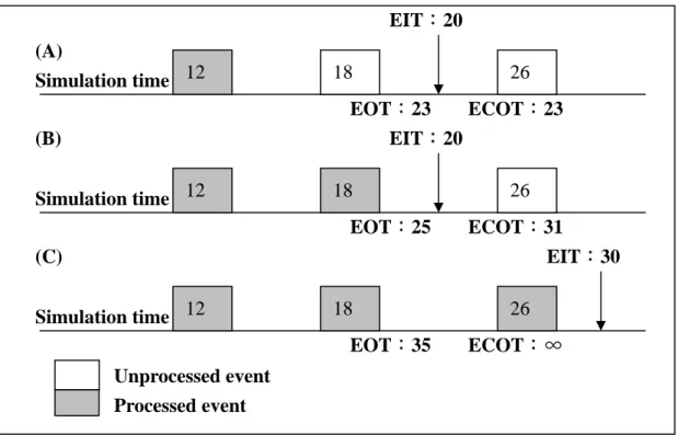
(17) above approaches [21].. Here we cite the definitions and assumptions from the research [22] to simplify the description of below algorithms：. Lookahead (LA)： If a logical process at simulation time T can schedule new events with time stamp of at least T + L, then L is referred as the lookahead for logical process.. Earliest Input Time (EIT)： EIT is a lower bound on the timestamp of any future event message that the logical process may receive.. Earliest Output Time (EOT)： EOT is a lower bound on the timestamp of any future event message that the logical process may send.. Earliest Conditional Output Time (ECOT)： ECOT is a lower bound on the timestamp of any future event message that the logical process may send if logical process will not receive any other messages.. The value of EOT and ECOT for a given logical process depends on its LA, EIT and unprocessed event. Figure 2-1 illustrates the relationship between LA, EIT, EOT and ECOT. We assume the lookahead (LA) in the Figure 2-1 is 5 units. From (A) 7.

(18) scenario in the Figure 2-1, since the timestamp of next unprocessed event is 18 which is smaller the value of EIT 20, the values of both EOT and ECOT are 23, which equal the timestamp of next unprocessed event plus LA, From (B) scenario in the Figure 2-1, the timestamp of next unprocessed event is 26 which is bigger the value of EIT 20, in this condition, the value of EOT is 25 which depends on the value of EIT plus LA, the value of ECOT is 31 which equals the timestamp of next unprocessed event plus LA. From (C) scenario in the Figure 2-1, the value of EOT is 35 because the value of EIT is 30 and there are no unprocessed events, since we expect no known event will happen, the value of ECOT is infinity.. EIT：20 (A) Simulation time 12. 18. 26. EOT：23 ECOT：23 EIT：20. (B) Simulation time 12. 18 EOT：25. (C) Simulation time 12. 18 EOT：35. 26 ECOT：31 EIT：30 26 ECOT：∞. Unprocessed event Processed event Figure 2-1. An example to explain the relation between EIT, EOT, ECOT, LA.. Historically the first synchronization algorithms were based on so-called conservative approaches. The primal conservative synchronization algorithm is presented as pseudo code in Figure 2-2：. 8.

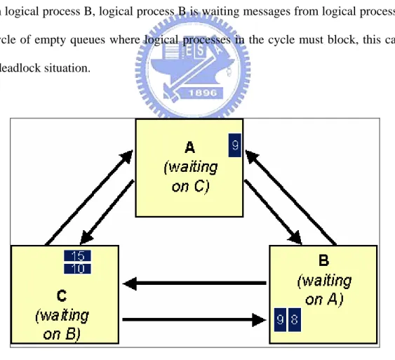
(19) while (simulation is not over) wait until each FIFO contains at least one event remove smallest time stamped event E from its FIFO clock ：= timestamp of event E process the event E Figure 2-2. Initial version of conservative algorithm for a logical process.. As mentioned before, the fundamental problem that conservative mechanisms must solve is to determine when it is “safe” to process an event. Process containing no “safe” events must block, this can lead to deadlock situation if appropriate precautions are not taken. For example, consider the situation of the Figure 2-3, logical process A is waiting messages from logical process C, logical process C is waiting messages from logical process B, logical process B is waiting messages from logical process A. A cycle of empty queues where logical processes in the cycle must block, this cause the deadlock situation.. Figure 2-3. Deadlock situation.. In order to ensure to events are processed in non-decreasing timestamp order and 9.

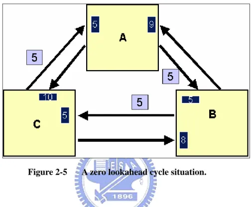
(20) avoid deadlock situation, we discuss below algorithms.. 2.2.1. Null Message Algorithm. The most representative of these kind algorithms is Chandy-Misra-Bryant null message algorithm [18]. The basic idea is that each logical process exchanges its local information to neighbor logical processes periodically in asynchronous manner for synchronization purpose without requiring global synchronization computation. The CMB null message algorithm is presented as pseudo code in Figure 2-4：. while (simulation is not over) // for each LP wait until each FIFO contains at least one event remove smallest time stamped event E from its FIFO clock ：= timestamp of event E process the event E send null messages to neighbor LPs with EOT timestamp Figure 2-4. CMB null message algorithm.. Null messages can be used for a logical process to indicate to other logical processes a lower bound on the timestamp of messages it will send in the future. These messages can update the clock of logical processes to avoid the deadlock situation.. Notwithstanding the famous algorithm works, it still has some problems. One problem is that if there is a zero lookahead cycle (i.e. all lookaheads between links in the cycle are zero). As show in Figure 2-5, although logical process A has processed the event with timestamp 5, simulation time can’t be advanced no matter how many 10.

(21) rounds of null messages LPs had past through, this is because timestamps of all null messages are the same, an un-ending cycle of null messages where no logical processes can advance its simulation time, a livelock happens.. Figure 2-5. A zero lookahead cycle situation.. Another is time creep problem that cause by tiny lookahead value. For instance, if the value of lookahead is one percent of the original, it will takes 100 times of synchronization overhead by a large number of null messages to get the same advance of simulation time, it affects the performance of parallel simulation deeply. The preceding example illustrates a important point：The performance of the null message algorithm depends critically on the lookahead value.. The above two problems can be solved by using global synchronization computation. Global synchronization computation can get the minimum timestamp of events in entire simulation system to break the deadlock situation or speed up the advance of simulation time. The algorithm still has an implicit problem, the synchronization overhead is too heavy because of too many null messages are 11.

(22) transmitted between logical processes. The frequency of null messages sends can have a large effect on performance. The performance is decreasing with an excessive number of null messages.. In order to minimize the number of null messages, one can use the variant of the CMB null message algorithm called lazy CMB null message algorithm. Specifically, null messages are sent when all events have processed before the value of EIT in the logical process. This has the advantage that plenty of null messages are saved because only one null message is sent during each update EIT. The algorithm has implemented to apply the parallel discrete event simulation on NCTUns.. 2.2.2. Conditional Event Algorithm. In the conditional event algorithm, all logical processes are repeatedly cycle through “phases” of （1）synchronization computation for updating EIT value and （2） at least one logical process processing simulation events. In the phase （1）, the state of logical process is blocked until the value of EIT is updated. In the phase （2）, events whose timestamp before the value of EIT are processed by logical process. The mechanism can work without lookahead.. We first consider the synchronous version of the conditional event algorithm. The synchronous mechanism is similar to the barrier synchronization [18, 23]. The value of EIT can treat as the barrier primitive of barrier synchronization. When logical process reach the EIT, it blocks and returns the state to the phase （1）. The value of EIT in the phase （1）is updated to the minimum of ECOT over all logical processes, 12.

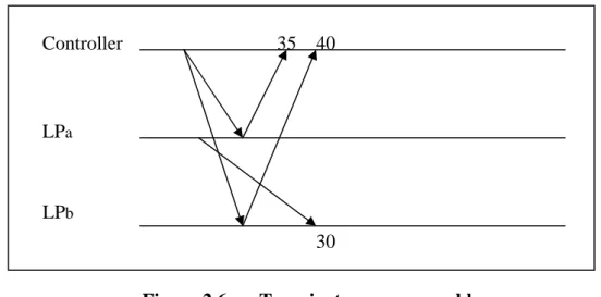
(23) when all logical processes have reached the EIT, each logical process is then allowed to resume simulation. In addition to computing a global minimum, this algorithm must account for messages that have been sent, but have not yet been received, i.e., transient messages. A scenario illustrating the transient messages problem is depicted in Figure 2.6. Logical process LPa and LPb compute their local minimums to be 35 and 40, respectively. If the transit message is not considered, the algorithm will be incorrectly computed as 40, when it should be 30. One simple solution to the transient message problem is to use message acknowledgments that is describing in Global Virtual Time（GVT） computation algorithms [24].. Controller. 35. 40. LPa. LPb 30 Figure 2.6. Transient messages problem.. An asynchronous algorithm allows the value of EIT to be computed without the need to freeze the computation of other logical processes. In order to recover the transient message problem, the definition of EIT in asynchronous mechanism is different from the synchronous one. As shown in Figure 2.7, the value of EIT here is the minimum of all ECOT values of all logical processes and the timestamps of all the messages in transit from all logical processes. The asynchronous approach is similar to a variation of Mattern’s GVT algorithm [25].. 13.

(24) EIT = min { ECOTmin, Msgmin} ECOTmin： the minimum ECOT values of all logical processes Msgmin： the minimum timestamp of messages in transit. Figure 2.7. The definition of EIT in asynchronous conditional event algorithm.. As the value of EIT is computed as minimum of all ECOT values around logical processes, one can improve the performance is that EIT equals to the minimum of global ECOT added with lookahead. The performance of conditional approach depends on the density of events in simulation. It gets better performance than the null message algorithm while in simulation with low density of events and lookahead, vice versa. This topic will be discussed later. Both synchronous and asynchronous approaches of conditional event algorithm has implemented on NCTUns network simulator.. 2.2.3. Accelerated Null Message Algorithm. The accelerated null message algorithm combines the asynchronous null message algorithm with the asynchronous conditional event algorithm. Since events whose timestamp before the EIT value of asynchronous null message algorithm and the EIT value of asynchronous conditional event algorithm are safe to process, the value of EIT in accelerated null message algorithm is computed as the maximum value of two above algorithms.. The motivation of this algorithm is to speed up the computation of EIT by. 14.

(25) asynchronous conditional event algorithm with low lookahead, even without lookahead. In simulation with poor lookahead, the null message algorithm takes a lot of round of null messages that cause the time creep problem. In worst case, the deadlock is arisen by zero lookahead. The advantage of this approach is that it adapt to all kinds of situation. It takes efficiency of null message algorithm while the value of lookahead is not bad, and it also has virtue of the asynchronous conditional event algorithm to execute even without lookahead. While it combines two algorithms, the synchronization overhead is more than others slightly. The topic will be discussed later. The algorithm is implemented as the default synchronization approach on NCTUns network simulator.. 15.

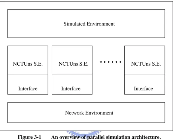
(26) 3. Design and Implementation. This chapter introduces how we apply the parallel discrete event simulation to the NCTUns network simulator, and the detail of the modification for the original sequential simulation engine. In section 3.1, we first introduce the overview of the system architecture. In section 3.2, we describe our modification for the simulation engine of NCTUns. In section 3.3, we next show the required modifications of several protocol modules in NCTUns. In section 3.4, we depict our modification for the Linux kernel in NCTUns.. 3.1. System Architecture Overview. For the parallel discrete event simulation of the NCTUns network simulator, each logical process is actually a simulation engine of NCTUns. Every simulation engine is executed without the support of GUI program in the parallel discrete event simulation mode. Each simulation engine for a parallel simulation is given a simulated environment just the same as one for a sequential discrete event simulation. As such, the modifications to the components in NCTUns can be minimized.. As shown in Figure 3-1, each simulation engine is associated with a network interface to exchange control messages and events that should be simulated by remote simulation engines.. All simulation engines are fed with the same simulation. environment and work cooperatively for the simulation case. In other words, each simulation engine will initialize necessary data structures for each node in a simulated 16.

(27) network despite that the simulation of the node is assigned to a remote simulation engine. However, a simulation engine will not fork traffic generators for a node if the simulation of this node is not assigned to it.. Simulated Environment. NCTUns S.E.. Interface. NCTUns S.E.. ……. Interface. NCTUns S.E.. Interface. Network Environment. Figure 3-1. An overview of parallel simulation architecture.. For a simulation engine, the given simulated environment can be divided into two categories: the global knowledge and the local knowledge. The global knowledge includes the whole simulated network topology, all required routing entries during the simulation, the moving paths of mobile nodes, and several necessary modules for constructing a remote simulated node. The local knowledge includes the detailed information of all modules for nodes that are going to be simulated on the local machine. Since a simulation engine only needs to keep the detailed information for its own local simulated nodes, the engine can save memory space by constructing its local simulated nodes with all required module objects and constructing remote. 17.

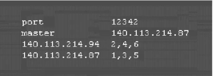
(28) simulated nodes with minimized numbers of module objects.. The only difference at the initial stage between the parallel simulation and the original one is that we need to configure the “parallel.cfg” file for each simulation engine before starting a simulation in the parallel mode. The “parallel.cfg” file specifies the partition for this simulated network. The format of the “parallel.cfg” file is shown in the following in sequence.（1） the control port for all participants in the simulation case, （2）the IP address of the master simulation engine in the simulation case, （3）the IP address of the local simulation engine and its local simulated nodes, and （4） the IP address(es) of other remote simulation engine(s) and its (their) own local simulated nodes. As the example illustrated in Figure 3-2, the control port number is 12342. The IP address of the master simulation engine is 140.113.214.87, and the IP address of local simulation engine is 140.113.214.94.. The local. simulation engine is in charge of nodes 2, 4, 6 in this simulation. Since its IP address is different with the master one, this local simulation engine is one of the slave simulation engines in this simulation. The IP address of the other simulation engine, which is responsible for nodes 1, 3, 5, is 140.113.214.87. Since this simulation engine has the same IP address as the master, it is actually the master simulation engine for this simulation.. Figure 3-2. An example of configuration in the “parallel.cfg” file.. 18.

(29) The partition of a simulated network in NCTUns is on the node basis rather than the geometric basis. As mentioned in paper [2], the NCTUns network simulator uses the real-life Linux TCP/IP protocol stack. Real-world user-level applications can be run directly on top of it. As such, suppose we partition the network into several geometric areas. While a mobile node moves across at least two areas, it is arduous to switch a user-level process running on the simulated mobile node from one machine to another because transferring a user-level process includes several difficult tasks. For example, we need to transfer the contents of the process’s memory pages and several data structures in the kernel for this process to a remote machine.. Besides applying conservative algorithms to original one, there are some problems that need to be dealt with. For example, we need a way to make a kernel know that the simulation will be executed in the parallel mode or the single mode. In addition, the mapping scheme for virtual and physical ports is important in NCTUns. How to map virtual and physical ports for different kernels on several distributed computers is not an easy task. Moreover, configuring the settings for modules of non-local nodes (i.e. nodes simulated by remote simulation engines) requires an additional mechanism. We discuss these implementation issues in the following sections.. 3.2. Simulation Engine Modification. This section describes the modification of the NCTUns simulation engine for the parallel discrete event simulation. The operations of the kernel in the parallel simulation mode are different from those in the single machine mode, so a simulation 19.

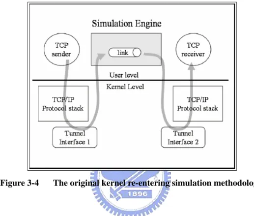
(30) engine needs a way to make kernel know in which mode it has to run. We achieve this by altering two system calls shown in Figure 3-3.. syscall(275, 0x0c, 0, 0, 0);. // Let kernel node S.E. are in parallel/distributed mode.. syscall(275, 0x0d, 0, 0, 0);. // Reset the parameter “parallel_mode”.. Figure 3-3. The hacked system call to set parallel/single mode in kernel.. The detail of a simulation executed on a single machine is explained on [27]. The basic idea is shown in Figure 3-4. The TCP/IP protocol stack used in the simulation is an existing real-life one in the kernel. Although each node thinks that it has its own protocol stack, all simulated nodes actually have the same protocol stack because they are all run on a single machine. The tunnel interfaces shown in the Figure are pseudo network interfaces that do not have a real physical network attached to it. However, from the kernel’s point of view a tunnel interface is not different from any real Ethernet network interfaces.. In Figure 3-4, the TCP sender sends a packet into the kernel, and the packet goes through the kernel’s TCP/IP protocol stack just as an Ethernet packet would do. Because we configure the tunnel interface 1 as the packet’s output device, the packet will be inserted to tunnel interface 1’s output queue. The simulation engine will immediately detect such an event and issue a read system call to get this packet through tunnel interface 1’s special file (Every tunnel interface has a corresponding device special file in the /dev directory.). After experiencing the simulation of transmission delay and link’s propagation delay, the simulation engine will issue a write system call to put the packet into tunnel interface 2’s input queue. The kernel will then raise a software interrupt and put the packet into the TCP/IP protocol stack. 20.

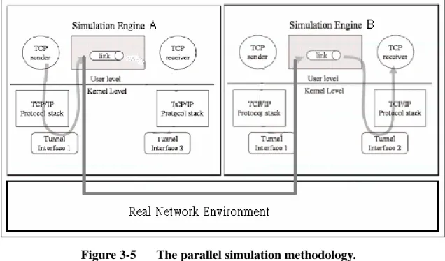
(31) Then, the packet will be put into the receive queue of the socket that the TCP receiver creates. Finally, the TCP receiver will use a read system call to get packet out of the kernel.. Figure 3-4. The original kernel re-entering simulation methodology.. In Figure 3-5, we illustrate how several parallel/distributed simulation engines cooperate to complete a simulation. The simulation engines A and B have the same information for the simulated network, but each of both only simulates a portion of the network. The TCP sender is simulated on the simulation engine A, and the TCP receiver is simulated on the simulation engine B. As illustrated in Figure 3-4, when a packet is sent out from the TCP sender, it will be captured by the simulation engine A before it is inserted into the simulation engine’s event list. The simulation engine A first checks if the destination node of this packet is simulated is a local simulated node or a remote simulated node. The simulation engine A regards a simulated node as a local node if this node is simulated on the simulate engine A itself. Otherwise, the simulation engine A regards a simulated node as a remote node. Next, the simulation 21.

(32) engine A obtains the node ID of the destination node for this remote packet via the “get_nid()” NCTUns API call. The “get_nid()” NCTUns API call is a primitive function call provided by the simulation engine. This function call works well in our parallel simulation environment because, as mentioned previously, each simulation engine creates all simulated nodes with at least necessary data structures and thus the node list of each simulation engine includes the information for all simulated nodes. As such, even if the “get_nid()” call is for a remote node, it still succeed in returning the correct node ID for that remote node.. Figure 3-5. The parallel simulation methodology.. Then, the simulation engine looks up the “parallel.cfg” file to know which remote simulation engine is responsible for the simulation of the destination node. Afterwards, the simulation engine A encapsulates this simulated packet into a specific event format defined in the “parallel.h” header file and passes the encapsulated event to the simulation engine B through the underlying real network. The simulation engine B inserts this remote event into its own event list upon its receiving this remote 22.

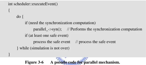
(33) event. Finally, the TCP receiver on the machine of the simulation engine B will receive this simulated packet sent from the TCP sender on the machine of A.. User-level traffic generators are executed on top of a simulation engine. A simulation engine is not allowed to execute traffic generators belonging to non-local nodes to make sure the behaviors of user-level application programs are correct. We achieve this by modifying the “read_trafficGen()” function in the “event.cc” file.. int scheduler::executeEvent() { do { if (need the synchronization computation) parallel_->syn(); // Performs the synchronization computation if (at least one safe event) process the safe event // process the safe event } while (simulation is not over) } Figure 3-6. A pseudo code for parallel mechanism.. In the parallel simulation, all simulation engines repeatedly cycles of two phases, “synchronization” and “event processing”. We modified the “scheduler” component, defined in the “scheduler.cc” file, in the simulation engine based on the pseudo code shown in Figure 3-6. In the synchronization phase, a simulation engine gets the value of EIT. In the event processing phase, a simulation engine is allowed to process the safe events, the timestamps of which are before EIT.. 3.3. Modules Modification. 23.

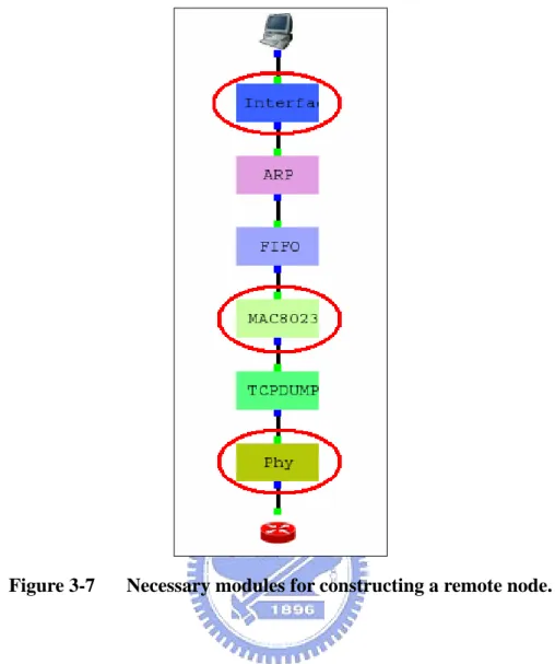
(34) In the parallel simulation, each simulation engine only needs to simulate a portion of a simulated network. Since the NCTUns network simulator uses the kernel re-entering simulation methodology, each simulated node has to make kernel know some necessary information such as the MAC addresses, the IP addresses and the the netmasks of interfaces that will be simulated on tunnel interfaces. For this reason, we alter the “tclObject.cc” file to modify the node construction process because several modules in remote nodes (i.e. nodes are simulated on other remote simulation engines) still need to be constructed. We show those necessary modules for constructing a remote node as shown in Figure 3-7 and explain why they are necessary for a remote node.. Interface module： An interface module is required for keeping the IP address and the netmask of a remote node for a local kernel.. MAC relative (802.3, 802.11) modules： A MAC-layer module is required for storing the MAC address of a remote node for a local kernel.. LINK and PHY relative (phy, ophy, wphy, awphy) modules： Link and PHY-layer modules are required to describe the connectivity of the whole network so that a remote packet can be inserted to a correct physical module when this packet arrives at the proper remote simulation engine.. 24.

(35) Figure 3-7. Necessary modules for constructing a remote node.. 3.4. Kernel Modification. This section describes the detail of modification in kernel to apply the parallel discrete event simulation to the NCTUns network simulator.. We add a new global parameter, “parallel_mode”, into the kernel to make the kernel know that the simulation will be run in the parallel mode or in the single mode. The simulation engine can use the modified system to alter the value of the “parallel_mode” parameter as shown in Figure 3-8.. 25.

(36) /* system call 275 in 2.6 kernel*/ asmlinkage int sys_NCTUNS_misc(…) { … case 0x0c: parallel_mode = 1; // run into parallel mode break; case 0x0d: parallel_mode = 0; break; } Figure 3-8. The system call to change the state of “parallel_mode” parameter.. Since NCTUns uses the port-mapping mechanism [26, 27] in kernel with the real-life TCP/IP protocol stack, those original mechanisms that are related to data structures of the kernel may introduce several problems for the parallel discrete event simulation. For instance, suppose that the virtual port number of the TCP sender on the node A is 6000 and the corresponding real port number is 5001. The virtual port number of the TCP receiver on node B is 5001 and the corresponding real port number is 5002. When the TCP receiver on node B receives a packet transmitted by the TCP sender on the node A, it should send an ACK packet back to the TCP sender. In the single mode, it can be done simply by looking up the “mtable” data structure in the kernel to get the virtual port number of the TCP sender. Then it sends the ACK packet with 6000 as the destination port number, as shown in Figure 3-9. If we want to use the parallel simulation scheme to simulate the above simulation case, the TCP sender of the node A will be executed on one machine and the TCP receiver of node B will be executed on another. Since the kernel of each machine only knows the information of its own data structures, the information of the port mapping for all simulated nodes is not easy known by the kernels of all simulation machines.. 26.

(37) Figure 3-9. An example of “mtable” data structure.. To address this problem, we changed the “tun0event” structure in the “nctuns_t0e.h” file shown in Figure 3-10. First, we observed that all user-level network application programs invoke the “bind()” system. Since the “bind” system call will issue the mt_bind() function in the kernel, we add the “tun0_port()” function into the “mb_bind()” function. The “tun0_port0” function is fed with a node ID N, a real port number Rp, and a virtual port number Vp. This function sets a tun0-event (a special control for the communication between the NCTUns simulation engine and the kernel) with an entry specified by (N, Rp, Vp) in the “mtable” structure (the port mapping table). Then the “tun0_port()” function puts this tun0-event to the tun0 interface. The simulation engine then catches the tun0-event and sends the event to other remote simulation engines. When a remote simulation engine receives such an event, it will issue a hacked system call to invoke the “mt_port_add()” function in the kernel. The “mt_port_add()” function then adds entries contained in this tun0-event into the “mtable” data structure of this remote machine. In such a way, the kernels of 27.

(38) all simulation machines are capable of knowing the port-mapping for all simulated nodes.. struct tun0event { int int u_int32_t unsigned short unsigned short }; #define T0E_TIMEOUT #define T0E_CHKTUN #define T0E_PORT_ADD. pid; flag; value; rport; vport;. // for parallel simulation // for parallel simulation. 1 2 3. // for parallel simulation. #define T0E_PORT_DEL 4. // for parallel simulation. Figure 3-10. The modification of tun0event structure.. 28.

(39) 4. Performance Evaluation. In this chapter, we examine the performances of some parallel conservative algorithms. Next, we compare the performances of parallel simulations between two popular network simulators, NCTUns and NS2. Finally, we discuss the effects of several important factors in parallel simulation.. Before we explain the performance results, we fist define our performance metrics, the “speedup” and “event-processing rate”. The definitions of these metrics are as follows.. Speedup. ＝. Sequential Execution Time —————————————— Parallel Execution Time. Event-Processing Rate ＝. Total Events in Simulation —————————————— Execution Time. 4.1. Conservative Algorithms Comparison. In this section, we first observe the influence of lookahead value on different conservative algorithms. Then, we study the performances in terms of the metrics, the execution, the speedup and the event-processing rate, respectively.. 29.

(40) 4.1.1. Conservative Algorithms Comparison By Lookahead In this section, we illustrate the influence of lookahead values with two examples. In the first one, we show the effect of a large lookahead value, and in the second one we show the effect introduced by a small lookahead value.. The simulation network for the first case is partitioned into two parts, each of which is assigned a simulation engine. As shown in Figure 4-1, one simulation engine is in charge of the simulation of nodes 1, 2, 4, 5, 6, 7, 8, 9, 10, and the other is responsible for the simulation of nodes 3, 11, 12, 13, 14, 15, 6, 17, 18. There are three TCP connections in this simulation case, each of which is from node 18 to node 5, from node11 to node 6, from node16 to node10, respectively. The lookahead value (i.e. the propagation delay) for this case is 10,000 microseconds.. Figure 4-1. Example 1 for conservative algorithms comparison.. The execution times of algorithms are shown in Table 4-1. Since the lookahead value is large, in all conservative algorithms, the execution time of the null message 30.

(41) algorithm is the best and most close to the sequential one. The accelerated null message algorithm also makes use of large lookahead value to shorten its execution time. The execution time of the conditional event algorithm is the worst. This is because it is not able to take advantage of a large lookahead value.. Approach Sequential Time (sec). Null Message. Conditional. Execution. Algorithm. Event Algorithm Message Algorithm. 7.299. 7.977. Execution time. 27.105. Accelerated Null. 11.85. Table 4-1 Execution time of conservative algorithms （1）.. We next discuss the second case, in which the used lookahead value is much smaller than that in the first case. The simulation network for the second case is also partitioned into two parts, and each part is assigned a distinct simulation engine. As shown in Figure 4-2, one simulation engine is in charge of the simulation of node 1, and the other is in charge of the simulation of node2. There is a UDP data steam from node 1 to node 2 in this 802.11 wireless network. The average of lookahead values (i.e. signal propagation delay) is about 5 microseconds.. Figure 4-2. Example 2 for conservative algorithms comparison. 31.

(42) The execution times of the algorithms in the second case are shown in Table 4-2. Such small values of the lookahead cause that the performance of the null message algorithm becomes extreme low. The performances of both the accelerated null message algorithm and the conditional event algorithm are much better than those of the null message algorithm since the global minimum ECOT interval is larger than the values of lookahead.. Approach Sequential Time (sec). Execution. Execution time. 3.91. Null Message. Conditional. Algorithm. Event Algorithm Message Algorithm. 1454.11. Accelerated Null. 37.105. 34.98. Table4-2 Execution time of conservative algorithms （2）.. The above execution time results show that the lookahead value is an important factor that influences the performance of both the null message algorithm and the accelerated null message algorithm. They also show that if the number of total events to be simulated is relatively small, the overheads for synchronizing simulation engines will become a large portion for the total simulation time. For this reason, the performances of conservative approaches are worse than the sequential one in both cases.. 4.1.2. Conservative Algorithms Comparison By Event-Processing Rate and Speedup. In this section, we evaluate the performances of conservative algorithms using. 32.

(43) event-processing rate and speedup as the metrics of comparison. The simulation network topology is shown in Figure 4-3. There are two UDP CBR (constant bit rate traffic pattern) data streams in this case, each of which is from node1 to node 3, from node 2 to node 4, respectively. We conducted the simulation of this case with two different traffic patterns for the two UDP CBR data streams. In the first one, these two streams send a packet of length 128 bytes at a time with 0.1 milliseconds, and thus the resulting data rate of each UDP stream is 10Mbps. In the second one, the two data UDP streams send a packet of length 1024 bytes with the period of 0.8 milliseconds. Thus, the resulting data rates of these UDP streams are also 10 Mbps. Note that although the two traffic patterns generate the same data rates, they generate different numbers of events. The given lookahead values for these two cases are 10, 1000, and 100000 microseconds, respectively. In these cases, the bandwidths of all links are 1000 Mbps, and the simulation time of each case is 30 seconds (in terms of virtual time). The simulation topology is partitioned into two parts, each of which is assigned a simulation engine. One simulation engine is responsible for the simulation of the nodes 1, 2, 5. And the other is responsible for the simulation of the nodes 3, 4, 6.. Figure 4-3. A simulation case for conservative algorithms comparison.. 33.

(44) The simulation results are shown in Figure 4-4. As the lookahead value increases, the event-processing rate of the sequential simulation decreases. This is a heartening observation because the larger the lookahead value is, the better the parallel discrete event simulation performs. The event-processing rate of the null message algorithm is similar to the accelerated null message algorithm since the given lookahead values are sufficiently large. The event-processing rate is direct proportional to the lookahead value in the conservative algorithms. That is, if the value of the lookahead decreases, the event-processing rates of those conservative algorithms will decrease as well. In addition, if the lookahead value is so small, the null message algorithm will suffer form the “time creep problem.” The main reason that other conservative algorithms perform poorly in this series of simulations is that the transmission rates of UDP streams is too high to make these algorithms due to synchronization overheads. However, if the lookahead value is sufficiently large, the conditional event algorithm results in the worst event-processing rate compared with other algorithms. The above observations show that the lookahead value is the most important factor for the performances of PDES.. Figure 4-4. Event-Processing Rate with logging statistics. 34.

(45) Since the logging action requires many I/O operations, it influences the event-processing rate a lot. The event-processing rate without logging statistics is approximately double than that with logging statistics. The result of the event-processing rate without logging statistics is shown in Figure 4-5. The observations derived from Figure 4-5 are similar to those derived from Figure 4-4.. Figure 4-5. Event-Processing Rate without logging statistics.. The speedups of conservative algorithms with the 10Mbps (0.1 ms x 128 bytes) traffic pattern are shown in Figure 4-6. The speedups of all conservative algorithms are disappointing while the value of lookahead is 10 microseconds. The speedup of the null message algorithm is similar to the speedup of the accelerated null message algorithm. Furthermore, both algorithms get better performances while the lookahead value increases. It is evident that the speedup of conditional event algorithm is worse than those of others.. The speedups of conservative algorithms with the 10Mbps (0.8ms x 1024 bytes) traffic pattern are shown in Figure 4-7. The speedup result shows that the speedups of 35.

(46) 10 Mbps ( 1 ms x 128 Bytes ). Speedup. 1.5. Condional event with LOG Accelerated null msg with LOG. 1. Null msg with LOG. 0.5. Condional event without LOG. 0 10. 1000. 100000. Lookahead (microsecond). Figure 4-6. Accelerated null msg without LOG Null msg without LOG. Speedup – 10 Mbps (0.1 millisecond x 128 bytes).. conservative algorithms increase as the value of lookahead increases. When the lookahead value is 10000 microseconds, both the null message algorithm (with logging statistics) and the accelerated null message algorithm (with logging statistics) have more speedup values by one than the speedup values using 10 microseconds as the lookahead value.. 10 Mbps ( 8 ms x 1024 bytes ). Speedup. 1.5. Accelerated null msg with LOG. 1. Null msg with LOG. 0.5. Conditional event without LOG. 0 10. 1000. 100000. Lookahead (microsecond). Figure 4-7. Conditional event with LOG. Accelerated null msg without LOG Null msg without LOG. Speedup – 10 Mbps (0.8 milliseconds x 1024 bytes).. 36.

(47) Comparing Figure 4-6 with Figure 4-7, we can find that increasing ratios of the speedups are different with different traffic patterns. For the segments in terms of the lookahead values from 10 to 1000 microseconds, the speedup with the traffic pattern (0.1 ms x 128 bytes) increases more than the speedup with the traffic pattern (0.8 ms x 1024 bytes). This is because the traffic pattern in Figure 4-6 generates more events than the traffic pattern in Figure 4-7 does. The simulation engines in Figure 4-6 can process more events to achieve better speedup within the same lookahead interval. For the segments in terms of the lookahead values from 1000 to 100000 microseconds, the speedup with the high event-number traffic pattern is smoother than that with low event-number traffic pattern. This is because the number of events that can be processed is gradually saturated as the value of the lookahead increasingly increases.. 4.2. Simulator Comparison. In this section, we compare the performances of parallel simulations for two popular network simulators, NCTUns and NS2. PDNS (parallel/distributed NS2) [28, 29, 30] is developed by the PADS research group at Georgia Tech. The simulation case used in this section is the same as the one used in Figure 4-3.. The event-processing rate of the original sequential execution on NS2 is shown in Figure 4-8. It shows that the event-processing rate increases as the number of events increases. The event-processing rate without additional logging I/O overheads is much faster than one with logging statistics. In other words, the bottleneck of the event-processing rate on NS2 is the logging mechanism.. 37.

(48) 10 Mbps (1 ms x 128 bytes) with LOG. event processing rate (events/execution time). 1000000 800000. 10 Mbps (1 ms x 128 bytes) without LOG. 600000 400000. 10 Mbps (8 ms x 1024 bytes) with LOG. 200000 0 10. 1000. 100000. lookahead (microsecond). Figure 4-8. 10 Mbps (8 ms x 1024 bytes) without LOG. Event-Processing Rate on PDNS.. From Figures 4-4, 4-5, and 4-8, the event-processing rate with additional logging I/O overheads on NCTUns nearly equals to the event-processing rate with logging overheads on NS2, since both of them are limited by disk I/O operations. On the contrary, the event-processing rate without logging statistics on NCTUns is much less than that without logging statistics on NS2.. We compare the speedups on NCTUns with the speedups in PDNS. As shown in Figure 4-9 and Figure 4-10, the overall behaviors of the speedups on NCTUns are similar to those on PDNS. The event-processing rate without logging I/O overheads on PDNS is much faster than that with logging I/O overheads. In contrast to NS2, the event-processing rate without logging statistics on NCTUns is only two times faster than the one with logging overheads. The maximum speedup on PDNS is close to 1.4, and that on NCTUns is close to 1.2. The reason is that packets in PDNS are transmitted in a pseudo way. In other words, packets in transit are simulated by transmitting a small descriptor that contains the information such as the packet length rather than transmitting a real packet. Contrarily, packets transmitted on NCTUns are 38.

(49) real ones because NCTUns uses the real-life TCP/IP protocol stack, which may produce the additional transmission delay in the parallel/distributed simulation. speedup (Sequential/Accelerated null message). environment.. 10 Mbps (1 ms x 128 bytes) with LOG. 1.2 1. 10 Mbps (1 ms x 128 bytes) without LOG. 0.8 0.6 0.4. 10 Mbps (8 ms x 1024 bytes) with LOG. 0.2 0 10. 1000. 100000. lookahead (microsecond). Speedup(sequential/accelerated null message). Figure 4-9. 10 Mbps (8 ms x 1024 bytes) without LOG. Speedup on NCTUns.. 10 Mbps (1ms x 128 bytes) with LOG. 1.6 1.4 1.2 1 0.8 0.6 0.4 0.2 0. 10 Mbps (1 ms x 128 bytes) without LOG 10 Mbps (8 ms x 1024 bytes) with LOG 10. 1000. 100000. lookahead (microsecond). Figure 4-10. 10 Mbps (8 ms x 1024 bytes) without LOG. Speedup on PDNS.. The differences of functionality between NCTUns and PDNS are shown in Table 4-3. 39.

(50) Approach Partitioning. NCTUns. PDNS. Custom Design. Federated Approach. Partitioning can occur Partitioning can only occur between any type of nodes between routers. Routing. Automatically done. Need to set up in TCL. Setup. Use “parallel.cfg” to. Need to use new TCL. partition network. syntax. Support. No Support. Wireless Simulation Table 4-3. Functionalities between NCTUns and PDNS.. 4.3. The Impact Factors for Parallel Simulation. In this section, we discuss the effects of several factors in parallel simulation including lookahead, connectivity between simulation engines and load balance.. The simulation network topology is shown in Figure 4-11. There are four UDP CBR (constant bit rate traffic pattern) data streams in the simulation case, two-way on from node 1(3) to node 3(1), from node 2(4) to node 4(2), respectively. These four streams send a packet of length 128 bytes at a time with 0.1 milliseconds, and thus the resulting data rates of the UDP streams are 10Mbps. The bandwidths of all links are 1000 Mbps, and the simulation time in the case is 10 seconds (in terms of virtual time). The simulation topology is partitioned into two parts, each of which is assigned a simulation engine. One simulation engine is responsible for the simulation of the nodes 1, 2, 5. And the other is responsible for the simulation of the nodes 3, 4, 6.. 40.

(51) Figure 4-11. A simulation case for impact factors.. 4.3.1. Lookahead. In this section, we discuss the lookahead, which is the most important factor for parallel simulation.. The execution times of different lookahead values are shown in Figure 4-12. It is observed that if the value of lookahead is 10 microseconds, it will be the bottleneck let all execution times of conservative algorithms become extremely long. The execution time is following the lookahead value to increase on original sequential simulation. The curves of both the null message algorithm and the accelerated null message algorithm looks alike and have less execution time than sequential one while the lookahead value is larger than 100 microseconds. The execution times of the conditional event algorithm are longer than sequential one whichever the lookahead value is.. 41.

(52) Execution time (sec). Null message. Accelerated null message. Conditional event. Sequential. 200 150 100 50 0 10. 100. 1000. 10000. 100000. Lookahead (microsecond). Event processing rate (events/execution time). Figure 4-12. Execution times for different lookahead values.. Null message. Accelerated null message. Conditional event. Sequential. 50000 40000 30000 20000 10000 0 10. 100. 1000. 10000. 100000. Lookahead (microsecond). Figure 4-13. Event processing rate for different lookahead values.. The event-processing rates of different lookahead values are shown in Figure 4-13. As the lookahead values increase, the event-processing rates of sequential execution follow to decrease progressively. The event-processing rate of the conditional event algorithm is not well no matter what lookahead value is. The curves of both the null message algorithm and the accelerated null message algorithm look alike and have higher event-processing rate than the sequential execution one while 42.

(53) the lookahead value is 100000 microseconds.. Null message Accelerated null message Conditional event. Speedup (Sequential/Parall el). Speedup 2.5 2 1.5 1 0.5 0 10. 100. 1000. 10000. 100000. Lookahead (microsecond). Figure 4-14. Speedups for different lookahead values.. The speedups of different lookahead values are shown in Figure 4-14. The speedups of conservative algorithms are following the lookahead values to increase. We take notice of both the speedups of the null message algorithm and the accelerated null message algorithm that larger than 2, while the lookahead value is 100000 microseconds. Figure 4-14 shows that the execution times of both algorithms are almost the same while the lookahead values are in range from 100 to 100000 microseconds in Figure 4-12. Since the execution times are almost the same, the reason that cause the speedup larger than 2 is that the execution time of the sequential execution is in increasing. This is because as the lookahead value increases, the event-processing rate of the original sequential execution decreases progressively, as shown in Figure 4-13.. 43.

(54) 4.3.2. Connectivity between Simulation Engines. In this section, we discuss the connectivity between simulation engines, a factor influence the performance of parallel simulation. We change the partition in Figure 4-11 as shown in Figure 4-15. We split up the simulation into two simulation engines. One is in charge of the nodes 1, 3, 5, and the other is in charge of the nodes 2, 4, 6. We test the simulation case with the null message algorithm. Figure 4-15. Partitioning for connectivity between simulation engines.. The partition of simulated network in the case will cause additional 200,002 remote send packet events and 200,002 remote receive packet events on different simulation engines. The large number of additional packet transmission overhead of these remote packet events transmitted on real network, will cause about half speedup as shown in Figure 4-16.. 44.

(55) Speedup (execution time of null message algorithm / execution time of remote packet partition). Speedup. 0.6 0.4 0.2 0 10. 100. 1000. 10000. Lookahead (microsecond). Figure 4-16. The speedup under the partition of connectivity between simulation engines.. 4.3.3. Load Balance. In this section, we discuss the load balance, a factor influence the performance of parallel simulation. We change the partition in Figure 4-15 as shown in Figure 4-17. We split up the simulation into two simulation engines. One is in charge of the nodes 1, 2, 3, 5; the other is in charge of the nodes 4, 6. We test the case with null message algorithm.. The partition of network causes additional 100,001 remote send packet events and 100,001 remote receive packet events. Compared with the partition in Figure 4-15, although this partition in Figure 4-17 has only half number of remote packet events, but its performance is worse than the other. This is because the workload of assignment is not uniform for each simulation engine. In this case, the simulation engine in charge of the nodes 1, 2, 3, 5, is busy with heavy workload and the 45.

(56) simulation engine in charge of the nodes 4, 5 is idle in most time to wait synchronization with the other simulation engine. The speedup is getting worse with smaller lookahead value since tiny lookahead value cause large synchronization overhead as shown in Figure 4-18.. Figure 4-17. Partitioning for load balance.. Speedup (execution time of remote packet partition / execution of load balance partition). Speedup. 1.5 0.95713841. 1 0.5. 0.038398159. 0.255943618. 0 10. 100. 1000. Lookahead (microsecond). Figure 4-18. The Speedup under the partition of load balance.. 46.

(57) 5. Future Work. In the future, we intend to implement several algorithms of optimistic approach [18] on NCTUns network simulator to evaluate the performance of optimistic algorithms and compare the performances of optimistic approach with the performances of conservative approach.. The performances of parallel discrete event simulation for wireless network simulation are disappointed. The propagation delays of signal transmission in wireless network are tiny. These so small look-ahead values make the parallel discrete event simulation perform inefficiently. However, one can increase the lookahead values from the logical processes by the nature of the CSMA/CA protocol in IEEE 802.11 wireless networks. The CSMA/CA protocol requests each node in the network to postpone the sending of frames with various periods called “inter-frame space” (IFS), such as SIFS, PIFS, DIFS and EIFS. As such, those idle times due to IFSs are useful for the lookahead of logical processes.. The parallel discrete event simulation still has many challenges. First, partitioning a network topology automatically in a best way is still difficult. So far we leave this task with users. An inappropriate network partition could severely decrease the performances of the parallel discrete event simulation. In the future, we will investigate how to partition a network more wisely.. Second, NCTUns works with the real-life TCP/IP protocol stack collaboratively. This methodology produces more accurate simulation results. 47.

(58) However, it also increases the difficulty for the parallel discrete event simulation. Protocols that involve operating data structures in the kernel may not function correctly in a distributed simulation environment. For example, routing protocols, such as OSPF, RIP, etc, need to operate the kernel’s routing table to build routes correctly. In a distributed simulation environment, these routing daemons are running on different machines. In such a situation, the kernel’s routing table of each machine may not be consistent with each other because each routing daemon is only able to update the routing table on its local machine. To address this problem, we need to propose a new mechanism for the parallel simulation to exchange the contents of kernel data structures when needed. This is a huge task that remains to be completed in the future.. 48.

(59) 6. Conclusion. This thesis presented how conservative synchronization algorithms are applied to NCTUns network simulator with minimum modifications, and therefore most of network protocol modules, existing tools and traffic generators that have been developed can be reused. We study the performance of some conservative synchronization algorithms that have been implemented on NCTUns network simulator, including the asynchronous lazy null message algorithm, the conditional event algorithm and the accelerated null message algorithm. The thesis expands on the limits of packet level simulation using a variety of parallel computation techniques and discusses the impact factors that influence the performance of the parallel discrete event simulation.. This thesis concludes some guidelines to achieve good performances for the parallel simulation. First, the lookahead values should be sufficiently large. This is also the most significant factor for the parallel simulation. Second, making a good partition for a network can reduce the communication overheads between logical processes. Such communication overheads for a logical process include the exchanges of control messages, simulated data packets, and the delays for waiting messages from other logical processes. Third, the density of events (the number of events that should be processed in every second) of a simulation case should be high for the parallel simulation to get better performances than a sequential one. Next, the load balance is important for logical processes, the performance of parallel simulation is decreased by additional waiting time for light-workload logical processes in idle. Finally, it is very important to use a high-throughput and low-delay inter-connection network as the 49.

(60) underlying network system for the parallel simulation. For example, if the used underlying inter-connection network has high-delays for exchanging packets among nodes, logical processes running on these nodes may experience unacceptable message-passing delays, and thus the total execution time for a simulation is increased inevitably.. With respect to conservative synchronization algorithms, the null message algorithm usually has the best performances for the parallel discrete event simulation if the used lookahead values are large sufficiently. The conditional event algorithm has inverse proportion relationship between the efficiency and the density of events. It gets better performances than the null message algorithm while simulation with small lookahead values. The accelerated null message algorithm combines the advantages of the above two algorithms. It often has good performances for all kinds of simulation cases in the parallel discrete event simulation.. 50.