Performance Analysis of an Offshore Gas-Turbine Power System

(1)

Performance Analysis of an Offshore Gas-Turbine Power System

M.-C. Chang, M.-J. Chen, S.-H. Wen and C.-H. Li

Department of Electrical Engineering, National Kaohsiung University of Applied Sciences E-mail: fc4572@ms42.hinet.net

Abstract

The objective of this paper is to analyze the dynamic performance of an offshore gas-turbine power system operating in normal and abnormal situations. The system primarily consisted of two gas-turbine generation systems and other electrical components. The mathematical models for the components, developed to cater for the dynamic behavior of the system using Simulink and SimPowerSystems, included gas-turbine model, electric machine model, electromechanical model, and three-phase power transformer model. The method for predicting the dynamic responses of interconnected machine systems, named dynamic voltage-current combination method, was employed to connect system components in this research. Simulation results show that the system operated satisfactorily in normal and abnormal conditions. The dynamic behavior study for an offshore power system is essential for system planning, operation, and further expansion.

Keywords: Dynamic Behavior, Gas Turbine, Offshore Power System, Mathematical Model, State Space Approach, Dynamic Voltage-Current Combination Method, Simulink, SimPower Systems

1. INTRODUCTION

The offshore oil industry has been well established on the continental shelves for some decades. In that time considerable amount of power generation has been installed on oil and gas production platforms. The sizes of gas turbines and power generators have gradually increased as the electrical load on the platforms has increased.

In the majority of industrial or small system applications, the starting of induction motor is accompanied by a voltage depression and possible frequency variation. The magnitude of these fluctuations is dependent on the size of the motor relative to the generation system and the responses of both the prime-mover system and the automatic voltage regulation system. In order to accurately predict the starting current, torque requirements, and the time taken to reach full speed, the overall simulation model must be capable of allowing for depressions in the supply voltage. The above requirements imply that in addition to the careful attention given to drive system model equal attention is necessary in modeling the generation system including adequate representation of the prime mover.

The approach to modeling gas turbines is similar to that adopted for the diesel engine; in that the characteristic maps representing the performance of the compressor and turbine are generally used to derive the significant features of the responses. The level of complexity of the single shaft

(2)

gas turbine model is also similar to that of the diesel engine since the compressor is operating at essentially constant speed. The response of the single shaft gas turbine to a load change is usually dictated by the dynamics of the governing system rather than the prime mover itself. The basic governing of the gas turbine is similar to that employed for the diesel engine, i.e. droop with load sharing, but includes the effects of turbine temperature to control overloading of the unit.

A number of studies have been conducted on gas turbine power systems. Some of them have been done on the stability of gas turbine power system[1-3], some on the model of gas turbine[4-6], some on the performance of fuel cell-microturbine hybrid system[7-10], some on the application of combined-cycle power system[11-13], and some on other fields such as performance during frequency variation and controller design[14,15]. However, few of them have discussed the dynamic performance of standalone gas turbine power systems.

This paper presents the dynamic performance of an offshore gas-turbine power system operating in normal and abnormal situations. The mathematical models for the components, developed to cater for the dynamic behavior of the system using Simulink and SimPowerSystems, included gas-turbine model, electric machine model, electromechanical model, and three-phase power transformer model. Simulation results show that the system operated satisfactorily in normal and abnormal conditions. This type of study is important in system planning to design required system enhancements, in system operations to establish secure operating limits, and for designing appropriate remedial control and protection schemes to improve the power system response to disturbances.

2. METHODOLOGY OF ANALYSIS

2.1 State Space Approach

The state space technique is generally employed to model power system components by specifying a set of first order differential equations. This method facilitates a modular approach to system modeling, which directly assists in dealing with system of widely varying configuration[16,17].

The differential equations of each item of plant and associated control and that of the overall system are given by

[ ] [ ][ ] [ ][ ]

p X = A X + B U ₍₁₎

where [X] is the n dimensional state vector, [A] is an nxn state coefficient matrix, and p is the differential operand. The system inputs are represented by the m dimensional vector [U] and an nxm control matrix [B].

2.2 Method of Machine Interconnection

In the dynamic current summation method, a synchronous generator is modeled as a current source[18]. However, in this combined method, called dynamic voltage-current combination method, a synchronous generator is treated not only as a current source but also as a voltage

(3)

source[19]. Thus, in the procedure adopted it is not only the current flow that is of interest but also the voltage characteristics of the machine. Furthermore, in the current summation method, when used for small system analysis, the system is divided into three subsystems and dissolved sequentially. On the contrary, in the combined method of analysis, a small power system is considered as an entity. This implies that the current conditions and voltage conditions are satisfied at the same time. The approach available to solve this condition is to model the system as the combination of differential equations.

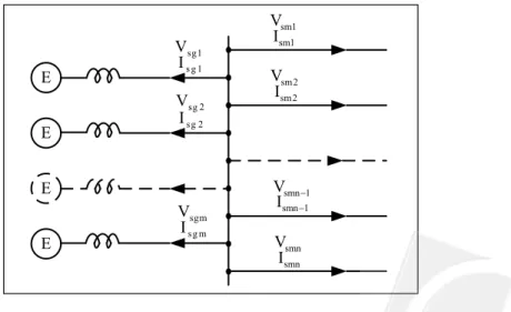
Figure 1 shows a simple one-node small power system which contains m generators and n loads. According to Kirchhoff’s current law (KCL), the current relationship between supplying and receiving elements can be expressed as

1 1 0 m n sgk sml k l I I = = + =

∑

₍₂₎

Any one of the currents can be represented by the combination of the others. Similarly, according to the Kirchhoff’s voltage law (KVL), the terminal voltages of all the components connected to the same node are identical. The relationship can be expressed as

1 2 ... 1 2 ...

sg sg sg m sm sm sm n

V =V = =V =V =V = =V ₍₃₎

3. ARRANGEMENT OF MATHEMATICAL MODELS

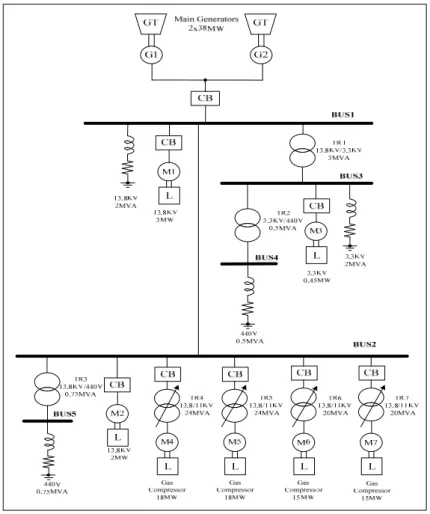
3.1 System Configuration

Figure 2 shows the configuration of an offshore gas-turbine power system that includes gas-turbine prime movers, synchronous generators and excitation systems, three-phase power transformers, induction motors, protection and measuring equipment, and lumped static loads[20]. E E E E s g 1 Isg1 V sg 2 V sgm V sm1 V sm2 V smn 1 V ₋ smn V sg 2 I sg m I sm1 I sm2 I smn 1 I ₋ smn I

(4)

Figure 2 Configuration of an offshore gas-turbine power system

3.2 Gas-Turbine Prime Mover

The single-shaft gas turbine model mainly consists of two parts, namely the single-shaft gas turbine and its control associated with fuel system[21]. The control system includes four important functions: speed control, temperature control, acceleration control, and upper and lower fuel limits. Speed control mechanism is suitable for either droop or isochronous control and operates satisfactorily within certain speed ranges. The temperature control is the normal mechanical mechanism for limiting gas turbine output at a predetermined firing temperature, either independent of or dependent on the variation in ambient temperature or fuel characteristics. The acceleration control is used primarily during gas turbine start-up to limit the rate of rotor acceleration prior to reaching the set governor speed and provides a secondary function during normal operation to reduce fuel flow. The fuel system outputs a volume of fuel which is proportional to the fuel intake for the turbine.

It is often sufficient to consider a simplified model in which the temperature control and minor characteristics of the gas turbine are limited. This model, shown in schematic form in Figure 3, may be represented by the following equations together with the information given in the figure.

(5)

1 1 1 1 1 2 4 2 2 2 2 IL 2 2 2 2 3 3 3 3 3 1 K 0 0 0 0 T T X X K K ( 1 F )K K 1 p X 0 X 0 P T T T T X X F K 1 0 0 0 0 T T Δω ⎡− ⎤ ⎡ ⎤ ⎢ ⎥ _⎢ _⎥ ⎢ ⎥ _⎢ _⎥ ⎡ ⎤ _⎢ _⎥⎡ ⎤ ⎡ ⎤ − − − ⎢ ⎥ ⎢ ⎥₌_⎢ _⎥⎢ ⎥₊ ⎢ ⎥ ⎢ ⎥ ⎢ ⎥ _⎢ _⎥⎢ ⎥ ⎢ ⎥ ⎢ ⎥ ⎢ ⎥ ⎢ ⎥ ⎢ ⎥ ⎣ ⎦ _⎢ ₋ _⎥⎣ ⎦ _⎢ _⎥⎣ ⎦ ⎢ ⎥ _⎢ _⎥ ⎢ ⎥ ⎣ ⎦ ⎣ ⎦ ₍₄₎ 1 1 K 1 sT+ 4 K 2 f 3 3 K 1 sT+ 2 2 K 1 sT+ Δω X1 P1L X2 X3 F2 W r ω 2 F2 r f =1.3(W −0.23) 0.5(1+ − ω)

Figure 3 Schematic diagram of simplified single-shaft gas turbine

3.3 Synchronous Machine

When synchronous generators supply isolated loads as, for example, in marine and offshore power systems, the buses to which the generators are connected cannot be treated as infinite. As a consequence the bus voltage will fluctuate at the instant of load change. A typical example is the sequential switching of group induction motors.

A three-phase salient-pole synchronous generator has three symmetrical windings on the stator, an excitation, and two damper windings on the rotor. In general, the mutual inductance between any two windings on the d-axis has the same amplitude Lmd; the mutual inductance between any two windings on the q-axis has the same amplitude Lmq. In the two-axis rotor reference frame, the voltage equations for the synchronous machine can be expressed as

qs s q r d mq r md r md qs ds r q s d r mq md md ds kq mq kq kq kq fd md fd fd md fd kd md md kd kd kd v r pL L pL L L i v L r pL L pL pL i v pL 0 r pL 0 0 i v 0 pL 0 r pL pL i v 0 pL 0 pL r pL i ω ω ω ω ω − − − ⎡ ⎤ ⎡ ⎤ ⎡ ⎤ ⎢ ⎥ ⎢ _{− −} ₋ ⎥ ⎢ ⎥ ⎢ ⎥ ⎢ ⎥ ⎢ ⎥ ⎢ ⎥ ⎢= − + ⎥ ⎢ ⎥ ⎢ ⎥ ⎢ ₋ ₊ ⎥ ⎢ ⎥ ⎢ ⎥ ⎢ ⎥ ⎢ ⎥ ⎢ ⎥ ⎢ ₋ ₊ ⎥ ⎢ ⎥ ⎣ ⎦ ⎣ ⎦ ⎣ ⎦₍₅₎

where vds and ids are d-axis stator voltage and current, vqs and iqs are q-axis stator voltage and current, vkq, and ikq are q-axis rotor damper winding voltage and current, vfd, vkd, ifd, and ikd are excitation voltage, d-axis damper winding voltage, excitation current, and d-axis damping winding current, rs, rfd, rkd, and rkq are stator resistance, excitation winding resistance, d-axis

(6)

damper winding resistance, and rotor q-axis damper winding resistance, Ld, Lq, Lfd, Lkd, and Lkq are d-axis inductance, q-axis inductance, excitation winding inductance, d-axis damper winding inductance, q-axis damper winding inductance, Lmd and Lmq are d-axis mutual inductance and q-axis mutual inductance, and p is the differential operand[22].

3.4 Excitation System

Almost all synchronous generators in the industrial power system operate with automatic voltage regulators (AVRs) to control generator terminal voltage. As soon as a deviation in terminal voltage is detected, the AVR should be responsive and regulate the excitation voltage to control the terminal voltage of the synchronous generator within preset limits.

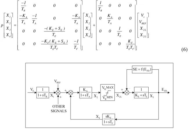
Two types of AVRs applied widely to the industry have been recommended by IEEE study committees and are designated “type 1” and “type 2” models[23-26]. Figure 4 shows the block diagram of type 1 AVR model. The state space equation for the model can be expressed as

R R 1 A A 1 A s A A A A 2 2 REF 3 E E 3 2 L E E 4 4 2 L F F E E E F E F F 1 1 0 0 0 0 0 0 T T X K 1 K X K V 0 0 0 0 T T T T X X V p X ( K S ) X 1 X 0 0 0 0 0 0 T T X X X K K ( K S ) 1 0 0 0 0 0 T T T T T − ⎡ ⎤ ⎡ ⎤ ⎢ ⎥ ⎢ ⎥ ⎢ ⎥ ⎢ ⎥ ⎡ ⎤ ⎢− − − ⎥⎡ ⎤ ⎢ ⎥⎡ ⎢ ⎥ ⎢ ⎥⎢ ⎥ ⎢ ⎥⎢ ⎢ ⎥₌⎢ ⎥⎢ ⎥₊⎢ ⎥⎢ ⎢ ⎥ ⎢ − + ⎥⎢ ⎥ ⎢ ⎥⎢ ⎢ ⎥ ⎢ ⎥⎢ ⎥ ⎢ ⎥⎢ ⎢ ⎥ ⎢ ⎥ ⎣ ⎣ ⎦ ⎢ ⎥⎣ ⎦ ⎢ ⎥ ⎢ − + − ⎥ ⎢ ⎥ ⎢ ⎥ ⎢_⎢ ⎥_⎥ ⎢ ⎥ _⎣ _⎦ ⎣ ⎦ ⎤ ⎥ ⎥ ⎥ ⎥ ⎢ _⎥⎦ (6) A A K 1 sT+ R 1 1 sT+ X₁ X2L X3 R V R V 2 X E E 1 K +sT FD SE f (E )= FD E 4 X F F sK 1 sT+ S V REF V

Figure 4 Block diagram of IEEE type 1 AVR model

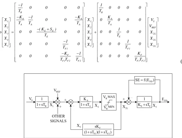
Figure 5 shows the block diagram of type 2 AVR model. The state space equation for the model can be expressed as

(7)

R R A A A 1 1 A A A A 2 2 E E 3 3 E E 4 4 5 5 F 1 F 1 F F F 1 F 2 F 2 F 1 F 2 1 1 0 0 0 0 0 0 0 0 T T K 1 K K 0 0 0 0 0 0 X X T T T T X X ( K S ) 1 0 0 0 0 0 0 0 0 p X X T T X X 1 1 0 0 0 0 0 0 0 0 X X T T K 1 K 0 0 0 0 0 0 0 T T T T T − ⎡ ⎤ ⎡ ⎢ ⎥ ⎢ ⎢ ⎥ ⎢ − − − ⎢ ⎥ ⎢ ⎡ ⎤ _⎢ _⎥⎡ ⎤ _⎢ ⎢ ⎥ _⎢ _⎥⎢ ⎥ _⎢ ⎢ ⎥ _⎢ ₋ ₊ _⎥⎢ ⎥ ⎢ ⎥=⎢ ⎥⎢ ⎥+ ⎢ ⎥ _⎢ _⎥⎢ ⎥ ⎢ ⎥ _⎢ ₋ _⎥⎢ ⎥ ⎢ ⎥ _⎢ _⎥⎢ ⎥ ⎣ ⎦ ⎣ ⎦ ⎢ ⎥ ⎢ − − ⎥ ⎢ ⎥ ⎢ ⎥ ⎣ ⎦ ⎣ S REF 2 L 2 L 2 L V V X X X ⎤ ⎥ ⎥ ⎥ ⎡ ⎤ ⎥ ⎢ ⎥ ⎥ ⎢ ⎥ ⎢ ⎥ ⎢ ⎥ ⎢ ⎥ ⎢ ⎥ ⎢ ⎥ ⎢ ⎥ ⎢ ⎥ ⎢ ⎥ ⎢ _{⎥ ⎣} _⎦ ⎢ ⎥ ⎢ ⎥ ⎢ ⎥ ⎢ _⎥⎦ ₍₇₎ A A K 1 sT+ R 1 1 sT+ X₁ 2L X X3 R V R V 2 X E E 1 K +sT FD SE f (E )= FD E 5 X F F1 F2 sK (1 sT )(1 sT )+ + S V REF V

Figure 5 Block diagram of IEEE type 2 AVR model

In the models the field voltage provides connection to the synchronous generator equations. In other words, the output of the AVR is an input to the generator and the output (terminal voltage) of the generator represents an input to AVR.

3.5 Induction Machine

A three-phase induction machine has three symmetrical windings on the stator and squirrel-cage shaped conductors or symmetrical windings on the rotor. With all electrical variables and parameters of the machine referred to the stator, the voltage equation for the induction machine in the two-axis stationary reference frame can be expressed as

qs s ss m qs ds s ss m ds qr m r m r rr r rr qr dr r m m r rr r rr dr v r pL 0 pL 0 i v 0 r pL 0 pL i v pL L r pL L i v L pL L r pL i ω ω ω ω + ⎡ ⎤ ⎡ ⎤ ⎡ ⎤ ⎢ ⎥ ⎢ ₊ ⎥ ⎢ ⎥ ⎢ ⎥ ⎢₌ ⎥ ⎢ ⎥ ⎢ ⎥ ⎢ − + − ⎥ ⎢ ⎥ ⎢ ⎥ ⎢ ₊ ⎥ ⎢ ⎥ ⎢ ⎥ ⎢ ⎥ ⎢ ⎥ ⎣ ⎦ ⎣ ⎦ ⎣ ⎦₍₈₎

where vds and ids are d-axis stator voltage and current, vqs and iqs are q-axis stator voltage and current, vdr and idr are d-axis rotor voltage and current, vqr and iqr are q-axis rotor voltage and current, rs and rr are stator resistance and rotor resistance, Lss and Lrr are stator inductance and rotor inductance, Lm is the magnetizing inductance, and p is the differential operand[22].

(8)

3.6 Mechanical Model

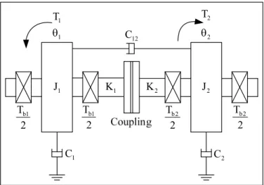
Figure 6 gives the schematic representation of a simple two-mass system. As the system is represented by second-order differential equations in θ1 and θ2, the system will have the undamped natural frequency given by fn=(π/2)(K/J1+K/J2)1/2 which is sufficiently accurate for most applications[27]. The shaft torque may be considered less than the air-gap torque under transient conditions. During the initial starting period the air-gap torque pulsates at twice slip frequency. If any of these frequencies coincides with the natural frequency of the system, resonance can occur. This may lead to torque amplification and possible failure of the coupling or shaft.

This model may be represented by the following equations together with the information given in the figure.

1 1 1 12 12 1 1 1 1 1 1 1 b1 1 1 2 2 2 b2 2 12 2 12 2 2 2 2 2 2 2 0 1 0 0 0 0 0 0 T C C C K K 1 1 0 0 J J J J J J T p T 0 0 0 1 0 0 0 0 T C C C 1 1 K K 0 0 J J J J J J θ θ ω ω θ θ ω ω ⎡ ⎤ ⎡ ⎤ ⎢ ⎥ ⎢ _{⎥ ⎡ ⎤} ⎡ ⎤ _⎢− − − _⎥⎡ ⎤ _⎢ − ⎥ ⎢ ⎥ ⎢ ⎥ _⎢ _⎥⎢ ⎥ _⎢ ⎥ ⎢ ⎥ ⎢ ⎥₌_⎢ _⎥⎢ ⎥₊_⎢ ⎥ ⎢ ⎥ ⎢ ⎥ _⎢ _⎥⎢ ⎥ _⎢ ⎥ ⎢ ⎥ ⎢ ⎥ _⎢ ₋ ₋ ₋ _⎥⎢ ⎥ _⎢ ₋ ₋ _⎥ ⎢ ⎥ ⎢ ⎥ ⎢ ⎥ ⎣ ⎦ _⎢ _⎥⎣ ⎦ _⎢ _⎥⎣ ⎦ ⎢ ⎥ ⎢ ⎥ _⎣ _⎦ ⎣ ⎦ ₍₉₎

In the equations, J1 and J2 are the inertias of rotating mass 1 including coupling and mass 2, K1 and K2 are shaft stiffness, C1, C2, and C12 are self and mutual damping coefficients, Tb1 and Tb2 are bearing loss torques, and K is the sum of K1 and K2.

1 θ θ₂ 1 T T2 1 J K₁ K₂ J₂ 1 C C₂ b1 T 2 b1 T 2 b2 T 2 b2 T 2 12 C

Figure 6 The schematic representation of a simple two-mass system

3.7 Three-Phase Power Transformer

The components of the power system concerned with system interconnection include transmission lines, power transformers, and auto-transformers. In the standalone power systems where the actual physical distances are negligible, the transmission lines are considered to

(9)

possess low impedances, and the connection between generators on induction motors are facilitated by including resistance and reactance of the transmission lines into the machine models.

The voltage equations for the power transformer and auto-transformer can be expressed as

q1 1 11 m q1 d 1 1 11 m d 1 q 2 m 2 22 q 2 d 2 m 2 22 d 2 v r pL 0 pL 0 i v 0 r pL 0 pL i v pL 0 r pL 0 i v 0 pL 0 r pL i + ⎡ ⎤ ⎡ ⎤ ⎡ ⎤ ⎢ ⎥ ⎢ ₊ ⎥ ⎢ ⎥ ⎢ ⎥ ⎢₌ ⎥ ⎢ ⎥ ⎢ ⎥ ⎢ + ⎥ ⎢ ⎥ ⎢ ⎥ ⎢ ₊ ⎥ ⎢ ⎥ ⎢ ⎥ ⎢ ⎥ ⎢ ⎥ ⎣ ⎦ ⎣ ⎦ ⎣ ⎦₍₁₀₎

where vd1 and id1 are d-axis primary voltage and current, vq1 and iq1 are q-axis primary voltage and current, vd2 and id2 are d-axis secondary voltage and current, vq2 and iq2 are q-axis secondary voltage and current, r1 and r2 are primary resistance and secondary resistance, L11 and L22 are primary and secondary inductance inductance, Lm is magnetizing inductance, and p is the differential operand.

3.8 Static Load

The lumped static load can be modeled as a resistance load and a reactive load. The voltage equations for the load can be expressed by

0 0 qk sk sk qk dk sk sk dk v r pL i v r pL i + ⎡ ⎤ ⎡₌ ⎤ ⎡ ⎤ ⎢ ⎥ ⎢ ₊ ⎥ ⎢ ⎥ ⎣ ⎦ ⎣ ⎦ ⎣ ⎦₍₁₁₎

where vdk and idk are d-axis voltage and current, vqk and iqk are q-axis voltage and current, rsk and Lsk are resistance load and reactive load, and p is the differential operand.

4. PRACTICAL APPLICATION OF ANALYSIS

To illustrate the use of the theoretical techniques and methods of solution discussed in previous sections, a practical example has been chosen to demonstrate the range of application of the simulation models presented.

4.1 SimPowerSystems Models

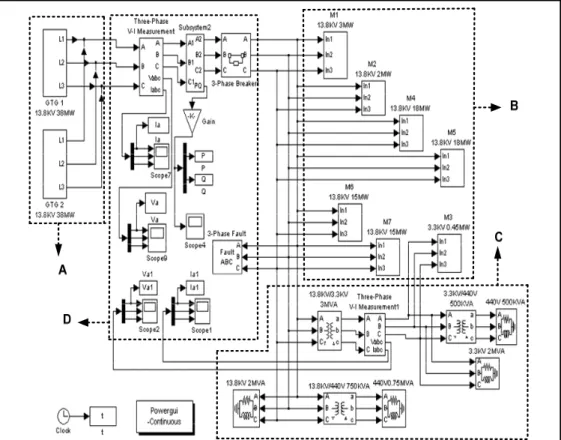
The purpose of the simulation is to study the dynamic performance of an offshore power system when subjected to motor starting sequentially and fault condition. To illustrate the versatility of the analysis, two studies were conducted on the offshore power system shown in Figure 2. Figure 7 shows the SimPowerSystems model for the system. The configuration mainly includes four parts: models for the generation systems (section A), models for the induction machines (section B), models for power transformers and static loads (section C), and models for measurement devices (section D). The principal data for the study are given in Appendix.

(10)

Figure 7 The configuration of PSB model for the system depicted in Figure 2

4.2 Simulation Sequences

1. Normal Operation: Motor Starting Sequentially

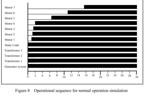
Generators were connected to bus 1, and then seven motors were switched on to the supply in sequence as outlined in Figure 8. The total simulation time was 30 seconds.

2. Abnormal Operation: Three-Phase Balanced Fault Occurred at the Generator Bus Generators were connected to bus 1, and then seven motors were switched on to the supply in sequence as outlined in Figure 9. A three-phase balanced fault occurred at the generator bus at 23.0 second and cleared at 23.3 second. The total simulation time was 30 seconds.

4.3 Simulation Results and Comments

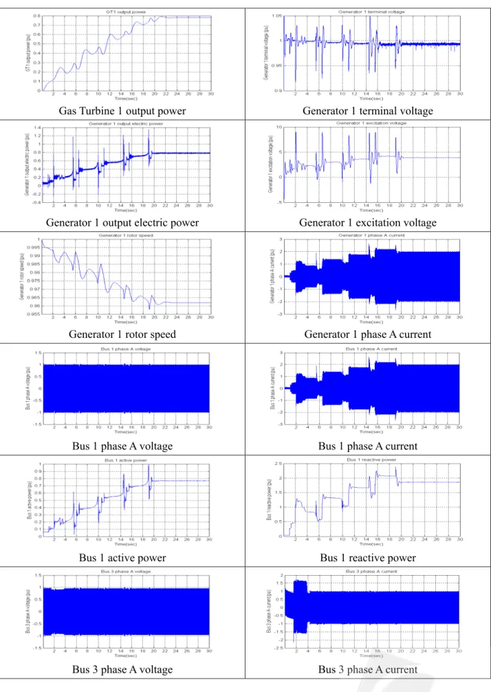
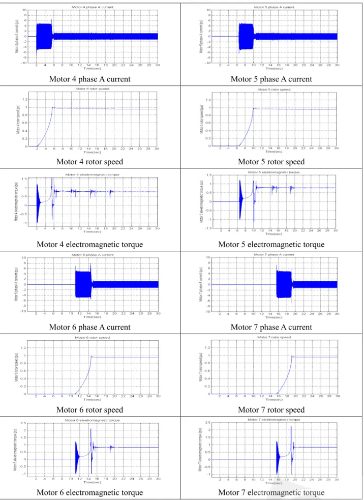
The simulation results of normal operation, referred to the ratings of components, are shown in Figure 10. In the study, seven motors were switched on to the supply in sequence. This caused voltage reductions coinciding with individual motor starting. After short time delays, voltages began to recover due to exciter and speed governor action. In other words, on every occasion that a motor was switched on to the supply a fluctuation of bus voltage and frequency was imposed on the system. Finally, steady-state operation was reached.

The simulation results of abnormal operation, referred to the ratings of components, are shown in Figure 11. In the study, motors were switched on to the supply in sequence. After all motors had run-up successfully a three-phase balanced fault was applied after 23.0 second at the

(11)

generator bus. The system response subsequent to the application of the fault was characterized by an average voltage reduction at the bus of approximately 100 percent. The system frequency increased by a small amount due to the sudden loss of active power. In addition, low voltages recorded at other buses led to reduction in speed of operation for the remaining induction motors. After fault clearance, at 23.3 second, the generator terminal voltages recovered and the post-fault recovery of the induction motors was rapidly reestablished.

Simulation results show that the system operated satisfactorily under those conditions. At the preliminary planning stage for this scheme it was considered that the fault clearance time used should be such that all possible inaccuracies associated with protection operation would be fully covered. An overall clearance time of 300ms was therefore selected.

Figure 8 Operational sequence for normal operation simulation

(12)

Gas Turbine 1 output power Generator 1 terminal voltage

Generator 1 output electric power Generator 1 excitation voltage

Generator 1 rotor speed Generator 1 phase A current

Bus 1 phase A voltage Bus 1 phase A current

Bus 1 active power Bus 1 reactive power

(13)

Motor 4 phase A current Motor 5 phase A current

Motor 4 rotor speed Motor 5 rotor speed

Motor 4 electromagnetic torque Motor 5 electromagnetic torque

(14)

Gas Turbine 1 output power Generator 1 terminal voltage

Generator 1 output electric power Generator 1 excitation voltage

Generator 1 rotor speed Generator 1 phase A current

Bus 1 active power Bus 1 reactive power

(15)

(16)

5. CONCLUSIONS

This research investigated the dynamic performance of an offshore gas-turbine power system operating in normal and abnormal situations. A method for predicting dynamic responses of interconnected machine systems was introduced and employed to connect system components. The mathematical models for the system components, including gas-turbine model, electric machine model, electromechanical model, and three-phase power transformer model, were developed to cater for the dynamic behavior of the system using Simulink and SimPowerSystems. Simulation results show that the system operated satisfactorily under those conditions. This type of study is important in system planning to design required system enhancements, in system operations to establish secure operating limits, and for designing appropriate remedial control and protection schemes to improve the power system response to disturbances.

REFERENCES

[1] Hung, W. W., “Dynamic simulation of gas-turbine generating unit,” IEE Proceedings C-- Generation, Transmission and Distribution, Vol. 138, Issue 4, 1991, pp. 342–350

[2] Doughty, R. L., L. Gise, E. W. Kalkstein, and R. D Willoughby, “Electrical studies for an industrial gas turbine cogeneration facility,” IEEE Transactions on Industry Applications, Vol. 25, Issue 4, 1989, pp. 750-765

[3] Bagnasco, A., B. Delfino, G. B. Denegri, and S. Massucco, “Management and dynamic performances of combined cycle power plants during parallel and islanding operation,” IEEE Transactions on Energy Conversion, Vol. 13, Issue 2, 1998, pp. 194–201

[4] Hajagos, L. M. and G. R. Berube, “Utility experience with gas turbine testing and modeling,” IEEE Power Engineering Society Winter Meeting, Vol. 2, 2001, pp. 671-677

[5] N. Chiras, C. Evans, and D. Rees, “Nonlinear gas turbine modeling using NARMAX structures,” IEEE Transactions on Instrumentation and Measurement, Vol. 50, Issue 4, Aug. 2001, pp. 893-898

[6] Nagpal, M., A. Moshref, G. K. Morison, and P. Kundur, “Experience with testing and modeling of gas turbines,” IEEE Power Engineering Society Winter Meeting, Vol. 2, 2001, pp. 652-656 [7] Jurado, F. and J. R. Saenz, “Adaptive control of a fuel cell-microturbine hybrid power plant,”

IEEE Power Engineering Society Summer Meeting, Vol. 1, 2002, pp.76-81

[8] G. Steinfeld, H. C. Maru, and R. A. Sanderson, “High efficiency carbonate fuel cell/turbine hybrid power cycle,” IEEE Energy Conversion Engineering Conference, Vol. 2, Aug. 1996, pp. 1123-1127

[9] Hamilton, S., “Fuel cell-mtg hybrid: the most exciting innovation in power in the next 10 years,” IEEE Power Engineering Society Summer Meeting, Vol. 1, 1999, pp. 581-586

[10] Berta, G. L., F. Durelli, and A. P. Prato, “A special arrangement of hybrid gas turbines,” IEEE Energy Conversion Engineering Conference, Vol. 5, 1990, pp. 495-501

(17)

IEEE Transactions on Power Systems, Vol. 18, Issue 3, 2003, pp. 1110-1115

[12] Rowen, W. I., “Dynamic response characteristics of heavy duty gas turbines and combined cycle systems in frequency regulating duty,” IEEE Colloquium on Frequency Control Capability of Generating Plant, 1995, pp. 6/1-6/6

[13] Kunitomi, K. A., Kurita, Y. Tada, S. Ihara, W. W. Price, L. M. Richardson, and G. Smith, “Modeling combined-cycle power plant for simulation of frequency excursions,” IEEE Transactions on Power Systems, Vol. 18, Issue 2, 2003, pp. 724-729

[14] Kakimoto, N. and K. Baba, “Performance of gas turbine-based plants during frequency drops,” IEEE Transactions on Power Systems, Vol. 18, Issue 3, 2003, pp. 1110-1115

[15] Jong-Wook Kim and Sang Woo Kim, “Design of incremental fuzzy PI controllers for a gas-turbine plant,” IEEE/ASME Transactions on Mechatronics, Vol. 8, Issue 3, 2003, pp. 410-414

[16] Akins, B. and R. G. Harley, The General Theory of Alternating Current Machines, Chapman and hall, 1975

[17] Smith, J. R. and M.-J. Chen, Three-Phase Electrical Machine Systems, Research Studies Press Ltd., 1993

[18] Tsao, T., S. Chen, C. Huang and W. Lin, “Dynamic response analysis of marine power systems,” IEEE Proceedings C-- Generation, Transmission and Distribution, Vol. 135, 1988, pp. 74-78

[19] Smith, J. R. and M.-J. Chen, Three-Phase Electrical Machine Systems, Research Studies Press Ltd., 1993.

[20] Stewart, I. D., “Offshore power generation-limited life expectancy,” International Conference on Opportunities and Advances in International Electric Power Generation, 1996, pp. 25-28 [21] Rowen, W. I., “Simplified mathematical representations of heavy-duty gas turbine,” ASME

Journal of Engineering for Power, 83-GT-63

[22] Krause, P. C., Analysis of Electric Machinery and Drive System, 2nd Ed., McGRAW-Hill Book Co., 2001

[23] IEEE Guide for Identification, Testing and Evaluation of the Dynamic Performance of Excitation Control Systems, ANSI/IEEE Std 421A-1978, June 1978

[24] IEEE Committee Report, “Excitation system models for power system stability studies,” IEEE Transaction on Power Apparatus and Systems, PAS-100, 1981, pp. 494-509

[25] IEEE Recommended Practice for Excitation System Models for Power System Stability Studies, IEEE Std 421.5-1992, 1992

[26] IEEE Committee Report, “Computer models for representation of digital-based excitation systems,” IEEE Transaction on Energy Conversion, Vol. 10, Issue 4, Dec. 1996, pp. 706-713 [27] Smith, J. R., A. F. Stronach, and T. Tsao, “Digital simulation of marine electromechanical