半導體供應鏈生產整合模式資源分配模式之研究
蔣明晃 台大工商管理系副教授 摘要:本研究中運用分解法對一個供應鏈生產規劃 與排程模型進行運算,將原有的大型混合性整數規劃模 型分解為一個主模型與數個子模型。該分解模型可根據 產能、物料、以及需求的限制,進行總成本的最小化, 並產生明顯可行而良好的生產排程。分解法會反覆進行 運算,直到與最佳值之差異小於 0.05 時方才停止,並 產生出最終的解。本研究更以模擬方式,比較經驗法 則、整體規劃模型、以及分解規劃模型三種規劃方式, 在四十八種不同情境下的績效,並加以比較。研究結果 中,分解規劃模型可以提供近乎最佳的績效,一般的經 驗法則反而無法維持規劃績效的穩定。儘管與經驗法則 和整體規劃模型相比,分解規劃模型在簡單的情境中運 算耗時較久﹔隨著情境越趨複雜,後者的運算績效卻會 逐漸超越前兩者。因此,在實務運用上,分解規劃模型 顯然是較理想的生產規劃排程工具。Abstract – This paper focuses on developing a
decomposition model to efficiently solve multiplant production planning and scheduling problems. Two other conventional approaches, business rules and monolithic model, are also under investigation for the comparison purposes. All three approaches needed to complete two tasks for a multiplant production planning and scheduling problem, namely, assign orders to plants and generate feasible production schedules. The results of the three approaches simulated under 48 scenarios were collected and compared. From the comparison results, this paper concluded that the decomposition model would be a better production planning and scheduling tool in practice.
INTRODUCTION
As manufacturers are no longer effectively compete in isolation of their suppliers and other entities in the supply chain, how to efficiently solve a multiplant production planning and scheduling problem within the chain is crucial for a manufacturer to maintain its competitiveness. Using monolithic approach as a modeling tool to solve multiplant production planning and scheduling problems often encounters numerous computation difficulties. Consequently, many enterprises continue their traditional practice, using business rules to manage their production planning and scheduling problems. However, it is implemented at the expense of not practicing integrated planning. To overcome the computation difficulties and to obtain an integrated production planning and scheduling
solution, a new technique is proposed by Shapiro [1] known as decomposition approach.
Conventionally, the monolithic approach formulates the production planning and scheduling problem as a large mixed-integer linear programming problem, which can obtain an optimal solution, but at the expense of long computation time. On the other hand, the business rules allows the production planners to obtain a feasible production planning within a short period of time, but the practice does not consider issues like material, cost, inventory, capacity and demand simultaneously in an integrated point of view. As both approaches are not satisfactory, the decomposition approach has become an attractive alternative.
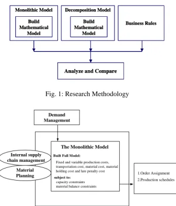
The decomposition technique has been proposed for years by Dzielinski and Gomory [2]. Dzielinski and Gomory [2] originally applied Dantzig-Wolf decomposition principle to solve lot size, inventory and allocation problem. It is only until recently, Shapiro [1] further extended the concept to the production planning and scheduling problems with the addition of a feedback intelligent, the shadow prices, to reflect the cost penalty of the constrained resources. This paper aims to implement a multiplant production planning and scheduling problem using the decomposition technique and compare the strength and weakness of the three approaches, business rules, monolithic model, and decomposition model. All three approaches are used to complete two major tasks in a multiplant production planning and scheduling problem, namely, assign orders to plants and generate feasible production schedules. From Fig. 1, both the monolithic model and the decomposition model adopted mixed integer programming (mathematic model) to assign orders to plants and generate feasible schedules. While on the contrary, the business rules assign orders to plants according to four business rules, taking turns, product types, average capacity and due date. Once the orders are assigned to each plant, each plant can generate a production schedule.
In the following sections, three multiplant production planning and scheduling models are introduced. Then the three models are tested under 48 scenarios for comparison purpose.
Before introducing the decomposition approach, a brief overview of the monolithic model is presented firstly. The monolithic model considered all the influential constraints and the objectives function as a whole simultaneously as presented in Fig. 2. The outputs of the model are order assignments and production schedules. The detail of objective function and constrains are shown as following:
Objective Function:
Fixed production cost +Variable production cost +Late penalty cost +Material cost +Material holding cost
Constraints:
Demand-Production Constraints
One Order Only Produced by Single Plant Capacity Constraints
Material Inventory Balance Constraints Materials Purchasing Constraints General non-negativity Constraints
BUSINESS RULES
Usually, these business rules are firstly used to assign orders to plants, and then follow by the production planning and material requirement planning. In this paper, there are two ways to utilize the results of these business rules. Firstly, the results are used in comparison with the monolithic model and the decomposition model. Secondly, the result of the business rules also served as initial solutions to the decomposition model in the iteration procedures as shown in Fig. 4. These business rules are stated below:
1. Taking Turns Rules
After order received, they are assigned to plant alternately. Then, each plant independently plans its own production schedule and material acquisition.
2. Average Capacity
Manually assign orders to plants in order to make all plants have nearly equal production loading. Then, each plant independently plans its own production schedule and material acquisition.
3. Product Type
Using product type to assign the orders to the plants, for example product type A will be assigned to plant 2. Then, each independently plant plans its own production schedule and material acquisition.
4. Due Date
Sort the orders according to their due date, then assign order to plants sequentially to eliminate the possibility of orders with the closed due date are produced by the same plant. Then, each plant
plans its own production schedule and material acquisition.
DECOMPOSITION MODEL
The construction of the decomposition model is much complicated than the monolithic model. The decomposition model as shown in Fig. 3, breaks down a large-scale mixed-integer production planning problem into a master model and several smaller submodels.
Each submodel minimizes total plant production costs and generates a demonstrably good plant production schedule subject to materials, capacity and demand constraints as listed below:
Objective Function:
Fixed production cost + Variable production cost + Late penalty cost + Material cost + Material holding cost +Shadow price cost
Constraints (Single Plant Only): Demand-Production Constraints
One Order Only Produced by Single Plant Capacity Constraints
Material Inventory Balance Constraints Materials Purchasing Constraints General Constraints
These information can be fed into the master model as additional inputs to the initial results obtained from heuristics. The master model then minimizes the total avoidable costs subject to resource constraints and weight constraints as presented below to provide either feedback information (shadow prices) or a global production plan.
Objective Function:
Minimize the total avoidable production cost ($)
Resource Constraints:
Make sure production will meet the demand under restriction of plant capacities.
Weight Constraints:
♦ Ensure only one feasible production plan is selected for each order.
♦ Ensure one order only produced by a single plant. The final solution of the decomposition model is found by an iterative procedure as indicated in Fig 4, which stops when the optimality gap is smaller than 0.5%.
SIMULATIONS AND COMPARISONS
In this paper, simulations were run for the business rules, the monolithic model and the decomposition model. These
simulations used a software package, ILOG to test 12 scenarios that built in different business conditions, such as price rising and price falling (refer to Table 1) on different production capabilities and plant capacities which sums up to 48 scenarios as indicated in Figure 5.
The 48 combinations can be distributed into four cases according production capability and the plant capacity, they are,
1. Small scale, loose capacity: two plants available for production, the planning horizon is 10 weeks, and average demand per week is much less than weekly capacity in a plant.
2. Small scale, tight capacity: two plants available for production, the planning horizon is 10 weeks, and average demand per week is close to weekly capacity in a plant.
3. Large scale, loose capacity: three plants available for production, the planning horizon is 13 weeks, and average demand per week is much less than weekly capacity in a plant.
4. Large scale, tight capacity: three plants available for production, the planning horizon is 13 weeks, and average demand per week is close to weekly capacity in a plant.
Each case above will test for the twelve production scenarios as listed in Table 1.
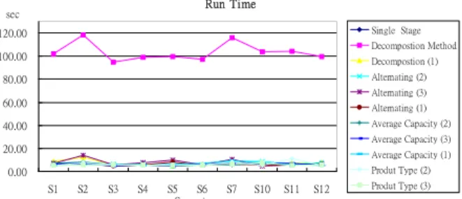
The results of three approaches simulated under 48 scenarios are collected and compared. From Fig. 6 and 8, the decomposition model can generate a solution very close to the optimal whereas the business rules cannot guarantee a stable performance. Even though the simulation time required for the decomposition model in solving a simple production problem is not short enough to compete with the business rules or the monolithic model as shown in Fig 7, however, as the production problems gets complicated, the decomposition model will outperform the business rules and the monolithic model as illustrated in Fig 9.
CONCLUSIONS
From the comparison analysis of the simulation results, following conclusions are obtained:
The incapability of the business rules
The business rules used in this thesis, such as taking turns, product type and average capacity may generate a schedule quickly, but the schedule is not guaranteed to be a reliable and cost-efficient one. Furthermore, the company does not integrate all production functions such as material procurement and inventory control to support the production. As the concepts of SCM and APS become prevailing in today’s global market competition, using business rules may likely to cause a company to lose its
competitiveness to high production cost and ineffective internal coordination.
The computation difficulty of the monolithic model
The monolithic model always produces out an optimal solution, however, at the cost of requiring long computation time. The complexity of the mathematical programming in the monolithic model by using numerous zero-one variables has prevented the model to be implemented in today’s computing technology. Thus, the model is not recommended for the practical implementation.
The decomposition model can generate a demonstrably good production schedule in a reasonable time.
Even though the simulation time required in solving a simple production problem is not short enough to compete with the business rules or the monolithic model, however, as the production problems gets complicated, the decomposition model will outperform the business rules and the monolithic model. If the decomposition model can be coordinated with other functions in APS, such as Demand Planning (DP) and Factory Planning (FP), the decomposition approach can be introduced to business in real practice.
TABLES AND FIGURES
Monolithic Model Decomposition Model
Build Mathematical
Model
Analyze and Compar e
Business Rules Build
Mathematical Model
Monolithic Model Decomposition Model
Build Mathematical
Model
Analyze and Compar e
Business Rules Build
Mathematical Model
Fig. 1: Research Methodology
Mater ial Planning Inter nal supply chain management
Demand Management
1.Order Assignment 2.Production schedules The Monolithic Model
Built Full Model:
Fixed and variable production costs, transportation cost, material cost, material holding cost and late penalty cost subject to:
capacity constraints material balance constraints
Pr oduction Submodel Plant 1 Pr oduction Submodel Plant N … Objective Function: Minimization … Pr oduction Utilization Plant 1 Avoidable Costs Pr oduction Utilization Plant N Avoidable Costs … Weights Weights ... New Feasible Schedule + Avoidable Costs New Feasible Schedule + Avoidable Costs Shadow Prices Shadow Prices
Global Constr aints: ≥ Demand
= . . . = 1 . . . 1 Submodel Pr oduction Submodel Plant 1 Pr oduction Submodel Plant N … Objective Function: Minimization … Pr oduction Utilization Plant 1 Avoidable Costs Pr oduction Utilization Plant N Avoidable Costs Pr oduction Utilization Plant 1 Avoidable Costs Pr oduction Utilization Plant 1 Avoidable Costs Pr oduction Utilization Plant N Avoidable Costs Pr oduction Utilization Plant N Avoidable Costs … Weights Weights ... New Feasible Schedule + Avoidable Costs New Feasible Schedule + Avoidable Costs Shadow Prices Shadow Prices
Global Constr aints: ≥ Demand
= . . . = 1 . . . 1
Global Constr aints: ≥ Demand
= . . . = 1 . . . 1 ≥ Demand = . . . = 1 . . . 1 Demand = . . . = 1 . . . 1 Submodel
Fig. 3: Decomposition Model
Data Apply Heuristics Feasible Schedule Feasible Schedule Optimize LP Model Create More Schedules Incumbent Demonstrably Good? Return to Lagrangean Submodel? Incumbent Scheduling Solution Optimize IP Model Optimize Lagrangean Submodel Yes No Yes No Yes Terminate with Incumbent Solution Iter ation Pr ocedur es
Shadow Prices No Optimality gap ≤ 0.05 Data Apply Heuristics Feasible Schedule Feasible Schedule Optimize LP Model Create More Schedules Incumbent Demonstrably Good? Return to Lagrangean Submodel? Incumbent Scheduling Solution Optimize IP Model Optimize Lagrangean Submodel Yes No Yes No Yes Terminate with Incumbent Solution Iter ation Pr ocedur es
Shadow Prices
No
Optimality gap ≤ 0.05
Fig 4: Iteration Procedure of Decomposition
Models
Per for mance Measur es Monolithic Model Business Rules Decomposition Model Scenar ios Pr oduction Capability •Lar ge Scale •Small Scale Plant Capacity •Loose •Tight Possible Encounter ed Oper ations Simulations 2 × 2 × 12 = 48 Pr oduction
Costs Run Time
Models
Per for mance Measur es Monolithic Model Business Rules Decomposition Model Scenar ios Pr oduction Capability •Lar ge Scale •Small Scale Plant Capacity •Loose •Tight Possible Encounter ed Oper ations Simulations 2 × 2 × 12 = 48 Scenar ios Pr oduction Capability •Lar ge Scale •Small Scale Plant Capacity •Loose •Tight Possible Encounter ed Oper ations Simulations 2 × 2 × 12 = 48 Pr oduction Capability •Lar ge Scale •Small Scale Plant Capacity •Loose •Tight Possible Encounter ed Oper ations Simulations 2 × 2 × 12 = 48 Pr oduction
Costs Run Time
Fig 5: Flow Diagram of Model Analysis
S1 S2 S3 S4 S5 S6 S7 S8 S9 S10 S11 S12 S1 S2 S3 S4 S5 S6 S7 S8 S9 S10 S11 S12
Order Due Date Move Forward Price Stable Price Rising Price Decreasing Price Fluctuating Quantity Constraints Order Canceling New Orders added Order Quantity Increasing Order Quantity Decreasing Order Due Date Postponed Production Line Shut Down Order Due Date Move Forward Price Stable Price Rising Price Decreasing Price Fluctuating Quantity Constraints Order Canceling New Orders added Order Quantity Increasing Order Quantity Decreasing Order Due Date Postponed Production Line Shut Down Price Stable Price Rising Price Decreasing Price Fluctuating Quantity Constraints Order Canceling New Orders added Order Quantity Increasing Order Quantity Decreasing Order Due Date Postponed Production Line Shut Down
Scenar io Events
Table 1: Twelve Scenarios C o st Co m p ar i so n % 98.5% 100.5% 102.5% 104.5% 106.5% 108.5% 110.5% 112.5% 114.5% S1 S2 S3 S4 S5 S6 S7 S8 S9 S10 S11 S12 Scenario Deco mp o s tio n M eth o d Takin g Tu rn s (1) Takin g Tu rn s (2) Pro d u t T y p e (2) Du e Date (1) Du e Date (2) Pro d u t T y p e (1)
Fig. 6: Cost Comparison in % (Small Scale, Tight Capacity)
Time 0.00 10.00 20.00 30.00 40.00 50.00 60.00 S1 S2 S3 S4 S5 S6 S7 S8 S9 S10 S11 S12 Scenario sec Single Stage Decompostion Method Alternating (1) Alternating (2) Average Capacity (1) Average Capacity (2) Produt Type (1) Produt Type (2) Due Date (1) Due Date (2)
Fig. 7: Run Time Comparison (Small Scale, Tight Capacity)
Cost Comparison % 95% 100% 105% 110% 115% 120% S1 S2 S3 S4 S5 S6 S7 S10 S11 S12 Scenario Decompostion Method Taking Turns (1) Taking Turns (2) Taking Turns (3) Average Capacity (1) Average Capacity (2) Average Capacity (3) Produt Type (1) Produt Type (2) Produt Type (3) Due Date (1) Due Date (2) Due Date (3)
Run Time 0.00 20.00 40.00 60.00 80.00 100.00 120.00 S1 S2 S3 S4 S5 S6 S7 S10 S11 S12 sec Scenario Single Stage Decompostion Method Decompostion (1) Alternating (2) Alternating (3) Alternating (1) Average Capacity (2) Average Capacity (3) Average Capacity (1) Produt Type (2) Produt Type (3)
Fig. 9: Run Time Comparison (Large Scale, Tight Capacity) REFERENCES
[1]. Shapiro, Jeremy F. (2001), Modeling the Supply Chain: Wadsworth Group.
[2]. Dzielinsk, B. P. and R. E. Gomory (1965), "Optimal Programming of Lot Sizes, Inventory and Allocations," Management Science, 11 (9), 874-90. [3]. Chen, Vanissa (2001), "A Decision Support Model
for Multi-Plant Production Planning," Unpublished thesis, National Taiwan University.