Semiconductor product-mix estimate with dynamic weighting scheme

Semiconductor Product-mix Estimate with Dynamic

Weighting Scheme

Argon Chen, Ziv Hsia and Kyle Yang

Graduate Institute of Industrial Engineering, National Taiwan University 1 Roosevelt Rd. Sec. 4, Taipei, Taiwan, 106

achen@ntu.edu.tw

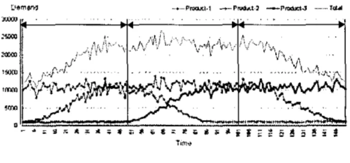
Abstract - Semiconductor manufacturing technology is In Fig. 1, we simulate the 128Mb, 256Mb and 512Mb DRAM progressing rapidly. As shown by the celebrated Moor’s laws.

new generations of semiconductor products emerge in the generations ofien CO-exist in the same fabrication facility. For wll

effective manufacturing resource planning, accurate 2tmD

prediction of product m u is therefore crucial. Product-mix x m

prediction is usually made by performing the demand :uu

disaggregation function in demand planning. In this paper, ,mm weighted product-mu estimation methodologies are first lm proposed. Dynamic weighting schemes are then developed to

methodologies will be rested with simulated DRAM demands and actual semiconductor demands of different technology generations.

demands to resemble these three characteristics.

pace of every 6 months. A s a result, technologies of different ~ e m m -.-Prmut,., -..“-, -n-J ...* I

improve the accuracy of product mix prediction. The Tl”0

Fig. 1 Simulated DRAM demands

INTRODUCTION

Results of demand planning serve as the basis of every planning activity in the supply network and ultimately determine the effectiveness of manufacturingllogistic operations in the network. A common demand planning approach is to make forecast at an aggregated level first, and then break down (disaggregate) the forecast statistically and/or judgmentally into the individual forecasts. This is known to be an effective means for better forecasting because the aggregated product-group demand is observed to fluctuate less and easier to make forecast. This approach, however, requires an accurate product-mix prediction to break down the aggregated demand forecast into individual product forecasts. Product-mix can be expressed as demand proportions in a product group. For example, proportions of 64M, 128M and 256111 DRAM demands form the product-mix of the DRAM product group. Thus, product-mix estimation is equivalent to demand disaggregation. That is, to estimate the product-mix, we need to estimate the proportions of individual demands in the product group.

It can he seen, substitution of phasing out product demand by the emerging product leads to dramatic change of product- mix. It is difficult to estimate the product-mix without considering the product life cycles and substitutability. In this paper, we first propose weighted product-mix estimation methodologies. Dynamic weighting schemes are then developed to more effectively capture the PLC for better product-mix prediction. Finally, both simulated DRAM demands and actual semiconductor demands of different technology generations are used to test the proposed methodologies.

WEGHITED PRODUCT-MIX ESTIMATION Among the many product-mix estimates (or demand disaggregation methods) [I], the following two methods are most widely used:

dit

c-

,=I Dt Method A:

ii

=

-

n

An effective product mix estimate should take into consideration the characteristics of semiconductor demands.

There are three important characteristics that will be

2

di,

5

Dr MethodB:

ii

=f=l

~

where di, is the demand of product i at period 1; is the number of historical demand periods;

D,

=

I d i t

is the total

considered in our proposed methodologies: n

/,=,

n (1)

1. Product substitutability: most products within the same

product group are substitutable among one another. k

2. Product life cycle (PLC): Fast-paced technology i=l

demand at period I ; k is the number of products in the product develonment leads to fast PLC transition.

group; and

k.

is the mean-proportional estimate of product i. 3. Variability proportional to volume: the greater the demand

volume, the more volatile the demand.

As mentioned earlier, directly forecasting on individual product demands usually result in a far-off forecast that not only impairs the quality of subsequent manufacturing plans but also send the ripples to the down-stream manufacturing activities via the supply chain. To capture the effect of PLC change on the product-mix, we would give higher weights to the more recent data; that is, we like to have the product-mix estimate more influenced by more recently observed demands.Thus, we apply exponential weights to the product- mix estimates in ( I ) , (7), and (13), respectively, to obtain product-mix prediction for the next time period. First, the mean-proportional estimate in ( I ) now becomes an exponentially weighted averagc of historical demands:

where

bi,,7+l

is the prediction of product i proportion for period n C l ; and w,,is the weight applied to product i demand at time I and satisfies:

n

(3)

fl ai(l-ni)"-'

2

WiI =

c

= I

I=I

with the constant

a,

to control the declining rate over time as

shown in Fig. 2. I=I 1 - (1 - a i ) "

I.,*",.

Fig. 2 Exponential weights controlled by

a

values How to choose appropriate a, values in (3) becomes critical for accurate product-mix estimate.

PLC LEADING INDICATOR

To find the best smoothing constants a, of forecast estimate at period e, that is to find smoothing constants a; (;=I&), we minimize the mean squared forecast errors overs periods:

Determination of good a, is a very time consuming task. Suppose each a, has 99 possible values (ai = 0.01

-

0.99) Then, there are 99' possible (a1 ,az....,ak} candidates. The

time to compute all candidates to search for the best

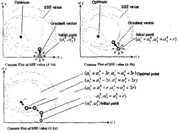
{ a l , a z , ..., a k } to minimize (4) requires enormous computing power, The most common method is Steepest Descent Search [2]. The search of the smoothing constants can be treated as a k-variable (al-& steepest-descent search with (4) as the objective function to minimize. Treat (a,,a2, ..., a b } as a point "d' in k-dimension coordinate system. The steepest- descent search process here can be seen as a process to find the point in the k-dimension coordinate system. Furthermore, the movements of a from one point to another are reached by adjusting each a; with fixed step size "r". There are three possible movements for each ai, adding one step size to

a,,

(a;+r), subtracting one step size from a,, (ar.), nr keep the a,

at the original position. The successive points of (I

representing the most SSE-reduced direction which is called the "gradient vector" while all the other possible directions are called "candidate vectors". Termination of the search occurs at the point where the gradient vector becomes null; i.e., the current a point has the smallest SSE value. An example of two-product steepest-descent smoothing constant search process is shown in Fig. 3.

m h u m

Co"l.uPI*cdEsB~~cu 14.lCI

Fig.3 Two-product steepest-descent search process The steepest descent method is still a computation-intensive method. It would be much more efficient if we know the direction toward the minimum. Taking the effect of changing demand variability into account, we invented a,PLC transition leading indicator using the sample one-lag autocorrelation (SAC) statistic: 1 1-(3-l) - -

c

(4

- 2 ) ( 4 + ,

-4

-

1

(d,

-7y

( 5 ) SAC, =

6

= r=r-I 1 l-(.r-l) s r=1

where SAC, is the one-lag sample autocorrelation calculated at period f using demand dataset {d,_,s+l ,..., d , } . When the product is at the "growth" or "decline" phase, the product-mix proportion significantly rises or falls and the SAC becomes higher as well. If the product is mature in the market and its 85

proportion is stable, SAC will be lower because noise dictates the changes of the product-mix proportion (Fig. 4).

Fig. 4 Relationship among

a ,

SAC and PLC Sample sizes in (5) determines how sensitive the SAC is to the PLC transition and to the demand noise. Fig. 5 shows the SAC values with sample sizes s=15,25 and SO for a simulated DRAM demand.

1.2 - --l( m-tm +Rd".&l O*c7-.il.=w

0.6 -

Fig. 5 SAC calculated by different sample sizes It can be seen that the SAC with a large sample size (s=50) is too slow to reflect the PLC transition while the SAC with small sample size (s=15), though responsive to the PLC transition, is too sensitive

to

the demand

noise.

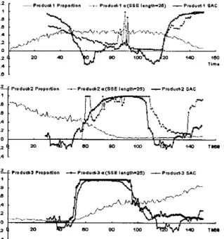
The sample size of 25, approximately on half of one PLC phase, gives the SAC a very good indication of PLC transition.

Fig. 6 shows the smoothing constant estimated by steepest descent search (SDS), SAC calculated with s=25 and the product-mix proportions of the simulated DRAM data (Fig. 1). The smoothing constant estimate goes up when the trend is rising or declining but goes down in the maturity phase. The trend of SAC and the trend of SDS-estimated smoothing constants match each other pretty well. Therefore, SAC would be a good leading indicator to determine the changing trend of the smoothing constants. That is, the smoothing constant estimated at period f + I should be higher than that at period f

when SAC,,, is higher than SAC, and vice versa. Using the SAC as a leading indicator for the search for the best smoothing constants has been proven to cut the computing time to 1/55, Fig. 7 shows the procedure of the prediction scheme.

0 . 4 1

Fig. 6 Smoothing constant estimates and SAC, (DRAM)

START

0 Given the Initial a by Steepest-Descent Search

0 Calculate SAC,

*~

. . . I

\~ ...

0 New data available !

0 Calculate new SAC,., and SAC trend (SAC,,,-SAC,)

Use the SAC trend to estimate the new a at the next period I

i

\, _{... ... ...}

END

Fig. 7 Dynamic product mix estimate scheme

EVALUATION OF PROPOSED METHODOLOGY In order to evaluate the proposed product-mix prediction scheme, we use proportion mean squared error (PMSE):

k+n m

r=k+li=l

PMSE =

z

C(e,,,

-

e,,)2

as the evaluation measure and compare the performance against two conventional proportion estimate methods: methods A and B.

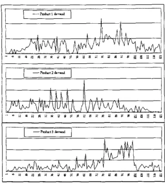
In addition to the simulated DRAM demands, actually semiconductor demand data as shown in Fig. 6 is also tested.

Fig. 8 Actual semiconductor demands

It is diffcult to observe the relationship among the three individul demands from Fig. 8. However, the product-mix proportions (Fig. 9) show clearly the relationship among these three products.

I

I n

' I I !

The results (Table 1 ) show significant improvements by the proposed method (PLC Indicator Dynamic EWMA, PIDE) in both the simulated and actual demand cases.

Actual D a t a

T o t a l P M S E

I

C o n ~ e n f i o n a l M e l h o d I

1

Table 1 Evaluation Results

ACKNOWLEDGEMENT

This research is supported in part by ISMT and SRC (879.001) and by NSC (NSC90-2218-E-002-046).

REFERENCE

[l] Charles W. Gross and Jeffrey E. Soh1 "Disaggregation Methods to Expedite Product Line Forecasting" Journal of Forecasting, Vol. 9,233-254, 1990

[2] Ward Cheney and David Kincaid, Numerical Mathematics and Computing, 41h edition, Brooks/Cole Publishing Company, 1999

AUTHOR BIOGRAPHY

Argon Chen is a faculty member of the Graduate Institute of Industrial Engineering at National Taiwan University (NTU). He received his Ph.D. degree in industrial engineering and earned his M.S. degrees in industrial engineering and in statistics from State University of New Jersey, Rutgers. Dr. Chen has been working closely with the semiconductor industry in Taiwan as a principle investigator of several research projects. In 2001, Dr. Chen was awarded a 3-year research project co-funded by Semiconductor Research Corporation (SRC) and International Sematech (ISMT). Dr. Chen published his research work mostly in IEEE Transactions on Semiconducfor Manufacturing and Technometrics.

Fig. 9 Product-mix of actual semiconductor demands