分散式系統之自我穩定極小控制集演算法與凱氏圖之正負號星控制數

(1)

國立交通大學

應用數學系

博士論文

分散式系統之自我穩定極小控制集演算法

與凱氏圖之正負號星控制數

Self-stabilizing Minimal Dominating Set Algorithms of

Distributed Systems and the Signed Star Domination

Number of Cayley Graphs

研究生：邱鈺傑

指導教授：陳秋媛

(2)

分散式系統之自我穩定極小控制集演算法

與凱氏圖之正負號星控制數

Self-stabilizing Minimal Dominating Set Algorithms of

Distributed Systems and the Signed Star Domination

Number of Cayley Graphs

研究生：邱鈺傑 Student: Well Y. Chiu

指導教授：陳秋媛 Advisor: Chiuyuan Chen

國立交通大學

應用數學系

博士論文

A Dissertation

Submitted to Department of Applied Mathematics

College of Science

National Chiao Tung University

in Partial Fulﬁllment of the Requirements

for the Degree of

Doctor of Philosophy

in

Applied Mathematics

July 2014

Hsinchu, Taiwan, Republic of China

(3)

摘要

圖論的控制集問題的研究始於 1960 年代。一個分散式系統 (例

如：一個隨意網路) 可以用一個無向簡單圖 G = (V, E) 來表

示，其中 V 表示點集，而 E 表示點跟點之間的聯結關係。圖

G

的點集 V 的子集合 D 被稱為是控制集，若此子集 D 具有

性質：V 中的任一元素 v 屬於 D 或與 D 中的元素相鄰。如果

一個控制集不真包含另一控制集，則稱其為極小控制集 (簡記

為 MDS)。極小控制集在無線網路中的應用之一是使所需的資

源中心保持為較少數目。

自我穩定是一個可用於設計分散式系統容忍暫時性錯誤的一個

概念，並且是在 1974 年由 Dijkstra 提出。一個分散式系統是

自我穩定的，如果它滿足：不論初始組態為何，系統總是能保

證在有限時間內達到一個合法的 (正確的) 組態。此處所稱的

系統組態是由系統中所有節點的狀態所組成。一個自我穩定演

算法由一些規則所組成，每個規則都有其觸發條件及其對應動

作，該動作能通過更新節點的變數來改變節點的狀態。每執行

一個規則稱為是一步。本論文所提出的演算法的效能皆是以執

行總步數來計算。自我穩定演算法有許多不同的執行模式，且

執行模式是以排程器的概念來呈現。排程器分為公平的及不公

平的兩種。眾所皆知，不公平的分散式排程器比其他類型的排

程器更貼近實際使用狀況。

i

(4)

令 n 表示給定的分散式系統的節點數。在 2007 年，Turau 對

於 MDS 問題，提出了不公平的分散式排程器下的第一個線性

時間的自我穩定演算法，此演算法在最多 9n 步之後穩定。在

2008 年，Goddard 等人改進了上述演算法並做到最多 5n 步。

我們將在本論文中提出一個採用不公平分散式排程器下最多

4n

步的自我穩定 MDS 演算法。

理想中，MDS 演算法是希望能做到 MDS-靜止的，亦即，若分

散式系統的初始組態已經是一個 MDS，則演算法將不執行任

何動作。值得注意的是，在正常模式中，一個節點只能取得其

一步內鄰居的資訊，我們稱這些資訊為 1 步資訊。不幸的是，

在本論文中，我們將證明：1 步資訊不足以建立一個 MDS-靜

止的演算法。在本論文中，我們將討論此一問題，並針對自我

穩定 MDS 演算法提出一個新的性能評量，稱為穩定性。我們

推廣這部份的結果至其他自我穩定演算法，並將自我穩定演算

法分類為四個層次。特別的是，我們將證明：在 2 步資訊模式

下，可建構出自我穩定 MDS-靜止的演算法，且其穩定時間之

上界為 2n 步。

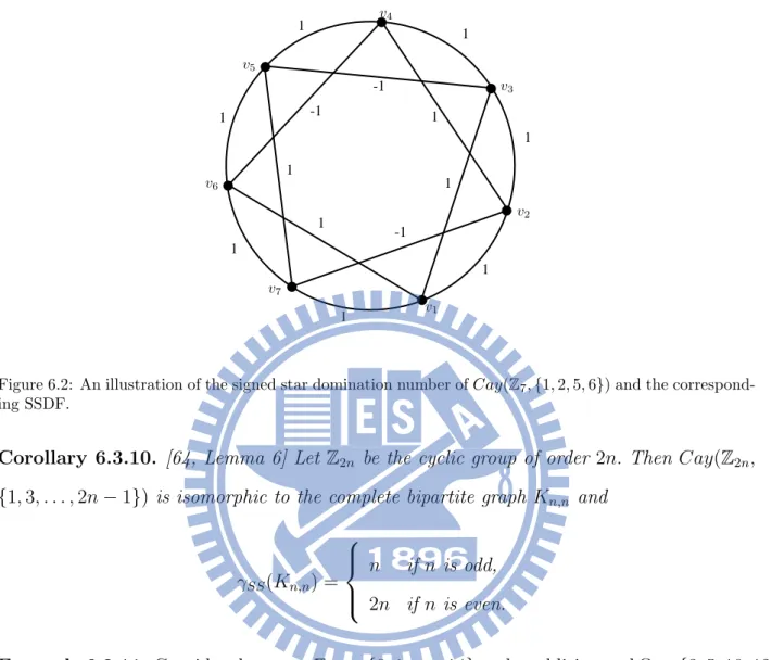
在 2005 年，Xu 提出了圖的帶正負號星控制集的概念，在 2007

年，Wang 給出了完全圖的帶正負號控制數，詳細定義請參見

本論文的第五章。在 2010 年，Atapour 等人定義了帶正負號

星控制劃分數，並利用完全圖具有可完全 1-因子分解或可完全

漢米爾頓圈分解的性質，計算出完全圖的帶正負號星控制劃分

數。在 2012 年，我與印度學者 Chelvam 等人合作，定義了有

向圖的帶正負號星控制數，給出了全部有向凱式圖的帶正負號

星控制數，與無向凱式圖的帶正負號星控制數的部份結果，並

推廣這些結果至可完全

{2, 1}-因子分解的正則圖。

ii

(5)

Abstract

The study of the domination problem in graph theory began in the nineteen-sixties. A distributed system such as an ad hoc network can be modeled by an undirected simple graph G = (V, E), where V represents the set of nodes (i.e., processes) and E represents the set of interconnections between processes of the distributed system. A subset D of the vertex set

V of G is a dominating set if each vertex v ∈ V is either a member of D or

adjacent to a vertex in D. A dominating set of G is a minimal dominating set (MDS) if none of its proper subsets is a dominating set of G. An MDS has an application of clustering in wireless networks and is maintained for minimizing the number of required resource centers.

Self-stabilization is a concept of designing a distributed system for tran-sient fault toleration and was introduced by Dijkstra in 1974. A distributed system is self-stabilizing if, regardless of its initial configuration, the system is guaranteed to reach a legitimate (i.e., correct) configuration in a finite time. Here the system configuration consists of the state of every process. A self-stabilizing algorithm comprises a collection of rules and each rule has a trigger precondition and an action. The action changes the state of the node by updating its variables. An execution of a rule is called a move. The per-formance of the proposed algorithms of this thesis is measured by the total number of moves executed by an algorithm. Various execution models have been used in self-stabilizing algorithms and these are encapsulated with the notion of daemons. A daemon can be fair or unfair. It is well-known that an unfair distributed daemon is more practical than other types of daemons.

(6)

Let n denote the number of nodes (processes) in a given distributed sys-tem. In 2007, Turau proposed the ﬁrst linear-time self-stabilizing algorithm for the MDS problem under an unfair distributed daemon; this algorithm stabilizes in at most 9n moves. In 2008, Goddard et al. improved the re-sult to a 5n-move algorithm. It is interesting to develop an algorithm that takes less moves than the best known result—5n moves using an unfair dis-tributed daemon. In this thesis, we will present a 4n-move self-stabilizing MDS algorithm using an unfair distributed daemon.

It is desired that an MDS algorithm is MDS-silent, which means that if the original conﬁguration of the distributed system is already an MDS, then the algorithm should not make any move. Note that in the normal model, a node can only access the information of its 1-hop neighbors and we call such information distance-1 information. Unfortunately, in this thesis we will prove that distance-1 information is not suﬃcient for building up an MDS-silent algorithm for a distributed system. Therefore it is impossible for an algorithm to be MDS-silent under a normal model, in which only distance-1 information is accessible. What will happen if a node can access the information of its k-hop neighbors for k ≥ 2? In this thesis, we will discuss this problem and propose a new performance measure, called stableness, for self-stabilizing MDS algorithms. We also generalize this result to categorize all self-stabilizing algorithms into four levels. In particular, we will show that a self-stabilizing MDS-silent algorithm can be built up under the distance-2 model and the stabilizing time is upper bounded by 2n.

Let G be a simple connected graph with vertex set V (G) and edge set

E(G). A function f : E(G) → {−1, 1} is called a signed star dominating

function (SSDF) on G if ∑_e_∈E(v)f (e) ≥ 1 for every v ∈ V (G), where E(v)

is the set of all edges incident to v. The signed star domination number of

G is deﬁned as γSS(G) = min{

∑

e∈E(G)f (e)| f is an SSDF on G}. Let D

be a ﬁnite digraph with vertex set V (D) and arc set A(D). For each vertex

v ∈ V (D), let A(v) be the set of all out-going arcs from v. By replacing E(v)

by A(v), one can deﬁne SSDF on D and γSS(D) = min{

∑

a∈A(D)f (a) | f is

(7)

an SSDF on D}. Let Γ be a ﬁnite nontrivial group and S be a nonempty subset of Γ. The Cayley digraph CayD(Γ, S) is the digraph whose vertices

are the elements of Γ, and there is an arc from α to ασ whenever α_{∈ Γ and}

σ ∈ S. Let Ω be a symmetric generating subset of nonidentity elements of Γ.

The Cayley graph Cay(Γ, Ω) corresponding to Γ and Ω is the ordinary graph with vertex set Γ and edge set E =_{{{α, ασ} | α ∈ Γ, σ ∈ Ω}. In this thesis,} we obtain exact values for the signed star domination number of all Cayley digraphs CayD(Γ, S) and certain classes of Cayley graphs Cay(Γ, Ω), which

is later generalized to{2, 1}-factorable graphs. Note that these solutions are from a joint work with Chelvam and Kalaimurugan.

(8)

Acknowledgments

由衷感謝兩大貴人：我的指導教授陳秋媛老師與我未來的老婆

陳怡樺。

(9)

List of Tables

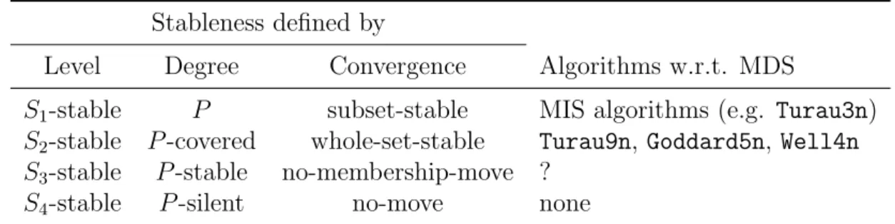
3.1 Self-stabilizing algorithms for the minimal dominating set problem. . . 17 4.1 The levels of stableness and convergence of self-stabilizing algorithms. . . 40 4.2 Self-stabilizing MDS algorithms on general graphs with diﬀerent levels of

stableness. . . 40 4.3 Self-stabilizing independent set algorithms. . . 46 4.4 Self-stabilizing dominating set algorithms. . . 47

(13)

List of Figures

3.1 The state diagram of Well4n. . . 24 3.2 The average number of moves made by Well4n, Goddard5n, and Turau9n with

regard to the transmission ranges, where the vertical line segments denote the standard deviations. . . 29 3.3 The average number of membership moves made by Well4n, Goddard5n, and

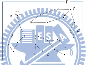
Turau9n in terms of the transmission ranges, where the vertical line segments denote the standard deviations. . . 30 4.1 The transition diagram of a distributed system. The structures of a loop, a

path, a tree, and a 3-cycle are shown in the areas a to d, respectively. Area

e depicts a node with out-degree 3; this node denotes a conﬁguration with

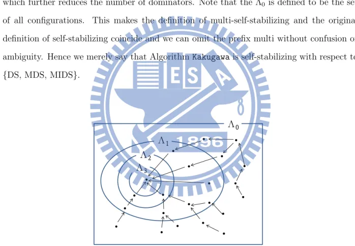
three possible following conﬁgurations. . . 36 4.2 The transition diagram of the algorithm Kakugawa. A dominating set (DS)

is feasible and a minimal dominating set (MDS) is optimal. The algorithm converges to a single point, which is the lexicographically ﬁrst minimal inde-pendent domination set. . . 44

(14)

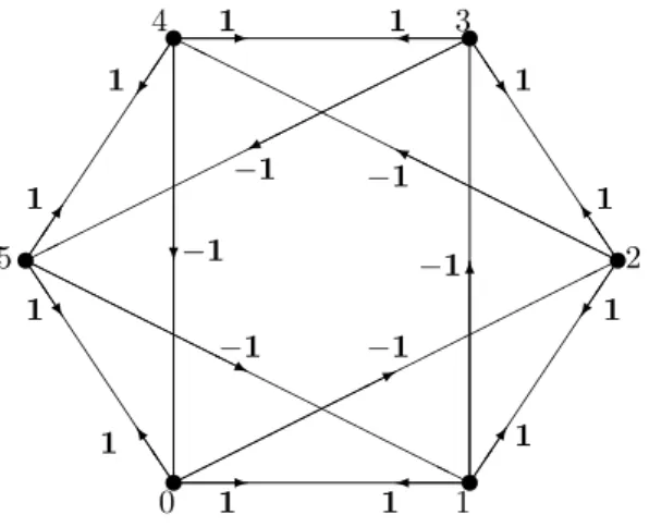
4.3 The transition diagram of a multi-self-stabilizing system with respect to three layers of legitimacy. . . 45 6.1 An illustration of the signed star domination number of CayD(Z6,{1, 2, 5})

and the corresponding SSDF. . . 59 6.2 An illustration of the signed star domination number of Cay(Z7,{1, 2, 5, 6})

and the corresponding SSDF. . . 64 6.3 An illustration of the signed star domination number of Cay(Z15,{3, 5, 10, 12})

(15)

List of Algorithms

1 Dijkstra . . . 10 2 Turau3n . . . 19 3 Turau9n . . . 20 4 Goddard5n . . . 21 5 Well4n . . . 23 6 Kakugawa . . . 43 7 Well2n . . . 51

(16)

Chapter 1 Introduction

Graph theory has multiple applications in the real world. In this thesis, we consider a distributed system whose topology is represented by an undirected simple graph G = (V, E), where V represents the set of nodes (i.e., processes) and E represents the set of edges (i.e., the interconnections between processes) of the distributed system. We discuss the problem of developing efficient stabilizing minimal dominating set algorithms, the existence of self-stabilizing minimal dominating set algorithms with respect to different levels of stableness, and finding the signed-star domination number of graphs. Throughout this thesis, we use the terms “vertex” and “node” interchangeably, and we use the terms “distributed system” and “graph” interchangeably. Also, unless otherwise specified, all graphs are assumed to be simple.

1.1 Basic graph definitions

A graph G is a nonempty ﬁnite set V along with a ﬁnite set E of 2-element subsets of V . The elements of V are called vertices and the elements of E are called edges. The number of elements in a set S is called the cardinality of S and is denoted by |S|. We use n and

(17)

CHAPTER 1. INTRODUCTION 1.1. BASIC GRAPH DEFINITIONS

m to denote the order and the size of a graph, respectively; that is, n =|V | and m = |E|.

An edge with endpoints u and v is denoted as uv. Two vertices u and v in V are said to be adjacent in G, denoted by u ∼ v, if there exists an edge uv ∈ E. Let v ∈ V . A vertex

u is a neighbor of v if they are adjacent. The open neighborhood (or shortly, neighborhood )

of v is the set of vertices to which v is adjacent; that is, N (v) := {u ∈ V | u ∼ v}. The

degree of a vertex v is deﬁned as deg(v) :=|N(v)|. We use the notation N[v] = N(v) ∪ {v}

to denote the closed neighborhood of v. The deﬁnition of the maximum degree ∆ of G is ∆(G) := max{deg(v) | v ∈ V }. We deﬁne the diameter of G to be max{d(u, v) | u, v ∈ V } and the radius of G to be min{max{d(u, v) | v ∈ V } | u ∈ V }.

The length of a path or a circle is deﬁned to be the number of edges in the path or the circle. The distance between any two vertices u and v in G, denoted as d(u, v), is the length of a shortest path between u and v in G. A vertex u is called a k-neighbor of a vertex v if

d(u, v) = k. The (open) k-neighborhood Nk(v) of vertex v is the set of vertices u such that

1≤ d(u, v) ≤ k. The closed k-neighborhood Nk[v] of vertex v is Nk(v)∪{v}. For a vertex set

S, Nk(S) =

∪

i∈SNk(v). Conventionally, the subscript k is omitted if k = 1, as a neighbor

of v or the neighborhood N (v).

To color the vertices in a graph G = (V, E) is to give each vertex a positive integer color value in such a way that no two adjacent vertices get the same color. In many practical considerations, it is desirable to minimize the number of colors used. If at most k colors are used, the result is called a k-coloring. The smallest possible positive integer k for which there exists a k-coloring of G is called the chromatic number of G and is denoted as χ(G).

Given an undirected graph G = (V, E), a matching is deﬁned to be a subset M ⊆ E such that for all nodes v ∈ V at most one edge of M is incident with v. A matching M is

maximal if there does not exist another matching M′ such that M ⊂ M′. A subset M ⊆ E is called a k-matching of G if|E(v) ∩ M| ≤ k for all nodes v ∈ V , where E(v) is the set of edges incident from v. Note that a 1-matching is a simple matching.

(18)

CHAPTER 1. INTRODUCTION 1.2. GRAPH DOMINATION AND RELATED DEFINITIONS

A vertex cover for a graph G = (V, E) is a subset C ⊆ V such that, for each edge uv ∈ E, at least one of the two endpoints u and v belongs to C.

1.2 Graph domination and related definitions

Although the study of the graph domination problem began in the nineteen-sixties, the ﬁrst paper which addresses the queens dominating chessboard problem dates back to 1862. Given an undirected graph G = (V, E), a dominating set D is a subset of V such that

N [v]∩ D ̸= ∅ for every v ∈ V . We say a node in D dominates its neighbors and a node

in V\D is dominated if it has a neighbor in D. Nodes in the dominating set D are called

dominators, and nodes not in D are called dominatees.

A dominating set D of G is a minimal dominating set (MDS) if D does not properly contain another dominating set of G. The MDS problem is that of finding a minimal domi-nating set for any given undirected graph G and this is the problem discussed in this thesis. A dominating set D of G is a connected dominating set (CDS) if the subgraph of G induced by D is connected; minimality is defined similarly. The problem of finding a minimum connected dominating set is known to be NP-complete [22].

Dominating sets are closely related to independent sets. In an undirected graph G = (V, E), a subset I ⊆ V is independent if no two nodes in I are adjacent. An independent set

I of G is a maximal independent set (MIS) if it is not a proper subset of any independent

set of G. It is well-known that a maximal independent set of G is a dominating set of G. Therefore a maximal independent set of G is also called an independent dominating set of

G. The independent set problem is the optimization problem of ﬁnding an independent set

of maximum cardinality in a graph. The independent set problem is NP-complete [22]. Given a non-negative integer k, we deﬁne a k-cluster of G to be a nonempty subgraph of G of radius at most k. If C is a k-cluster of G, we say that v ∈ V (C) is a clusterhead of

(19)

CHAPTER 1. INTRODUCTION 1.2. GRAPH DOMINATION AND RELATED DEFINITIONS

C if, for any u∈ V (C), there is a path of length at most k in C from v to u. We deﬁne a k-clustering of G to be a set {C1, . . . , Cℓ} of k-clusters of G such that every vertex v ∈ V

lies in exactly one of the Ci. A set of vertices D⊆ V is a k-dominating set of G if, for every

v ∈ V , there exists u ∈ D such that d(u, v) ≤ k. Building a k-dominating set in a graph is

useful because it allows to split the graph into k-clusters. We say that a k-dominating set

D is minimum if no k-dominating set of G has fewer dominators than D. The problem of

ﬁnding a minimum k-dominating set is known to be NP-hard [22].

Now, we deﬁne the problem of computing an MDS in distributed systems. Let G = (V, E) be a graph that represents a distributed system. By v.id, we denote the process identiﬁer of

v for each process v of the distributed system. In discussing the process identiﬁer, we can

use v to denote v.id when it is clear from contexts. For a distributed system, the minimal

dominating set problem is deﬁned as follows:

• For each process v ∈ V , its identiﬁer and its neighbors are given as an input. • Each process v ∈ V must decide its decision dv as an output.

• The set {v ∈ V : dv = 1} must be an MDS.

The decision dv of v can be encoded by the local state qv of v in an arbitrary way by an

algorithm. Formally, dv ≡ Dec(qv) for some decoding function Dec on the local states deﬁned

by an algorithm.

In summary, given an undirected graph G = (V, E), a subset S of V is:

• independent if for each pair i, j ∈ S, ij ̸∈ E;

• dominating if for every i ∈ V , either i ∈ S or i ∈ N(S);

• maximal independent if S is independent and any subset properly containing S is

(20)

CHAPTER 1. INTRODUCTION 1.3. APPLICATIONS OF GRAPH DOMINATION

• minimal dominating if S is dominating and no proper subset of S is dominating.

1.3 Applications of graph domination

A minimal dominating set needs to be maintained to optimize the number and location of resource centers in a network [35]. Some applications of this area include school bus routing, computer communication networks, resource allocation schemes, radio stations with limited broadcasting range, etc. An important concept in the study of a vertex subset problem is the difference between a “minimum” and a “minimal” set with a given property. To find a minimum cardinality of dominating set is hard, but we can easily find a minimal dominating set in polynomial time in a distributed manner.

Specifically, a minimal dominating set can be usefully applied in wireless sensor networks. One way to find a connected dominating set is to firstly find a minimal dominating set and then connect each dominator by including more nodes into the dominating set. A connected dominating set of a communication graph can serve as the virtual backbone for supporting the communication between sensors in a wireless sensor network. This is because its domination property ensures that every node is either in the backbone or adjacent to a node in the virtual backbone, and its connectivity property guarantees that any two nodes can send messages to each other via a series of intermediate nodes in the virtual backbone. In a connected component of a wireless sensor network’s communication graph, sensors are linked with one another so that they can interchange messages and deliver messages along a simple path to make the communications between non-adjacent sensors become possible.

(21)

CHAPTER 1. INTRODUCTION 1.4. THESIS OUTLINE

1.4 Thesis outline

This thesis is organized as follows. Chapter 2 gives the fundamentals of self-stabilizing algorithms on a distributed system. Self-stabilization is a concept of designing a fault-tolerant distributed system for a finite number of transient faults, such as message loss and memory corruption. The concept of self-stabilization was first proposed by Dijkstra in 1974 [15]. The configuration, also called the global state, of a distributed system consists of the state of every node and the content of every communication channel. Given an illegal starting configuration, such a system has to be able to reach a legal configuration in a finite time. Once in a legal configuration, the system may only move to another legal configuration if there is no external interference. The concept of self-stabilization has been proven to be an effective and cost-effective paradigm for localized state-based computation to implement distributed algorithms, especially in networks with resource-constrained nodes like sensor networks or ad hoc networks. The objective of self-stabilization is to recover the system from failure in a reasonable time and without intervention by any external agency.

The purpose of Chapter 3 is to discuss the problem of designing eﬃcient self-stabilizing algorithms for the minimal dominating set problem. We consider a distributed system whose topology is represented by an undirected graph G. The MDS problem is to ﬁnd a minimal dominating set for the given undirected graph G. Let n denote the number of nodes in the system. The main contribution of this chapter is to propose a (4n− 2)-move self-stabilizing algorithm for the MDS problem under an unfair distributed daemon. We also compare our algorithm with other self-stabilizing algorithms in this chapter.

The purpose of Chapter 4 is to discuss the levels of stableness of self-stabilizing al-gorithms for the MDS problem. Obviously, a node in a distributed system has limited information about the whole system. Usually, a node can only access the information of nodes in its 1-neighborhood. Let k be a positive integer. We say a distributed system is

(22)

CHAPTER 1. INTRODUCTION 1.4. THESIS OUTLINE

in the distance-k model if a node in the system can access the information of nodes in its

k-neighborhood. For convenience, we say a distributed system is in the normal model if it is

in the distance-1 model. What will happen if a node can access the information of nodes in its k-neighborhood for k≥ 2? In this chapter, we discuss the above problem and propose a new performance measure, called stableness, for self-stabilizing MDS algorithms. We deﬁne

MDS-silent algorithms and MDS-stable algorithms, and we classify four levels of stableness

for self-stabilizing algorithms.

It is desired that an MDS algorithm is MDS-silent, meaning that if the original conﬁgu-ration is already an MDS, then the algorithm should not make any moves. In Chapter 5, we discuss the problem of designing a self-stabilizing MDS-silent algorithm. In the distance-2 model, a node can instantaneously access the information of all nodes within distance two from it. The main contribution of this chapter is to propose a (2n− 1)-move self-stabilizing MDS-silent algorithm for the MDS problem under an unfair distributed daemon in the distance-2 model.

The purpose of Chapter 6 is to ﬁnd out the signed star domination number (a variant of the domination number) of Cayley digraphs and Cayley graphs. A function f : E(G)→

{−1, 1} is called a signed star dominating function (SSDF) on G if∑e∈E(v)f (e)≥ 1 for every

v ∈ V (G), where E(v) is the set of all edges incident with v. The signed star domination number of G is deﬁned as γSS(G) = min{

∑

e∈E(G)f (e)| f is an SSDF on G}. In Chapter 6,

we obtain exact values for the signed star domination number for certain classes of Cayley digraphs and Cayley graphs.

(23)

Chapter 2 Self-stabilization

The concept of self-stabilization was first proposed by Dijkstra [15] in 1974. This concept has been proven to be an effective and cost-effective paradigm for localized state-based computation to implement distributed algorithms, especially in networks with resource-constrained nodes like sensor or ad hoc networks. The objective of self-stabilization is to recover the system from failure in a reasonable time and without intervention by any external agency. Self-stabilization is based on two basic ideas: (i) the code executed by a node is incorruptible (as if written in a fault-resilient memory) and transient faults affect only data values; (ii) the goal system behavior can be checked by evaluating some predicates of the system state variables.

This chapter is organized as follows. Section 2.1 gives the early draft of self-stabilizing systems. Section 2.2 states the fundamental concepts of self-stabilizing systems. Section 2.3 introduces various execution models which are encapsulated with in the notion of daemons and fairness. Section 2.4 gives a brief review of self-stabilizing algorithms on graphs (span-ning tree construction, independent sets, dominating sets, and so on). An application of self-stabilizing algorithms to wireless sensor networks is given in Section 2.5.

(24)

CHAPTER 2. SELF-STABILIZATION 2.1. THE EARLY DRAFT OF SELF-STABILIZING SYSTEMS

2.1 The early draft of self-stabilizing systems

Self-stabilization is a concept of designing distributed systems for transient fault toleration. The original idea of self-stabilization was introduced by Dijkstra in a seminal paper in 1974 [15]. The earliest deﬁnition of a self-stabilizing system requires that:

(i) in each legitimate (i.e., legal) state, one or more privileges will be present;

(ii) in each legitimate state, each possible move will bring the system again in a legitimate state;

(iii) each privilege must be present in at least one legitimate state; and

(iv) for any pair of legitimate states, there exists a sequence of moves transferring the system from the one into the other.

Dijkstra considered machines placed in a ring, and had chosen the legitimate conﬁgura-tion in which exactly one privilege is present. Imagine there is a group of people sitting in a circle. If they want to speak, they have to raise their hands and wait for calls. A central chairman chooses a person to speak once at a time. In a while, the situation becomes stable: exactly one person raises his or her hand and is chosen to speak.

Three solutions were given. The ﬁrst one with K-state machines is easy since K is larger than the number n of machines. The second one is a solution with four-state machine. The most complicated one with three-state machines is shown in Algorithm 1. These algorithms are correct: in a ﬁnite time, exactly one privilege will be present.

2.2 Fundamental concepts of self-stabilizing systems

In spite of the fact that the concept of self-stabilization was introduced by Dijkstra in 1974 [15], serious work only began in the late nineteen-eighties. See Dolev’s book for an overview

(25)

CHAPTER 2. SELF-STABILIZATION 2.2. FUNDAMENTAL CONCEPTS OF SELF-STABILIZING SYSTEMS

Algorithm 1 Dijkstra

variables

Mi.S ∈ {0, 1, 2} with addition taken modulo 3;

for the machine M0

if M0.S + 1 = M1.S then M0.S := M0.S + 2;

for the machine Mn−1

if Mn−2.S = M0.S and Mn−2.S + 1 ̸= Mn−1.S then Mn−1.S := Mn−2.S + 1;

for the other machines Mi

if Mi.S + 1 = Mi−1.S then Mi.S := Mi−1.S;

if Mi.S + 1 = Mi+1.S then Mi.S := Mi+1.S;

[16].

Self-stabilizing algorithms are speciﬁed as a collection of rules executed on each node. Each rule has a trigger precondition and an action. The precondition of a rule is a Boolean predicate involving the states of the node and its neighbors, and the action changes the state of the node by updating its variables. A rule is enabled if its precondition evaluates to be true. A node is privileged if at least one of its rules is enabled. A node moves by changing state if it is selected by the control scheduler. Therefore the execution of an action is called a move, no matter how many variables it changes in the action.

A fundamental idea of self-stabilizing algorithms is that the distributed system may be started from an arbitrary configuration. After a finite time, the system reaches a correct configuration, called a legitimate configuration. We say that the system has stabilized if no nodes are privileged. An algorithm on a distributed system is called self-stabilizing [15, 16, 18, 65] if the following two properties hold:

Convergence The convergence property ensures that, starting from any illegitimate state, the distributed system reaches a legitimate state in a ﬁnite time without any external intervention.

(26)

CHAPTER 2. SELF-STABILIZATION 2.2. FUNDAMENTAL CONCEPTS OF SELF-STABILIZING SYSTEMS

Closure The closure property ensures that, after convergence, the system remains in the set of legitimate states.

The concept of self-stabilization has been developed for diﬀerent communication styles, and algorithms on a distributed system may assume the inter-node communication mod-els: message-passing model and shared memory model. In communication computer net-works, computers communicate by exchanging messages, which is called the message-passing

model. In the message-passing model, asynchronous computers sending and receiving

mes-sages through ﬁrst-in ﬁrst-out (FIFO) queues which may cause message losing. Other dis-tributed systems usually use the shared memory model of communication, where neighboring communicating entities may communicate via common variables or registers. We distinguish two variants of the shared memory models. The link-register model is associated with a mul-tiprocessor computer or a multitasking single computer, in which each processor/process can communicate with each other only by using separate registers. By using a global clock pulse, writing in and reading from the shared memory of two or more neighboring entities can be synchronized without losing information. The other is the state reading model, which is wildly used in the communicating graph algorithms. In the state reading model, each node can directly read the internal states of its neighboring nodes. Our algorithms assume the state reading model of communication.

Nodes in a distributed system can be modeled as state machines performing a sequence of steps. More precisely, we use composite atomicity, meaning that a node may read all its input variables, perform a state transition, and write all its output variables in a single atomic step. We assume that rules are atomically executed, that is, the evaluation of a precondition and the move are performed in one atomic step. All of the self-stabilizing algorithms presented in this thesis are concerned with composite atomicity and the state reading model unless otherwise speciﬁed. Note that the weakest communication model with register is known as the read/write atomicity model where a process can only atomically

(27)

CHAPTER 2. SELF-STABILIZATION 2.3. DAEMONS AND FAIRNESS

read the state of its neighbors or update its own state [18].

When estimating the time complexity of a self-stabilizing algorithm, we consider the stabilization time not the running time, since a self-stabilizing algorithm is usually a do forever loop and it does not terminate. The stabilization time of a self-stabilizing algorithm is the maximum amount of time it takes for the system to reach a legitimate conﬁguration. The stabilization time is estimated in terms of time-steps or in terms of rounds. A time-step of a system is the amount of time in which a process can make an atomic step. A round is a minimal sequence of time-steps where every process privileged at the start is either tapped or sees its move disabled by the move of a neighbor. In general, the number of time-steps is bounded above by the number of moves.

We assume in a self-stabilizing algorithm, each node maintains its local variables and can make up decisions based on its local variables and its neighbor’s local variables. A node can change its state by making a move, that is, by changing the value of at least one of its local variables. In this thesis, we will follow the conventions used in [30, 34, 75]. In particular, every node executes the same set of rules, and maintains and changes its own state based on its current state and the states of its neighbors [66]. These algorithms can be implemented on wireless sensor networks by using the beacon messages [30]. During the execution, every sensor node broadcasts its state to its neighbors after every change of the state.

2.3 Daemons and fairness

Various execution models have been used in self-stabilizing algorithms and these are encapsu-lated within the notion of daemons (or schedulers). Under diﬀerent daemons, the algorithms diﬀer greatly. Three commonly used daemons are: distributed daemon, synchronous dae-mon, and central daemon. In order to consider the worst-case scenario, a self-stabilizing algorithm is assumed to face an adversarial daemon. The central daemon picks up only

(28)

CHAPTER 2. SELF-STABILIZATION 2.3. DAEMONS AND FAIRNESS

one privileged node to execute an atomic step at each time-step. If a synchronous daemon is supposed, then all the privileged nodes execute an atomic step at each time-step. The

distributed daemon chooses an arbitrary subset of the privileged nodes to execute an atomic

step at each time-step. For the synchronous daemon, the measures time-steps and rounds coincide.

A scheduler can be fair or unfair. A fair daemon guarantees that every node is eventually selected to make a move. Otherwise it is unfair. If a daemon is unfair, then a round is not guaranteed to finish. It is well-known that an unfair distributed daemon is more practical than the other types of daemons and it is the daemon used by our algorithms and by [30, 75]. A distributed algorithm is said to be uniform if all of the individual processes run the same set of rules. If all processes run the same set of rules except a single process, called the root or the leader, then the algorithm is semi-uniform. When algorithms are designed for anonymous systems, the processes do not have any identification [67]. Some algorithms assume that processes have globally unique identifiers. Also, when a process can make moves with random outputs, the algorithm is said to be probabilistic (or randomized); otherwise it is deterministic. A distributed algorithm is dynamic if it can tolerate changes in the topology of the system during its execution. In [18] it is pointed out that self-stabilizing uniform algorithms designed for systems of arbitrary topology are dynamic.

Symmetry breaking is essential for algorithms in distributed systems assuming syn-chronous or distributed daemons [46]. For some problems it has been shown that determin-istic uniform self-stabilizing algorithms are impossible for an anonymous system because the difficulty encountered in symmetry breaking [68]. We assume that each node is designated a unique numeric identifier (ID) so that two neighboring nodes can compete against each other by comparing their IDs. It is to be noted that most self-stabilizing algorithms actually only require locally unique identifiers (i.e., no closed neighborhood contains two identical identifiers). We denote by v.id the identifier of a node v, or by v itself if no ambiguity is

(29)

CHAPTER 2. SELF-STABILIZATION 2.4. SELF-STABILIZING ALGORITHMS ON GRAPHS

caused.

2.4 Self-stabilizing algorithms on graphs

Graph algorithms have natural applications to networks and distributed systems since graphs can be used to model networks or distributed systems. For example, dominating sets are suitable for cluster formation. Colorings are used in mutual exclusion and resource allocation problems. Spanning trees are used in tasks like routing and broadcasting, while matchings can be used in situations of communication where a node must be coupled with exactly one of its neighbors. Thus, many distributed graph algorithms have been developed to be used in network protocols or distributed systems.

Since the publication of Dijkstra’s pioneering paper, lots of self-stabilizing algorithms for a variety of problems have been proposed in the literature. Here, we are interested in the category of graph theoretic problems, which has been deeply investigated since nineteen-nineties. Self-stabilizing algorithms for a variety of graph theoretic problems have been published in recent years. Some problems such as spanning tree construction [2, 6, 10, 23, 39, 63, 69, 71, 73], independence [21, 30, 32, 36, 45, 66, 67, 75], domination [4, 21, 28, 29, 30, 36, 43, 44, 50, 51, 75, 76, 83], coloring [24, 26, 38, 41, 42, 48, 53, 56, 59, 70, 72, 77], and matching [8, 27, 37, 40, 57, 58] have received more attention than other problems such as ﬁnding centers [5], vertex covering [54], clustering [13], etc.

In a graph algorithm for ﬁnding a vertex subset such as the MDS or MIS, the states of processes are categorized into two types. The ﬁrst type is IN, with which the process is considered in the set S with the desired property (MDS or MIS). On the other hand, if the process is considered not in S, then we say it is OUT. The nodes are referred to as IN nodes and OUT nodes according to their states. A neighbor is an IN (resp., OUT) neighbor if it is an IN (resp., OUT) node.

(30)

CHAPTER 2. SELF-STABILIZATION 2.5. APPLICATIONS TO WIRELESS SENSOR NETWORKS

In such a setting when a node makes an execution and therefore changes the values of its variables, we will say it makes a move. A membership move is a move such that the state of the node changes from IN to OUT or from OUT to IN after the execution. An MDS of a distributed system consists of the set of IN nodes after the algorithm stabilizes. If the system is self-stabilizing with respect to MDS, one must show that the convergence and closure properties both hold. While self-stabilizing algorithms exist for computing an MDS, no self-stabilizing algorithm is known to compute a minimal CDS; the predicate seems to be locally non-computable, due to its nature of global predicates [33].

2.5 Applications to wireless sensor networks

Self-stabilization has applications to wireless sensor networks (WSNs). In a wireless system, sensor nodes broadcast their local states to neighbors after each move. The asynchronous execution of an algorithm in each sensor node can be described as of an unfair distributed daemon independently selects a nonempty subset of privileged nodes. The sensor nodes in the network are inﬂuenced by the natural forces which make them mobile. A sensor node would be dead when its limited battery power depletes and if this happens then it leaves the WSN. Hence the topology of a WSN may change frequently. A WSN can model by a distribution system and each node maintains its own neighbor list and can communicate to neighbors via broadcasting messages. When the topology of the system changes, we say an external interference occurs and the system is not stable any more, thus we need a self-stabilizing algorithm to recover the system from an illegitimate conﬁguration.

(31)

Chapter 3 Self-stabilizing MDS algorithms

In this chapter, we consider a distributed system whose topology is represented by an undi-rected, simple graph G = (V, E). Let n denote the number of nodes in the system. Assume each node can read the local state of its neighboring nodes in G. The MDS problem is that of ﬁnding a minimal dominating set in any given graph G and this is the problem concerned in this chapter. The main contribution of this chapter is to propose a (4n− 2)-move self-stabilizing algorithm for the MDS problem under an unfair distributed daemon. A preliminary version of this chapter appeared as [12].

This chapter is organized as follows. In Section 3.1, we give previous results in self-stabilizing MDS algorithms. Section 3.2 presents a (4n− 2)-move self-stabilizing algorithm called Well4n for the MDS problem. Section 3.3 proves the correctness and convergence properties of Well4n and gives an upper bound of 4n− 2 moves. Simulations in average analysis of our algorithm and comparisons with other linear-move MDS algorithms are given in Section 3.4.

(32)

CHAPTER 3. SELF-STABILIZING MDS ALGORITHMS 3.1. PREVIOUS RESULTS

3.1 Previous results

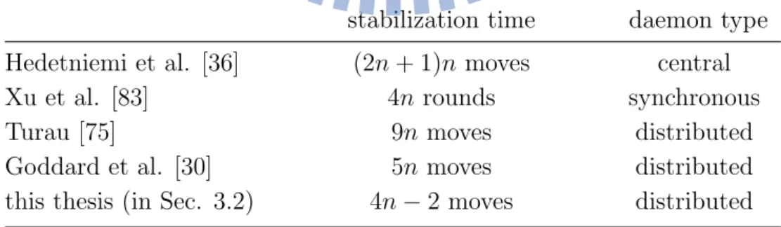
In [36], Hedetniemi et al. proposed the ﬁrst self-stabilizing algorithm for the MDS problem; their algorithm assumes the central daemon. In [83], Xu et al. presented an algorithm under the synchronous daemon. In [75], Turau proposed a 9n-move algorithm under an unfair distributed daemon; this algorithm is the ﬁrst linear-time self-stabilizing algorithm for the MDS problem. In [30], Goddard et al. presented a 5n-move algorithm. A good survey for the self-stabilizing algorithms for the MDS problem can be found in [34].

For simplicity of notation in the context, we say that a conﬁguration conforms to MDS if the set of IN nodes is an MDS of G; otherwise the conﬁguration violates MDS. The time complexity of a self-stabilizing algorithm is estimated in terms of moves or in terms of rounds. As was mentioned in the literature, for a wireless system with bounded resources, the number of moves is at least as important as the number of rounds. The reason is that a node has to broadcast the state to its neighbors after taking a move and therefore a reduction of the number of moves prolongs the lifetime of a network. In the paper [83], Xu uses the number of rounds to estimate the time complexity; but [30, 36, 75] and this thesis use the number of moves. All the known results are summarized in Table 3.1.

Table 3.1: Self-stabilizing algorithms for the minimal dominating set problem.

stabilization time daemon type Hedetniemi et al. [36] (2n + 1)n moves central Xu et al. [83] 4n rounds synchronous Turau [75] 9n moves distributed Goddard et al. [30] 5n moves distributed this thesis (in Sec. 3.2) 4n− 2 moves distributed In the following, we review algorithms in the previous results.

(33)

3.1.1 The first self-stabilizing MDS algorithm

In [36], Hedetniemi et al. proposed the ﬁrst MDS self-stabilizing algorithms. Under a central daemon, the conﬁguration of a graph stabilizes in O(n2_{) moves. In their MDS algorithm,}

every node has two variables: a Boolean variable indicating its state is IN or OUT, and a pointer pointing to one of its neighbors. For convenience, the neighbors of state IN are called IN neighbors. A node will point to the unique IN neighbor, otherwise it will point to null. A node is allowed to enter the MDS if it has no IN neighbor. In contrast, a node will leave the MDS if it has at least one IN neighbor and there is no neighbor pointing to it.

3.1.2 The second self-stabilizing MDS algorithm

In [83], Xu et al. presented a self-stabilizing algorithm for the MDS problem using unique identiﬁers under the synchronous daemon. The stabilization time is O(n). Like Hedetniemi’s algorithm, every node has two variables: a Boolean variable and a pointer. A node will point (i) to the unique IN neighbor, (ii) to itself if it has no IN neighbor, or (iii) to null if it has more than one IN neighbor. A node will enter the MDS if it has no IN neighbor and it has the smallest identiﬁer within its closed neighborhood. A node will leave the MDS under the same condition as in Hedetniemi’s algorithm.

3.1.3 The first linear-move self-stabilizing MDS algorithm

assum-ing the distributed daemon

In [75], Turau proposed a linear-time self-stabilizing algorithm (we call it Turau3n) for the MIS problem with the unique identifier assumption. Every node has a variable that may have one of three different values: IN (in the set), OUT (out of the set), or WAIT (an OUT node with no IN neighbor, waiting to join the set). So, Turau3n runs as follows: an OUT node that has no neighbor in the MIS will first change its variable to WAIT. After doing so, the node

(34)

may change its variable to IN if it has no WAIT neighbor with a lower identiﬁer. Also, an IN node may leave the MIS and change its variable to OUT if it has an IN neighbor. Algorithm Turau3n is self-stabilizing under an unfair distributed daemon and stabilizes after at most 3n moves with an MIS. Turau3n is shown in Algorithm 2.

Algorithm 2 Turau3n

variables

v.state ∈ {IN, OUT, WAIT}; // I ={v | v.state = IN} is an MIS

macros

inN eighbor(v)≡ ∃w ∈ N(v) : w.state = IN;

waitN eighborW ithLowerId(v)≡ ∃w ∈ N(v) : w.state = WAIT ∧ w < v; inN eighborW ithLowerId(v) ≡ ∃w ∈ N(v) : w.state = IN ∧ w < v;

rules

1: if v.state = OUT∧ ¬inNeighbor(v)

then v.state := WAIT; // wait for change

2: if v.state = WAIT∧ inNeighbor(v)

then v.state := OUT; // stop waiting

3: if v.state = WAIT∧ ¬inNeighbor(v) ∧ ¬waitNeighborW ithLowerId(v)

then v.state := IN; // enter I

4: if v.state = IN∧ inNeighbor(v)

then v.state := OUT; // leave I

Based on Turau3n, Turau extended the rules to design the first self-stabilizing MDS algorithm and we call it Turau9n. Each node has two variables. The first three-valued variable state is defined as the one in Turau3n. The second variable is a pointer variable called dependent. An IN node changes dependent to null. An OUT node changes dependent to

null if there is more than one IN neighbor, or to the only one IN neighbor. The entering rule

is the same as in Turau3n. Besides, the leaving rule is modiﬁed by adding the precondition “there is no neighbor pointing to it”. Turau proved that Algorithm Turau9n is self-stabilizing under an unfair distributed daemon and stabilizes after at most 9n moves with an MDS. The detail of Turau9n is shown in Algorithm 3.

(35)

Algorithm 3 Turau9n

variables

v.state ∈ {IN, OUT, WAIT}; // D ={v | v.state = IN} is an MDS

v.dependent∈ N(v) ∪ {null}; // point to the dominator if|N(v) ∩ D| = 1

macros

inN eighbor(v)≡ ∃w ∈ N(v) : w.state = IN;

waitN eighborW ithLowerId(v)≡ ∃w ∈ N(v) : w.state = WAIT ∧ w < v; inN eighborW ithLowerId(v) ≡ ∃w ∈ N(v) : w.state = IN ∧ w < v; uniqueInN eighbor(w, v)≡ ∃!w ∈ N(v) : w.state = IN;

dependentN eighbors(v) ≡ ∃w ∈ N(v) : w.dependent = v;

rules

1: if v.state = OUT∧ ¬inNeighbor(v)

then v.state := WAIT; // wait for change

2: if v.state = WAIT∧ inNeighbor(v)

then v.state := OUT; // stop waiting

3: if v.state = WAIT∧ ¬inNeighbor(v) ∧ ¬waitNeighborW ithLowerId(v)

then v.state := IN; v.dependent := null; // enter D

4: if v.state = IN∧ inNeighbor(v) ∧ ¬dependentNeighbors(v)

then v.state := OUT; // leave D

5: if v.state = IN∧ v.dependent ̸= null

then v.dependent := null; // modify the pointer

6: if v.state = OUT∧ uniqueInNeighbor(w, v) ∧ v.dependent ̸= w

then v.dependent := w; // modify the pointer

7: if v.state = OUT∧ moreT hanOneInNeighbor(v) ∧ v.dependent ̸= null

then v.dependent := null; // modify the pointer

3.1.4 The second linear-move self-stabilizing MDS algorithm

In [30], Goddard et al. proposed a 5n-move algorithm (we call it Goddard5n) for the MDS problem with nodes having locally distinct identiﬁers under an unfair distributed daemon. When Algorithm Goddard5n stabilizes, the set S = {i : x(i) = 1} is an MDS of the given distributed system. In detail, each node maintains a Boolean variable x and a three-valued variable c. The value x(i) = 1 indicates that i ∈ S, while x(i) = 0 indicates that i ̸∈ S. The counter c(i) counts the number of IN neighbors: c(i) = 0 indicates that i has no IN neighbor, c(i) = 1 means that i has exactly one IN neighbor, and c(i) = 2 means that i has

(36)

CHAPTER 3. SELF-STABILIZING MDS ALGORITHMS 3.2. A (4N − 2)-MOVE MDS ALGORITHM

at least two IN neighbors. The value of c(i) is rectiﬁed only when x(i) = 0 and is ignored if x(i) = 1. A node is allowed to join S if it has no IN neighbor and its counter evaluates 0 and it has no lower identiﬁer neighbor having c = 0. On the other hand, a node is allowed to leave the MDS if it has an IN neighbor and the counters of all OUT neighbors evaluate to 2, which means that they all have more than one IN neighbor. Algorithm Goddard5n is shown in Algorithm 4.

Algorithm 4 Goddard5n

variables

ﬂag x(i)∈ {0, 1}; // S ={i : x(i) = 1}

integer c(i) ∈ {0, 1, 2}; // counter of N (i)∩ S

rules

D1: if c(i) incorrect ∧(x(i) = 0)

then correct c(i); // rectify counter

D2: if (|N(i) ∩ S| = 0) ∧ (x(i) = 0) ∧ (c(i) = 0) ∧ (̸ ∃j ∈ N(i) : j < i, c(j) = 0)

then x(i) := 1; // enter S

D3: if (|N(i) ∩ S| > 0) ∧ (x(i) = 1) ∧ (∀j ∈ N(i)\S : c(j) = 2)

then x(i) := 0 and make sure c(i) is correct; // leave S

In [30], Goddard et al. showed that Algorithm Goddard5n stabilizes in at most 5n moves under the distributed daemon and it stabilizes in at most 4n + 1 time-steps under the synchronous daemon. Although the publication time of [30] is in 2008 which is later then [75] in 2007, I personally suggest that this paper gives birth to the ﬁrst linear-time self-stabilizing MDS algorithm since it is received in May 2006, and there is a two month gap before Turau submitted for publication of [75] in July 2006.

3.2 A (4n

− 2)-move MDS algorithm

The purpose of this section is to present our main result: Well4n, a (4n− 2)-move self-stabilizing algorithm for the MDS problem under an unfair distributed daemon. Algorithm

(37)

CHAPTER 3. SELF-STABILIZING MDS ALGORITHMS 3.2. A (4N − 2)-MOVE MDS ALGORITHM

Well4n uses four states, which are deﬁned by the four-valued variable state. The range of values of state is: IN, OUT1, OUT2, and WAIT. A node with state = IN will be referred to as an IN node. Let S ={v : v.state = IN}; i.e., S is the set of IN nodes. Nodes with state = OUT1 or OUT2 or WAIT will be referred to as an OUT node.

The values of state have the following meanings. The value IN indicates that the node is in the MDS. The value OUT1 means that the node is not in the MDS and it has a unique IN neighbor. The value OUT2 indicates that the node is not in the MDS and it has at least one IN neighbor. The value WAIT means that the node is not in the MDS and it does not have any IN neighbors. For the MDS problem, a legitimate state means: the distributed system reaches the desired global property that the conﬁguration conforms to MDS. To make it precise, in our self-stabilizing MDS algorithm, a legitimate configuration is: the set of IN nodes form an MDS, and every OUT node with state = OUT1 has a unique IN neighbor,

state = OUT2 has at least one IN neighbor, and state = WAIT has no IN neighbor. Notice

that a legitimate conﬁguration will not contain any WAIT node.

To formally deﬁne the rules of Well4n, the following predicates deﬁned for each node v are needed:

• noBtNbr(v) ≢ ∃ w ∈N(v) : w.state=WAIT ∧ w.id<v.id. • noDpNbr(v) ≢ ∃ w ∈N(v) : w.state = OUT1.

We now explain the meaning of noBtN br and noDpN br and the idea of using local distinct identiﬁer to break symmetry assuming the distributed daemon. When two or more neighboring nodes want to enter the MDS simultaneously, our algorithm chooses the one with the smaller (smallest) id. According to this, if v is an OUT node and has a neighbor

w such that w.state = WAIT and w.id < v.id, then w is called a better neighbor of v. The

predicate noBtN br indicates that v has no better neighbor. Also, if v is an IN node and has a neighbor w with w.state = OUT1, then w is called a dependent neighbor of v since w

(38)

CHAPTER 3. SELF-STABILIZING MDS ALGORITHMS 3.3. CORRECTNESS AND CONVERGENCE

depends on its unique neighbor in the MDS (the neighbor is v). The predicate noDpN br indicates that v has no dependent neighbor.

For convenience, we introduce

• InNbr(v) = |{u ∈ N(v) | u.state = IN}|.

In the algorithm Well4n, each node executes the six rules shown in Algorithm 5. The state diagram of Well4n is given in Figure 3.1.

Algorithm 5 Well4n

variables

v.state ∈ {IN, OUT1, OUT2, WAIT}; // S ={v : v.state = IN}

macros

InN br(v) =|{u ∈ N(v) | u.state = IN}|;

noBtN br(v)≢ ∃w ∈ N(v) : w.state = WAIT ∧ w.id < v.id; noDpN br(v) ≢ ∃w ∈ N(v) : w.state = OUT1;

rules

R1: if v.state = WAIT ∧ InNbr(v) = 0 ∧ noBtNbr(v)

then v.state := IN; // enter S

R2: if v.state = IN ∧ InNbr(v) = 1 ∧ noDpNbr(v)

then v.state := OUT1; // leave S

R3: if v.state = IN ∧ InNbr(v) > 1 ∧ noDpNbr(v)

then v.state := OUT2; // leave S

R4: if v.state = WAIT ∧ InNbr(v) = 1

then v.state := OUT1; // rectify the counter

R5: if (v.state = OUT1 ∨ v.state = WAIT) ∧ InNbr(v) > 1

then v.state := OUT2; // rectify the counter

R6: if (v.state = OUT1 ∨ v.state = OUT2) ∧ InNbr(v) = 0

then v.state := WAIT; // rectify the counter

3.3 Correctness and convergence

(39)

IN

OUT1

OUT2

WAIT

InNbr=0 noBtNbr

InNbr=1 noDpNbr InNbr>1 noDpNbr InNbr=1 InNbr>1 InNbr=0 InNbr>1 InNbr=0

Figure 3.1: The state diagram of Well4n.

Lemma 3.3.1. In any configuration in which no node is privileged, (a) the number of

IN neighbors of every OUT node consistent with its state, and (b) the set S is a minimal dominating set for G.

Proof. For (a), it is easy to check that if the state of an OUT node is inconsistent with the

description on the number of its IN neighbors, then a rule can be enabled for this node. For (b), suppose to the contrary that S is not a minimal dominating set for G. Then either (i) S is not a dominating set or (ii) S is a dominating set but not minimal. First consider (i). Since S is not a dominating set, there exists at least one node u /∈ S which has no IN neighbor; let S′ be the set of all such nodes. Since rule R6 is not enabled, every node in S′ has state = WAIT. Let u0 be the node in S′ with minimum id. Then u0 satisﬁes all

the constraints of rule R1. Hence rule R1 is enabled and this contradicts to the assumption that no node is privileged.

Next consider (ii). Since S is a dominating set but not minimal, there must exist at least one node u∈ S such that S\{u} is also a dominating set for G. Then |N(u) ∩ S| ≥ 1 and for all u′ in N (u)\S, we have |N(u′)∩ S| ≥ 2. Thus, every node u′ in N (u)\S has

InN br(u′) > 1. Hence, every node u′ in N (u)\S must have u′.state = OUT2; otherwise rule

R5 is enabled on u′. Consequently, node u has noDpN br(u) = true and either InN br(u) = 1 (if|N(u) ∩ S| = 1) or InNbr(u) > 1 (if |N(u) ∩ S| > 1). Hence, either rule R2 or rule R3 is

(40)

enabled on node u, which is a contradiction.

Note that when the algorithm terminates, there is no node with state = WAIT. Since R6 is not enabled, any OUT node without an IN neighbor must have state = WAIT. Hence to prove that there is no node with state = WAIT, it suﬃces to prove that S is a minimal dominating set of G.

We now show that Well4n converges in a ﬁnite time. In particular, we show that the num-ber of moves of Well4n is at most 4n− 2. Let k be a nonnegative integer and ⟨r1, r2, . . . , rk⟩

be a sequence of rules (ri’s are not necessarily distinct). The sequence ⟨r1, r2, . . . , rk⟩ is

called a move sequence if a node can execute rule r1, then rule r2, . . ., then rule rk. The

following two lemmas show that in any possible move sequence of a speciﬁc node, rule R1 and rule R6 appear at most once when a distributed system run Well4n for a time period without any external intervention.

Lemma 3.3.2. If a node executes rule R1, then it will not execute any other rule.

Conse-quently, if a node enters the set S, then it will never leave S.

Proof. Let v be a node which executes rule R1. Then v.state has been set to IN and thereafter v enters S. By the precondition of rule R1, v has no IN neighbor and no better neighbor;

therefore no neighbor of v enters S at the same time when v enters S. Thus, no node in

N (v) that enters S and therefore InN br = 0. After executing rule R1, v.state is IN and the

possible rule that v can execute is either rule R2 or rule R3. Rule R2 is impossible since it requires InN br(v) = 1; similarly rule R3 is also impossible since it requires InN br(v) > 1. Therefore, v will not execute any other rule. The second statement of this lemma now follows.

Lemma 3.3.3. A node can execute rule R6 at most once, or equivalently, a node can set

(41)

Proof. Let v be a node which executes rule R6 once. By the precondition of rule R6, v has

no IN neighbor when executing rule R6. After executing rule R6, v.state is set to WAIT and the possible rules that v can execute is rule R1 or rule R4 or rule R5. If v executes rule R1, then by Lemma 3.3.2, v will not execute any other rule and we have this lemma. If v executes rule R4 or R5, then InN br(v) = 1 or InN br(v) > 1 must be true before rule R4 or R5 is enabled, meaning that v has a neighbor (say, u) which has executed rule R1; by Lemma 3.3.2 again, u will never leave S. Therefore it is impossible to have InN br(v) = 0, which means that v cannot execute rule R6 again.

In the next, we ﬁrstly claim that the length of a move sequence of any node in G is at most 4. If this is true, then the total number of moves among all nodes in G is at most 4n. Furthermore, we improve the upper bound to 4n− 2 and show that this bound is tight. Theorem 3.3.4. The proposed algorithm Well4n is self-stabilizing under an unfair

dis-tributed daemon and it stabilizes after at most 4n− 2 moves with a minimal dominating set, where n is the number of nodes. Moreover, the bound 4n− 2 is tight.

Proof. By Lemma 3.3.1, the algorithm Well4n is correct. To prove that Well4n stabilizes

after at most 4n− 2 moves, we ﬁrst prove that it stabilizes after at most 4n moves, from which we conclude that Well4n has the convergence property. To do this, it suﬃces to show that any move sequence of a node is of length at most 4 under an unfair distributed daemon. Let v be an arbitrary node in G. By Lemma 3.3.3, v can execute rule R6 at most once. Thus, there are two cases: v never executes R6 and v executes R6 once.

First consider the case that v never executes rule R6. Then v.state never changes to WAIT. Thus, the move sequence of v is either ⟨R1⟩ or ⟨R2,R5⟩ or ⟨R4,R5⟩. It follows that any move sequence of v is of length at most 2.

Now consider the case that v executes rule R6 once. In this case, regard a move sequence of v as the concatenation of a prefix and a suffix. By Lemma 3.3.2, the prefix of any move

(42)

sequence of v cannot contain rule R1 since if v executes rule R1 then v will not execute any other rule, including rule R6. Hence, the possible preﬁx of any move sequence of v is either

⟨R2,R6⟩ or ⟨R3,R6⟩ or ⟨R4,R6⟩ or ⟨R5,R6⟩. After v executes rule R6, v.state changes to

WAIT. Thus, the possible suffix of any move sequence of v is either ⟨R6,R1⟩ or ⟨R6,R4,R5⟩ or ⟨R6,R5⟩. Concatenating the prefix and suffix, we conclude that any move sequence of v is of length at most 4.

From the above, Well4n stabilizes after at most 4n moves with a minimal dominating set. We now prove that the bound can be strengthen to 4n−2. The cases of n = 1 and n = 2 are trivial. Suppose n≥ 3 and one of the nodes makes 4 moves; by the above argument, this node has two neighbors executing rule R1. Thus, at least two nodes in G make less than 4 moves and the upper bound can be strengthen to 4n− 2.

We now give an example to show that the upper bound 4n− 2 is tight. Consider the complete bipartite graph K2,n−2, where n ≥ 3. Let the two nodes in the partite set of

cardinality two have the maximum and the minimum identiﬁers among the n nodes. If initially all nodes are in state IN, then there is a way that all the rest of the nodes executes

⟨R3,R6,R4,R5⟩ but nodes with the maximum and minimum identiﬁers execute ⟨R3,R6,R1⟩.

All together 4n− 2 moves are made.

Note that our algorithm Well4n will be equivalent to Goddard5n if rule R4 is modiﬁed as follows:

R4’: if (v.state = OUT2 ∨ v.state = WAIT) ∧ InNbr(v) = 1 then v.state := OUT1;

The idea of state OUT1 is to lock the unique IN neighbor. If node v change its state from OUT1 to OUT2, there exists a neighbor u of v entering the set S. By Lemma 3.3.2, u will never leave S. Hence, u will dominate v thereafter. Suppose then another IN neighbor w of

(43)

CHAPTER 3. SELF-STABILIZING MDS ALGORITHMS 3.4. SIMULATIONS AND COMPARISONS

v, then there is no need for v to change its state back to OUT1 since neighbor u will never

leave S. Hence the modiﬁcation we made is reasonable and it can shorten the longest move sequence from ⟨R5,R4,R5,R4,R5⟩ to ⟨R3,R6,R4,R5⟩.

3.4 Simulations and comparisons

Theoretically, we have proven that: in the worst case, Well4n makes the smallest number of moves to stabilize among Well4n, Goddard5n, and Turau9n. However, the average behaviors of these algorithms are not known. This section presents simulations and comparisons of these three algorithms. Notice that we implement the original version of Turau9n since the modiﬁed version is incorrect (we explain the reason at the end of this section).

Simulation environments are conducted as follows and we calculate the mean and the standard deviation. We regard the distributed system as a wireless sensor network, where the transmission range of each node is the same. Thus the communication graph of the distributed system is a unit disk graph (UDG). Notice that our simulations only consider UDGs and the underlying graph may not be connected. We consider UDGs since they are the most commonly used models for wireless sensor networks (of course, other classes of graphs can be considered). In our simulations, the transmission range R of all of the nodes is set to from 15m to 45m with a step of 5m (m means meter). For each R, each algorithm is run 1000 times and each time 100 nodes are randomly placed in a square of size 200m × 200m (again, m means meter). The resultant average node degrees are 1.64 (when R = 15), 2.84, 4.35, 6.12, 8.17, 10.40, and 12.86 (when R = 45). In each simulation, we randomly assign each node an initial state and each state of the node is equally likely to happen. In particular, in Goddard5n, each node has four possible states: x(i) = 0∧ c(i) = 0,

x(i) = 0∧ c(i) = 1, x(i) = 0 ∧ c(i) = 2, and x(i) = 1.

(44)

CHAPTER 3. SELF-STABILIZING MDS ALGORITHMS 3.4. SIMULATIONS AND COMPARISONS

changes to an OUT node and vise versa, i.e., if the node executes rule R1, R2, or R3. In each simulation, every node independently computes the next state then summons the distributed daemon. The daemon then chooses a nonempty subset of nodes to make moves. The simulation continues until no node is privileged.

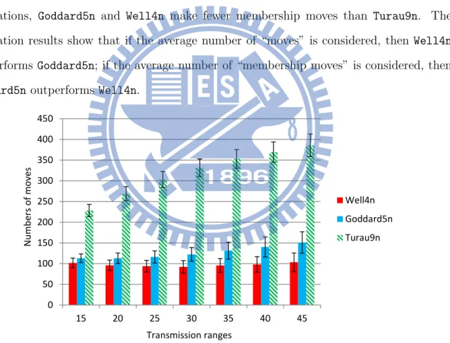
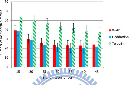
Figures 3.2 and 3.3 show the comparisons of the three algorithms. Figure 3.2 depicts the average number of “moves” with regard to the transmission ranges. In our simulations, Well4n always made fewer moves than Goddard5n and Turau9n. Figure 3.3 illustrates the average number of “membership moves” in terms of the transmission ranges. In our simulations, Goddard5n and Well4n make fewer membership moves than Turau9n. The simulation results show that if the average number of “moves” is considered, then Well4n outperforms Goddard5n; if the average number of “membership moves” is considered, then Goddard5n outperforms Well4n.

Transmission ranges N u mb er s o f mo v es 0 50 100 150 200 250 300 350 400 450 15 20 25 30 35 40 45 Well4n Goddard5n Turau9n

Figure 3.2: The average number of moves made by Well4n, Goddard5n, and Turau9n with regard to the transmission ranges, where the vertical line segments denote the standard deviations.

Before ending this section, we would like to point out an error in the modiﬁed Turau9n, which is called modiﬁed AMDS in [75]. Turau claimed (in page 93 in [75]) that rule 4 can

分散式系統之自我穩定極小控制集演算法與凱氏圖之正負號星控制數

國 立 交 通 大 學

應 用 數 學 系

博 士 論 文

分散式系統之自我穩定極小控制集演算法

與凱氏圖之正負號星控制數

Self-stabilizing Minimal Dominating Set Algorithms of

Distributed Systems and the Signed Star Domination

Number of Cayley Graphs

研 究 生：邱鈺傑

指導教授：陳秋媛

分散式系統之自我穩定極小控制集演算法

與凱氏圖之正負號星控制數

Self-stabilizing Minimal Dominating Set Algorithms of

Distributed Systems and the Signed Star Domination

Number of Cayley Graphs

研 究 生：邱鈺傑 Student: Well Y. Chiu

指導教授：陳秋媛 Advisor: Chiuyuan Chen

國 立 交 通 大 學

應 用 數 學 系

博 士 論 文

A Dissertation

Submitted to Department of Applied Mathematics

College of Science

National Chiao Tung University

in Partial Fulﬁllment of the Requirements

for the Degree of

Doctor of Philosophy

in

Applied Mathematics

July 2014

Hsinchu, Taiwan, Republic of China

摘要

圖論的控制集問題的研究始於 1960 年代。一個分散式系統 (例

如：一個隨意網路) 可以用一個無向簡單圖 G = (V, E) 來表

示，其中 V 表示點集，而 E 表示點跟點之間的聯結關係。圖

G

的點集 V 的子集合 D 被稱為是控制集，若此子集 D 具有

性質：V 中的任一元素 v 屬於 D 或與 D 中的元素相鄰。如果

一個控制集不真包含另一控制集，則稱其為極小控制集 (簡記

為 MDS)。極小控制集在無線網路中的應用之一是使所需的資

源中心保持為較少數目。

自我穩定是一個可用於設計分散式系統容忍暫時性錯誤的一個

概念，並且是在 1974 年由 Dijkstra 提出。一個分散式系統是

自我穩定的，如果它滿足：不論初始組態為何，系統總是能保

證在有限時間內達到一個合法的 (正確的) 組態。此處所稱的

系統組態是由系統中所有節點的狀態所組成。一個自我穩定演

算法由一些規則所組成，每個規則都有其觸發條件及其對應動

作，該動作能通過更新節點的變數來改變節點的狀態。每執行

一個規則稱為是一步。本論文所提出的演算法的效能皆是以執

行總步數來計算。自我穩定演算法有許多不同的執行模式，且

執行模式是以排程器的概念來呈現。排程器分為公平的及不公

平的兩種。眾所皆知，不公平的分散式排程器比其他類型的排

程器更貼近實際使用狀況。

令 n 表示給定的分散式系統的節點數。在 2007 年，Turau 對

於 MDS 問題，提出了不公平的分散式排程器下的第一個線性

時間的自我穩定演算法，此演算法在最多 9n 步之後穩定。在

2008 年，Goddard 等人改進了上述演算法並做到最多 5n 步。

我們將在本論文中提出一個採用不公平分散式排程器下最多

4n

步的自我穩定 MDS 演算法。

理想中，MDS 演算法是希望能做到 MDS-靜止的，亦即，若分

散式系統的初始組態已經是一個 MDS，則演算法將不執行任

何動作。值得注意的是，在正常模式中，一個節點只能取得其

一步內鄰居的資訊，我們稱這些資訊為 1 步資訊。不幸的是，

在本論文中，我們將證明：1 步資訊不足以建立一個 MDS-靜

止的演算法。在本論文中，我們將討論此一問題，並針對自我

穩定 MDS 演算法提出一個新的性能評量，稱為穩定性。我們

推廣這部份的結果至其他自我穩定演算法，並將自我穩定演算

法分類為四個層次。特別的是，我們將證明：在 2 步資訊模式

下，可建構出自我穩定 MDS-靜止的演算法，且其穩定時間之

上界為 2n 步。

在 2005 年，Xu 提出了圖的帶正負號星控制集的概念，在 2007

年，Wang 給出了完全圖的帶正負號控制數，詳細定義請參見

本論文的第五章。在 2010 年，Atapour 等人定義了帶正負號

星控制劃分數，並利用完全圖具有可完全 1-因子分解或可完全

漢米爾頓圈分解的性質，計算出完全圖的帶正負號星控制劃分

數。在 2012 年，我與印度學者 Chelvam 等人合作，定義了有

向圖的帶正負號星控制數，給出了全部有向凱式圖的帶正負號

星控制數，與無向凱式圖的帶正負號星控制數的部份結果，並

國立交通大學

應用數學系

博士論文

研究生：邱鈺傑

研究生：邱鈺傑 Student: Well Y. Chiu

國立交通大學

應用數學系

博士論文