行政院國家科學委員會專題研究計畫 成果報告
常數彈性變異數過程下考量破產程序的資本結構模型與實
證分析
研究成果報告(精簡版)
計 畫 類 別 : 個別型 計 畫 編 號 : NSC 99-2410-H-009-025- 執 行 期 間 : 99 年 08 月 01 日至 100 年 07 月 31 日 執 行 單 位 : 國立交通大學財務金融研究所 計 畫 主 持 人 : 李漢星 計畫參與人員: 碩士班研究生-兼任助理人員:黃鈺紜 碩士班研究生-兼任助理人員:劉猛綜 碩士班研究生-兼任助理人員:林哲銘 公 開 資 訊 : 本計畫可公開查詢中 華 民 國 100 年 10 月 31 日
中文摘要: 本文延伸 Francois and Morellec (2004)與 Broadie and Kaya (2007)的研究,使用二元樹模型,評價具到期日與第十一章破 產法規架構下之公司債。為了使模型更有彈性,並更貼近實 際,我們允許標的資產價格波動度變動,亦即發展一個常數彈 性變異數(CEV)過程下,考量破產程序的資本結構模型。本研 究數值分析結果指出,當重整的期限越長,或是 CEV 過程的彈 性係數越小時,公司債價值越低。 英文摘要:
行政院國家科學委員會補助專題研究計畫
■
成 果 報 告
□期中進度報告
常數彈性變異數過程下考量破產程序的資本結構模型與實證
分析
計畫類別:■ 個別型計畫 □ 整合型計畫
計畫編號:NSC 99-2410-H-009-025-
執行期間:2010 年 08 月 01 日至 2011 年 07 月 31 日
計畫主持人: 李漢星
共同主持人:
計畫參與人員:黃鈺紜、劉猛綜、林哲銘
成果報告類型(依經費核定清單規定繳交):■精簡報告 □完整報告
本成果報告包括以下應繳交之附件:
□赴國外出差或研習心得報告一份
□赴大陸地區出差或研習心得報告一份
□出席國際學術會議心得報告及發表之論文各一份
□國際合作研究計畫國外研究報告書一份
處理方式:除產學合作研究計畫、提升產業技術及人才培育研究計畫、
列管計畫及下列情形者外,得立即公開查詢
□涉及專利或其他智慧財產權,□一年□二年後可公開查詢
執行單位: 國立交通大學財務金融研究所
中 華 民 國 100 年 10 月 31 日
附件一1. Introduction
The structural credit risk modeling or defaultable claim modeling is pioneered by the
seminal paper by Black and Scholes (1973) in which corporate liabilities can be viewed as a
covered call — own the asset but short a call option. Later on, Merton (1974) rigorously
elaborates the pricing of corporate debt. This Black-Scholes-Merton approach of modeling
default claims is named structural approach since the model explicitly ties default risk to the firm
value process and its capital structure. In the capital structure models, the most notable
developments are the works by Leland (1994) and Leland and Toft (1996). These two studies
extend the endogenous default approach by Black and Cox (1976) to include the tax shield of
debt and bankruptcy costs, and explicitly analyze the static tradeoff theory of capital structure.
Various important issues including the endogenous default boundary, leverage ratio, debt value,
debt capacity, yield spread, and even potential agency costs are discussed in detail. Leland (1994)
and Leland and Toft (1996) provide closed-form expressions of corporate securities as well as
comparative statics. Their methodology and stationary debt structures are widely adopted in the
literature. In addition, these two models have been served as benchmark models in the optimal
capital structure literature.
According to the Leland (1994) and Leland and Toft (1996) models, bankruptcy is triggered
when shareholders find that running the company is no longer profitable, even when the cash
flows produced by the assets may still capable of servicing the debt. Therefore, bankruptcy is
determined endogenously rather than by a certain level of net asset or cash flow constraint While
the Leland (1994) and the Leland and Toft (1996) models provide some insights of the capital
structure issues, their predicted optimal leverage and yield spreads seem not to be consistent with
historical average. Consequently, the more recent studies introduce additional realistic features in
order to meliorate the model-predicted leverage and yield spreads. A line of research has been
advanced by Fan and Sundaresan (2000) who introduce a bargaining game between shareholders
and debtholder to determine the optimal bankruptcy boundary. Later on, Francois and Morellec
bankruptcy decisions.
.The U.S. bankruptcy code, which includes a liquidation process (Chapter 7) and
reorganization process (Chapter 11), is used to deal with the issues of a firm facing financial
distress. Contractual agreements and bankruptcy laws may cause different outcome when the firm
fails to make debt payments and declares bankruptcy. For example, bankruptcy may lead to
liquidation under Chapter 7, reorganization under Chapter 11, or the debt renegotiation between
debt holders and equity holders. Due to the reorganization period granted by the bankruptcy code
of Chapter 11, one can therefore regard the corporate equity as a consecutive down-and-out
Parisian option, which permits a period of time the underlying asset can stay below the
bankruptcy boundary before liquidation.
On the other hand, in order to introduce realism into the possible movement of the firm
value, Hilberink and Rogers (2002) and Chen and Kou (2009) add jumps into the asset value
process, which implies that the asset value of the firm can suddenly drop drastically and causes a
default. Hence, default is not a predictable event any more, and the credit spread increases in the
short-term. However, stochastic volatility feature, another important and commonly adopted
assumption in option pricing, is still rare in structural modeling literature. It is also reasonable to
conjecture that the volatility of firm value process is not a constant through time. The firms value
volatility could be higher while the firm value is low (The well-known leverage effect in option
pricing).
However, in order to obtain closed-form solutions of corporate securities, researchers need to
impose some unrealistic assumptions to avoid time and path dependence, for example, the
stationary debt structure, as assumed by Leland (1994) and the Leland and Toft (1996). These
models usually price infinite maturity bonds or continuously rollover bonds although these bonds
are rarely used in practice, especially when firms are in financial distress. By contrast, for finite
maturity bonds, it is difficult to obtain analytical solutions in models of bankruptcy proceedings
that include grace periods since it introduces path dependency. To overcome the difficulties,
option pricing literature, into structural credit risk modeling. Therefore, in this study, we extend
the work by Broadie and Kaya (2007) to develop a capital structure model with the feature of
Chapter 11 bankruptcy proceedings under the CEV process.
The CEV model proposed by Cox (1975) and Cox and Ross (1976) is complex enough to
allow for changing volatility and simple enough to provide a closed form solution for options
with only two parameters. The CEV process has the advantage that the volatility of the
underlying asset is linked to the level of underlying asset, which is consistent with the empirical
observation that the underlying asset volatility tend to change as the underlying asset moves up
and down. Although the CEV model is not as general and flexible as the stochastic volatility
models, its simplicity may still be worth exploring since those generalized models are expensive
to implement, especially when one applies to a capital structural model with a more realistic and
complex setting of bankruptcy proceedings. When applied to structural models, especially in the
case of Chapter 11 modeling with path-dependency, high-dimensional lattice models are very
expensive. One distinguish feature of the CEV model as opposed to other stochastic volatility
models is that it requires only a two-dimensional lattice (Nelson and Ramaswamy (1990) and
Boyle and Tian (1999)) as the models under geometric Brownian motion assumption. Its
parsimonious setting accommodates the well-known leverage effect, the inverse relationship
between the level of the underlying primitive variable and its variance of return.
This study contributes to existing literature in applying the CEV process to structural credit
risk modeling, which has not yet been explored in literature. We extend the binomial lattice
method by Broadie and Kaya (2007) to develop a capital structure model, which incorporates
finite maturity as well as the feature of Chapter 11 bankruptcy proceedings. Our numerical results
also show that the value of risky debt can be substantially affected by these features we
considered – When the reorganization period is longer or the elasticity constantis smaller, the value of corporate risky debt will be lower. Moreover, as has been mentioned, this model
equipped with changing volatility feature can be implemented without too much extra
The remainder of this paper is organized as follows. Section 2 reviews literature. Section 3
describes our model and how to incorporate the CEV process, Chapter 11, and finite maturity
features by using the binomial lattice method. Section 4 presents the numerical results in detail
and illustrates the model implications. Section 5 summarizes and concludes our paper.
2. Literature Review
2.1 Modeling Bankruptcy Proceedings in Capital Structure Models
We summarize related literature in two of the most relevant fields, namely, modeling
bankruptcy proceedings in capital structure models, and the CEV process and option
pricing.
(I) Modeling bargaining between holders and equity holders – The Fan and Sundaresan Model (2000)
Fan and Sundaresan (2000) propose a game-theoretic setting which incorporates equity’s
ability to force concessions and varying bargaining powers to the debt holders and equity holders.
Two cases are discussed in their study when the firm’s asset value falls below a certain boundary:
Debt-equity swap and strategic debt service. In the case of debt-equity swap, the debtholders
exchange their claims for equity. In strategic debt service, borrowers stop making the contractual
coupon and start servicing debt strategically until the firm’s asst goes back above the boundary
again.
Some key assumptions under their framework include: (1) During the default period, the tax
benefits are lost. (2) Asset sales for dividend payments are prohibited. (3) The firm can be
liquidated only at a cost. The proportional cost is(0 1)and the fixed cost isK(K 0). Note that debt holders have strict absolute priority upon liquidation.
(4) The asset value of the firm follows the lognormal diffusion process
t VdB Vdt
q
dV ( ) (1)
firm’s cash payout ratio.
We present only the results of strategic debt service which will be further explored in our
study. If the equity and debt holders can reach an agreement of temporary coupon reduction when
the firm is under financial distress, the firm will not lose its potential future tax benefits. At the
trigger point for the strategic serviceV~S, both parties will bargain the total value of the firmv(V).
The driving force behind strategic behavior is the presence of proportional and fixed costs of
liquidation. The bargaining power of equity holder clearly depends on the liquidation
costVS K. Fan and Sundaresan (2000) endogenize both the reorganization boundary and the optimal sharing rule between equity and debt holders upon default.
The total value of the firm is
S S C S S C C V V when V V r C T V V V when V V r C T r C T V V v ~ , ~ ~ , ~ ) ( (2) where 2 2 2 2 2 5 . 0 5 . 0 r r r
For anyV V~S, Fan and Sundaresan set the optimal sharing rule between shareholders and debtholders as ) ( ~ ) ( ~ V v V E andD~(V)(1~)v(V). (3)
The Nash solution to the bargaining game can be characterized as
* 1 0 , ) 1 ( max ) ( ) ~ 1 ( 0 ) ( ~ max arg ~ K V V v V v , ) ( ) 1 ( min V v K V (4)wheredenotes bargaining power of shareholders.
contractual coupon and still permit shareholders to run the company. This results in deviations
from APR, in which the shareholders will get a bigger share and the debtholders will get a less
proportion of the firm. But both parties will be better off. Therefore, the concession of
debtholders is well explained under the Fan and Sundaresan’s framework. They then solve the
trigger point for strategic debt service (K=0 case) and the strategic service amount paid to debt
holdersS(V)(1)qV .
The Fan and Sundaresan model shows that debt renegotiation encourages early default and
increases credit spreads on corporate debt, given that shareholders can renegotiate in distress to
avoid inefficient and costly liquidation. It might be the interest of debt holders to forgive part of
the debt service payments if it can avoid the wasteful liquidations, which can be shared by the
two claimants. If shareholders have no bargaining power, no strategic debt service takes place and
the model converges to the Leland model. Furthermore, by introducing the possibility of
renegotiating the debt contract, the default can occur at positive equity value. This is in contrast
to the Leland’s (1994) model in that the default occurs when the equity value reaches zero as a
consequence of that issuing new equity is costless and the APR is respected.
(II) Modeling Chapter 11 Bankruptcy Proceedings – Francois and Morellec (2004)
Francois and Morellec (2004) extend the Fan and Sundaresan (2000) model to incorporate
the possibility of Chapter 11 filings. Under their setup, shareholders hold a Parisian down-and-out
option on the firm’s asset, i.e., shareholders have a residual claim on the cash flows generated by
the firm unless the value of these assets reaches the default threshold and remains below that
threshold for the exclusive period. It is generally acknowledged that there are two types of
defaulting firms: First, firms that are economically sound, but default only due to temporary
financial distress, and recover under Chapter 11. Second, firms that are economically unsound,
keep on losing value under Chapter 11, and eventually liquidated under Chapter 7. The modeling
philosophy comes from the empirical studies which show that most firms emerge from Chapter
Following the Nash bargaining game of Fan and Sundaresan’s approach1, Francois and
Morellec presume the firm renegotiates its debt obligations whenever the asset value falls below a
constant thresholdVB. However, a major difference from Fan and Sundaresan’s model is that
Francois and Morellec assume that a proportional costs are borne by the company during the renegotiation process. The costs of financial distress incurred by the firm filing Chapter 11 are
ignored in the prior research. Even though the costs implied by private workouts generally are
low, Chapter 11 filings are associated with large costs of financial distress that may affect
shareholder’s default decision. Note that Leland (1994) only allows liquidation while Fan and
Sundaresan (2000) only permit private workouts.
Francois and Morellec solve the endogenous default barrier by maximizing equity value, and
provide closed-form solutions for corporate debt and equity values. They find that the possibility
to renegotiate the debt contract has ambiguous impact on leverage choices and increases credit
spreads on corporate debt. The sharing rule of cash flows during bankruptcy has a large impact on
optimal leverage, while credit spread on corporate debt shows little sensitivity to the varying
bargaining power.
(III) Binomial Lattice Method for Modeling Chapter 11 Proceedings – Broadie and Kaya (2007)
Broadie and Kaya (2007) develop a binomial lattice method that can be used handle more
real but complex structural models such as the finite maturity case of Leland (1994) or the models
of Brodie, Chernov, and Sundaresan (2007). Broadie and Kaya (2007) assume that the firm’s
asset valueV of is independent of the capital structural choices and its evolution under the t risk-neutral measure Q as follows:
t t t dW dt q r V dV ( ) (5) 1
Note that the specification for the bargaining game within Francois and Morellec’s framework is slightly different from that of Fan and Sundaresan (2000). Francois and Morellec focus on Chapter 11 filings— court-supervised debt renegotiation in contrast to the private workouts by Fan and Sundaresan. Therefore, the automatic stay of assets prevents shareholders from liquidating the firm’s assets. Nevertheless, renegotiation plan requires each participant to receive a payoff that exceeds the liquidating value of its claims. As a result, bondholders’ payoff has to
whereW is a standard Brownian motion under Q, r is the constant risk-free rate, q is the payout t
ratio (or cash flow) of the firm, is the volatility of asset returns.
The instantaneous cash generated by the firm is denoted astandt qVt. They assume that the firm issues a bond that promises to pay coupons at a continuous constant rateC, until a
default event occurs. The coupon is paid from the cash flowtgenerated by the firm at time t. Equity holders receive the remaindert Cin the form of dividends. In the case that cash flows are not enough to make coupon payments, i.e.,C , )t (t C is the negative cash flow for equity holders. Broadie and Kaya (2007) show in their Proposition 1 that this is equivalent to
dilution of equity by the firm. More importantly, this treatment does not violate the limited
liability requirement.
They next apply the standard binomial branching process and compute the claim of equity
holders after debt issuance, E. The claim of the debt holders, D, and the total firm value, F, at
each node are given as follows:
) ) 1 ( ( u d t r E p pE e E (6) ) ) 1 ( ( u d t r D p pD e D (7) ) ) 1 ( ( u d t r F p pF e F (8)
The present value of equity ignoring the current coupon payment and the cash flow is
denoted as E~. If the difference between the coupon payment and the current cash flow is denoted
byC C , Broadie and Kaya (2007) show that
C E if C E C E if E ~ ~ ~ 0 (9)
This result indicates that one needs not go through tedious calculations of equity dilution at
each step even if the firm’s cash flow is not enough to cover the coupon payment.
2.2 Parisian Options
Under the setup of Francois and Morellec (2004), shareholders hold a Parisian down-and-out
option on the firm’s asset in the presence of Chapter 11 filings. Parisian option is a variant of
the activation of a Parisian option depends on the time spend above or below the barrier. For
example, a down-and-out option is void when the underlying spends more than a specified time
strictly below the barrier.
Parisian option can be valued by various methods. Chesney et al. (1997) use Laplace
inversion to compute Parisian option value. Avellaneda and Wu (1999) obtain a lattice scheme for
calculating the price and sensitivities of such options. Costabile (2002) provides a discrete time
algorithm to evaluate European Parisian options. Bernard et al. (2005) develop a new inverse
Laplace transform method that is quick and appropriate to the pricing problem. Costabile (2002)
provides a discrete time algorithm to evaluate European Parisian options with flat or exponential
barriers. His approach is based on a combinatorial tool for counting the number of paths that
remains below a barrier for a period strictly smaller than a pre-specified time interval.
In this paper, we use a variant of the lattice-based method, called the forward shooting grid
(FSG), which has been successfully applied to price path-dependent options. The FSG approach
was developed by Hull and White (1993) and Ritchken, Sankarasubramanian and Vijh (1993) for
the pricing of American- and European-style Asian and lookback options. The FSG approach uses
auxiliary state vector at each node on the lattice. The state vector can be used to capture the
path-dependent feature of the option contract, like grace period of the asset price. This feature is
closely related to the Chapter 11 bankruptcy code in the context of capital structure modeling.
2.3 The CEV Process and Option Pricing
An important issue in option pricing is to find a stock return distribution that allows
returns to stock and its volatility to be correlated with each other. There is considerable empirical
evidence that the returns to stocks are heteroscedastic and the volatility of stock returns changes
with stock price. A great deal of empirical evidence indicates that stock volatility is negatively
related to stock price, and it is so-called leverage effect first discussed by Black (1976). To
accommodate this leverage effect, the Constant Elasticity of Variance (CEV) model by Cox (1975)
and Cox and Ross (1976) relaxes the constant volatility assumptions of the Black-Scholes model
underlying asset. The rationale for an inverse relationship between the stock price and its
variance of return can be explained by some simple economic arguments. Researchers use both
financial and operating leverage arguments. A decline in a leveraged firm’s stock price may lead
to an increase in its debt-equity ratio, hence the riskiness of the stock increases. Even if a firm has
no debt, the decline of the stock price can make it more difficult for the firm to meet its fixed
costs and thus has effect to increase volatility.
The CEV model assumes the diffusion process for the stock is
dS SdtS/2dz, (10)
and the instantaneous variance of the percentage price change or return,2, follows deterministic relationship: ) 2 ( 2 2 ) , ( S t S (11)
where the elasticity of this variance with respect to the stock price equals.
If =2, prices are lognormally distributed and the variance of returns is constant, which is the same as the well-known Black-Scholes model. If <2, the stock price is inversely related to the volatility. Cox originally restricted0 2. Emanuel and MacBeth (1982) extended his analysis to the case 2and discuss its properties. However, Jackwerth and Rubinstein (2001) find that typical values of thecan fit market option prices well for post-crash period only when 0, and they called the model with 0unrestricted CEV model2. In their empirical study, the difference of pricing performance of restricted CEV model ( 0) and BS model is not significant.
When<2, the nondividend-paying CEV call pricing formula is as follows:
0 0 ) 1 | ( ) 2 1 1 | ( ) 2 1 1 | ( ) 1 | ( n r n n K G n S g Ke n K G n S g S C (12)When >2, the CEV call pricing formula is as follows:
2
The unrestricted CEV model is mathematically legitimate. However, there are some economic arguments
supporting on a restriction on the parameter. For example, it is inconceivable for the stock index to have a
significant probability of bankruptcy while this is likely with sufficiently negative. See the detail in Jackwerth and
(Eq 2.1.4)
0 0 ) 2 1 1 | ( ) 1 | ( 1 ) 1 | ( ) 2 1 1 | ( 1 n r n n K G n S g Ke n K G n S g S C (13) where 2 ) 2 ( 2 ) 2 ( ) 1 )( 2 ( 2 S e re S r r 2 ) 2 ( 2 ) 1 )( 2 ( 2 K e r K r ) ( ) | ( 1 m x e m x g m x is the gamma density function
x g y m dy m x G( | ) ( | )C is the call price; S, the stock price; , the time to maturity; r, the risk-free rate of interest; K, the strike price; andand , the parameters of the formula.
Schroder (1989) expressed the CEV call option pricing formula in terms of the noncentral
chi-square distribution: When <2, )) 2 ), 2 /( 2 2 ; 2 ( 1 ( ) 2 ), 2 /( 2 2 ; 2 ( y x e K Q x y Q S C rt t (14) When >2, )) 2 ), 2 /( 2 2 ; 2 ( 1 ( ) 2 ), 2 /( 2 2 ; 2 ( x y e K Q y x Q S C t rt (15) ) , ; (z v k
Q is a complementary noncentral chi-square distribution function with z , v , andkbeing the evaluation point of the integral, degree of freedom, and noncentrality, respectively,
where ) 1 )( 2 ( 2 ) 2 ( 2 r e r k (2 ) 2 r t e kS x 2 kK y
3. The model
This section presents the details of our capital structure model under the CEV process. We
first denote the asset value of the firm V and use it as the primitive variable. We assume that the t
asset value V is independent of the capital structure and other financial decisions. The diffusion t
process follows the constant elasticity of variance (CEV) of Cox and Ross (1976) under the
risk-neutral measure Q and it is given by
2 t t t t dV r q V dt V dW (16) where W is a standard Brownian motion under Q, q is the payout ratio of the firm, and t isthe volatility of asset returns. is a constant, know as the elasticity factor, and 0 . In 2 the case when , equation (1) reduces to geometric Brownian motion, and this implies that 2 geometric Brownian motion is a special case of the CEV process.
3.1 A binomial lattice under the CEV process
We construct a discrete approximation for the CEV process using the binomial method.
Nelson and Ramaswamy (1990) derived a binomial approximation of the stochastic process
described in (1) in which a “computationally simple binomial tree” is proposed in order to let the
number of nodes in the tree structure grows linearly with number of time intervals. We let
, y y t V .Applying Ito’s Lemma, the stochastic differential equation for y is
2 2 2 2 1 2 t t t t t y y y y dy r q V V dt V dW t V V V (17)In order to have a constant diffusion coefficient for the Y-process, we let
2 t y V V , (18) for some positive constant . Equation (3) is equal to
2 t y V V ,
1 2 2 1 t t y V (19) and for , the transformation is given by 2
ln t t y V Thus we can build up a computationally simple binomial tree to approximate the y -process. The
two-dimensional grid in the
t y, -space can be built as follows. The value y of the process at t time t, after one period at timet1, can rise to yt t or decrease toyt t . In this way, we can build up the value of the y -process as
2
j
t i t t
y y j i , t i , 0, ,n j 0, ,i
where yt i tj represents the value on the binomial tree under y -process at time t i t after j up steps and i down steps. Next, to build up a binomial tree with j V -process on the
two-dimensional grid in the
t V, space, we can use the inverse transformation of (19)
2 1 1 2 1 , if 0 0, otherwise. t t t y y V (20)Once we have constructed the binomial tree with V -process, we can define the probability of
each up step. First we define Vt i t j to be the greatest Vt i t j , j , making 0, ,i
1 0
r t j j
t i t
t i t
e V V , and Vt i t j to be the smallest Vt i t j , j , making 0, ,i
1 0
j r t j
t i t t i t
V e V . The probability with
t V, space makes an up steps is 1 1 if 0 0 otherwise j r t j t i t t i t j j j j t i t t i t t i t t i t e V V V p V V (21)
The probability of down steps is thus qtj i 1 t 1 ptj i 1 t. With the definition given above,
1
j
t i t
p represents a probability for the evolution of the value of underlying asset in the binomial
Next, we would like to compute the value of equity, debt and firm on the lattice. We denote
equity value as E , the value of the debt holder as D , and the total firm value by F . For simplicity,
we drop the indexes of the probabilityptj i 1 t hereafter. At current node, the present value of the
equity is given by
1
r t u d Ee pE p E (22) The values of D and F also can be calculated in the same way:
1
r t u d De pD p D (23)
1
r t u d F e pF p F (24) Assume that at the current node, the firm has to pay coupon payment C and firm’s cashflow ist. The present value of equity which do not consider current coupon payment and current firm cash flow is given by
1
r t
u d
E e pE p E (25)
We denote the difference between the coupon payment and firm cash flowC . When the C t
coupon payment is less than the firm cash flow, C is negative and it means that excess firm cash
flow over the coupon payment can be receive by equity holders. If C is positive, it means equity
holders should raise money by equity dilution. Broadie and Kaya (2007) have shown that equity
value at the current node is as follows:
0 if if E C E E C E C (26) This result indicates that one needs not go through tedious calculations of equity dilution at
each step even if the firm’s cash flow is not enough to cover the coupon payment.
3.2 Setup for the bankruptcy with grace period and bargaining
In the real world, the equity holders can liquidate the firm under Chapter 7 of the U.S.
bankruptcy code or renegotiate debt payments under Chapter 11. Under Chapter 11, the
bankruptcy court allows the firm to restructure its debt during a certain grace period. Chapter 11
bankruptcy under Chapter 11 when it is in financial distress, and it spends some time as a
bankruptcy firm which does not make full coupon payment, and then recover to become a healthy
firm.
Following Francois and Morellec (2004), we assume that equity holders decide to declare
bankruptcy at a certain level of the firm asset valueVB, and a grace period G is granted by bankruptcy court. If the firm does not come out from bankruptcy at the end of the grace period,
the firm is liquidated. When the firm is in bankruptcy, distress cost reduces the net firm cash flow. When the firm asset value is under the default boundaryVB, debt is serviced strategically. At the time bankruptcy is declared, the debt service is determined by the bargaining game between
debt holders and equity holders.
We follow the setting of Fan and Sundaresan (2000) to determine the debt service using a
Nash bargaining game. Denote the proportional liquidation cost as . If the firm is liquidated at the bankruptcy point, the debt holders receive
1
VB and equity holders receive nothing. If the firm is not liquidated, firm asset value will beB
V
F , and will be share between debt holders and
equity holders.
We assume the bargaining power of the equity holders is and the bargaining power of debt holders is1 . If we denote the sharing rule at the bankruptcy point as , the incremental value gained by equity holders is
B
V
F
and the incremental value gained by debt holders
is
1
1
B V B F V .The optimal sharing rule is
1
* arg max 1 1 B B B V V V F F F (27)and its solution is
* 1 1 B B V V F (28) As a result, at the bankruptcy point, the value of the claim of the equity holders is
* 1 B B V V B F F V (29)and the value of the claim of the debt holders is
*
1 1 1 1 B B V V B B F F V V (30)The bargaining game determines the value of equity and debt at the bankruptcy point through
equation (29) and (30). Thus we do not need to know how the debt is serviced when firm is in
bankruptcy, just need to know the total firm valueF . B
3.3 Binomial lattice computations
We use the binomial lattice under the CEV process as described in section 3.1. If the bond is
a consol bond, the bankruptcy boundary will be constant and time independent. However, if the
bond has finite maturity, the bankruptcy boundary will be time dependent. First we price infinite
maturity debt. The bankruptcy boundaryVBis assumed to be known at each time step in the lattice.
The optimal level ofVBcan be solve numerically later. We assume that the default boundary V B
fits with the level of nodes on the lattice. If it is not on the lattice, we use the first node level that
is higher than V to approximateB V . We assume firm has issued a consol bond with coupon B
payment C. The effective tax rate is and all interest payments are tax deductible. In the
binomial lattice, due to discrete time steps, the total firm cash flow at a certain node with asset
value is given by:
q t
t V et Vt
(31)
Following Broadie and Kaya (2007), according to the position of nodes on lattice, we next
perform the binomial lattice computation among the following three conditions.
Condition (i): The firm is in a healthy condition ( Nodes withV VB)
The firm is in a healthy state in these nodes, the coupon payments are paid either by firm
cash flow or equity dilution if firm cash flow is not enough to pay the coupon payments. The
effective tax rate is . Equity, debt, and firm value can update as follows:
If 1 : 1 , 1 , 1 . t t r t u d r t t u d E C t E E C t D C t e pD p D F e pF p F C t (32)
If 1 : 0, 1 , 1 . t t t t t E C t E D V F V where E is given in (10) and t is given in (16).
Condition (ii): The firm is in bankruptcy (Nodes with V VB)
The firm is in bankruptcy. The debt is serviced strategically and we do not know how the
firm cash flow is shared between debt holders and equity holders. We can use equation (29) and
(30) to determine the value of debt and equity at the bankruptcy point, so we only need to track of
the firm value F when the firm is in bankruptcy. In addition, there are no tax benefits while the
firm is in bankruptcy.
The total time spent below the default boundary V needs to be recorded. Let g record B
the length of time the firm spends in bankruptcy. Because we are working on the binomial lattice,
g can only take discrete values. Let g denote the maximum number of time steps that the firm
can spend in bankruptcy. We haveg G t
, whereGis the grace period. Assume g is an integer, and then g will be the value in
0,1,,g1,g
. For a given node and a given g , there exists three possibilities in the next time steps. First, the firm comes out of bankruptcy next timestep. Second, if g in the current node, and g 1 V VB in the next time step, then the grace period will be in expiration and the firm will be liquidated. Finally, the firm can still be in
bankruptcy without expired grace period in the next time step. Thus the value of g will be one
higher than the current node. For each node, we need to keep track of the firm value in every
possible state of g . Thus, F i
will represent the firm value at the current node when g . We ican update the firm value as follows:
1 1 1 for 1, , 1 1 for r t t u d t t e pF i p F i i g F i V i g (33) where q t t V et Vt (34)and t represents the distress cost adjusted cash flow of the firm.
Condition (iii): The last healthy state before the firm into bankruptcy or the first state after the
firm out of bankruptcy — (Nodes with V VB)
This node is the last healthy state before firm goes into bankruptcy or the first healthy state
the firm just comes out from bankruptcy. The equity and debt values can be calculated using
equation (29) and (30) after firm value is computed. We update equity, debt, and firm values as
follows:
0 1 1 , 1 1 for 1, , , 0 1 , 1 0 1 1 . r t t u d r t t u d B B B F e pF p F F i e pF p F i g E F V D F V V (35)
0F represents the value of the firm at the bankruptcy boundary V that has never been in B
bankruptcy, and it is the value for the node reaching V from above. TheB F i
is the value of the firm at the bankruptcy boundary V just coming out from bankruptcy. As the result, B F i
takes into account the distress cost, while F
0 does not.3.4 Pricing finite maturity debt
We can use the procedure described in Section 3.3 for pricing finite maturity bond with
coupon C, face value P and maturity T .At maturity, the face value and the coupon payment
should be paid; otherwise the firm will be liquidated. If the firm is still under the bankruptcy
boundary V when the bond matures, the firm will be liquidated. The terminal values will be B
calculated as follows: 1. Nodes with V VB
If 1 : 1 If 1 : 0 T T T T T T T T V C t P E V C t P D C t P F V C t V C t P E
1 1 T T T T D V F V (36)2. Nodes with V VB
1
T T
for 1, , F i V i (37) g 3. Nodes with V VB
If 1 : 1 0 T T T T T T T V C t P E V C t P D C t P F V C t F i V
for 1, , If 1 : 0 1 0 1 T T T T T T T C t i g V C t P E D V F V
F i 1 VT T for i 1, ,g (38)Optimal bankruptcy boundary
We assume that V is a vector that contains the bankruptcy boundary for each time steps. B
The optimal V in the finite maturity setting will not be constant, but will be time dependent B
since the remaining value of the bond is changing over time. Therefore, we assume a functional
form for the bankruptcy boundary and let the equity holders choose a parameter of that function
to maximize the equity value. Following Broadie and Kaya (2007), we use a linear function of the
riskless bond price.
t
B t
V P (39)
t B
V is the bankruptcy boundary at an intermediate time t , P is the riskless bond price at time t
t , and is a positive number that is time independent. Also, if V is not on the lattice, we use Bt
4. Numerical Result 4.1 Numerical method
4.1.1 The FSG (Forward Shooting Grid) approach
We have already described the binomial lattice computation under the CEV process in
section 3. The most crucial and time consuming part is to deal with the path-dependent feature of
the grace period. In this paper, we adopt the Forward Shooting Grid (FSG) approach developed
by Hull and White (1993) to cope with nodes which are under the bankruptcy boundary. Let
,g k j denote the grid function. The binomial tree of the FSG algorithm can be represented by
1, ;
u , 1;
, 1
u , 1;
, 1
r t V m j k p V m j g k j p V m j g k j e (40)
, 1
j B x V g k j k 1 (41)Note that before we move to next time step, it is necessary to compute V m j k
, ;
for all indexk for k g 1, g2, , 0. In order to shorten the computation time and enhance efficiency, we do not compute k in all nodes. We only need to compute the nodes which are under the
bankruptcy boundary. In addition, it is also not necessary to compute V of various k for the
nodes which are below the bankruptcy boundary for more than g levels. This is because the
asset value of the firm can by no means go back to the level of bankruptcy boundary within grace
period.
4.1.2 Determination of optimal bankruptcy boundary
The optimal bankruptcy boundary must be chosen to maximize the equity value numerically.
In the case of infinite maturity debt, we choose an arbitrary bankruptcy boundary that is lower
than optimal boundary. And next we start to increase the boundary on the lattice and reprice the
equity value. The equity value first increases and then starts to decrease after it reaches the
maximum value when we move the boundary up on the boundary. Therefore, we stop moving the
boundary when the equity value starts to decrease. As a result, we can obtain the discrete
observation points and fit a cubic spline interpolation to approximate the exact functional form
maturity debt case, under the assumption of t
B t
V P, equity holders will choose a to
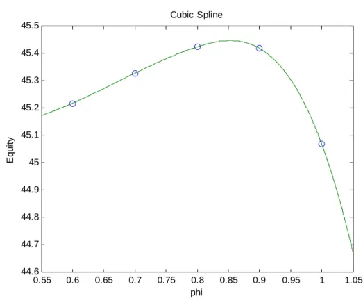
maximize the equity value. Similar to the case of infinite maturity debt, we choose arbitrary s and reprice the equity values. We then need to search for the appropriate and fit a cubic spline interpolation for the maximum equity value. Figure 1 illustrates the cubic spline interpolation to
find the equity maximizing boundary, VBt Pt, of finite maturity debt case.
Figure 1 Illustration of Cubic Spline Interpolation for Equity
The model parameters are V0 100, 20%, 3, 60, 5%, 3%, 50%, C P r q =1%, 25%, 50%, G 1, 1, T 5 t 0.005 years equity is 45.4476 0.55 0.6 0.65 0.7 0.75 0.8 0.85 0.9 0.95 1 1.05 44.6 44.7 44.8 44.9 45 45.1 45.2 45.3 45.4 45.5 phi Eq u it y Cubic Spline
4.1.3 Convergence of the binomial lattice method
To decide the appropriate number of time steps in our numerical study, the convergence of
lattice approach must be analyzed. Therefore, we compute the equity and debt values with 5000
time steps and set them as the true values. Then we analyze our pricing results by comparing the
values obtained from the lattice approach with the “true value” describe above. Figure 2 and
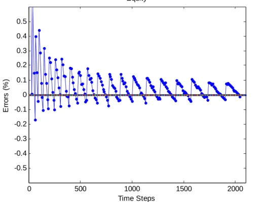
Figure 3 show, under and1 0.5, respectively, the convergence of equity and debt pricing errors as the number of time steps increases. The oscillation of pricing errors is due to the relative
determined endogenously by maximizing equity value, there is no way to force the bankruptcy
boundary to be laid on the lattice node to solve the oscillating behavior of the errors. Nonetheless,
one can observe that the size of pricing errors is relatively small when we use more than 1000
time steps. The largest error is less than 0.2% of the true value, and thus we will uset=0.005 (=5/1000) to perform the numerical study in the later section.
Figure 2. Convergence of Equity and Debt Errors (β=1)
The model parameters are V0 100, 20%, 3, 60, 5%, 3%, 50%, C P r q =1%, 25%, 50%, G 1, 1, T 5
. The true value of equity is 45.4671, and the
true value of debt is 55.0929.
0 500 1000 1500 2000 -0.5 -0.4 -0.3 -0.2 -0.1 0 0.1 0.2 0.3 0.4 0.5 Time Steps E rrors ( % ) Equity
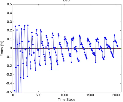
0 500 1000 1500 2000 -0.5 -0.4 -0.3 -0.2 -0.1 0 0.1 0.2 0.3 0.4 0.5 Time Steps E rro rs (% ) Debt
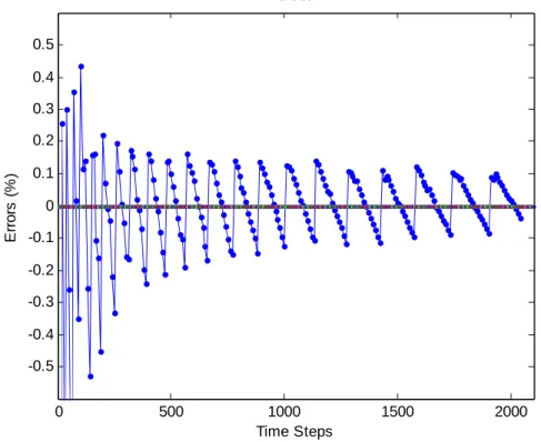
Figure 3. Convergence of Equity and Debt Errors (β=0.5)
The model parameters areV0 100, 20%, 3, 60, 5%, 3%, 50%, C P r q =1%, 25%, 50%, G 1, 0.5, T 5
. The true value of equity is 45.8437, and
the true value of debt is 54.9405.
0 500 1000 1500 2000 -0.5 -0.4 -0.3 -0.2 -0.1 0 0.1 0.2 0.3 0.4 0.5 Time Steps E rrors ( % ) Equity
0 500 1000 1500 2000 -0.5 -0.4 -0.3 -0.2 -0.1 0 0.1 0.2 0.3 0.4 0.5 Time Steps E rro rs (% ) Debt
4.2 Application and Analysis: Numerical Example
In this section, we first investigate the debt prices and the yield spreads of coupon bond with
finite maturity under various elasticity parameter of the CEV process, and next extend the analysis to the effect of different grace periods. We are aware of that the length of the granted
grace period in the Chapter 11 setting may have different impact on bonds with different maturity.
Therefore, we first set G=0 to examine the effect of maturity on debt value and yield spreads in
Figure 4. It is apparent that as the debt maturity increases, the price of the finite maturity coupon
bond converged to the price of the consol bond.
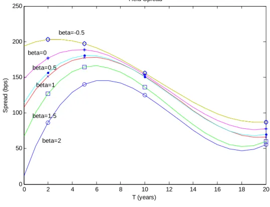
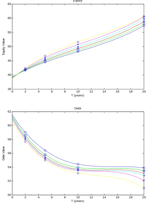
Figure 4 presents relationship between debt maturities and yield spread, equity value, and
debt value. The yield spread is defined as Credit Spreads=C/D-r , where r is a risk-free rate.
Consistent with the results of Leland and Toft (1996), under moderate leverage (V=100 and
P=60), the yield spread first rises with the increase of debt maturity until it reaches the peak for
around 5 to 6 years to maturity. The yield spreads then decrease at a decreasing rate as maturities
prolonged. Since a company under financial distress may not easily issue new debts, it is crucial
that term structure of yield spread in our study agrees with prior literature without having to have
In addition, the yield spreads are negatively related to the elasticity parameter of the CEV process. This is in line with the fact that the value of equity increases and the value of the debt
decreases as the decreases. The results are reasonable because the decrease in is associated with the rise of asset volatility. Therefore, equity, which can be viewed as a call option
on asset value3, increases its value. In contrast, debt holders who expect the firm to have steady
cash flow may suffer from the higher volatility caused by the lower.
Figure 4. Effect of Maturity on Yield Spreads, Equity, and Debt for a Coupon Bond for
Various
The model parameters areV0 100, 20%, 3, 60, 5%, 3%, 50%, C P r q =1%, 25%, 50%, G=0
. The time increment in the lattice is t 0.005 years.
0 2 4 6 8 10 12 14 16 18 20 0 50 100 150 200 250 T (years) S p re ad (b ps ) Yield Spread beta=2 beta=1.5 beta=-0.5 beta=0 beta=0.5 beta=1 3
Note that Leland and Toft (1996) indicated that equity in the capital structure model is not precisely analogous to an ordinary call option for several reasons: First, default may occur at any time but not only at debt maturity. Second, the bankruptcy boundary may vary with the risk of the firm's activities. Last and most importantly, the existence of tax benefits and their potential loss in bankruptcy imply that debt and equity holders do not split a claim whose value depends only on the underlying asset value.
0 2 4 6 8 10 12 14 16 18 20 35 40 45 50 55 60 65 T (years) E qui ty V a lu e Equity 0 2 4 6 8 10 12 14 16 18 20 50 52 54 56 58 60 62 T (years) D ebt V a lu e Debt
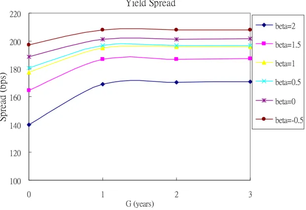
Figure 5 extends the analysis to the cases in the presence of grace period. Similar to the
previous results without grace period, when the of the CEV process decreases, the value of the equity increases and the value of the debt decreases. The reason is the same as before since
the volatility comes into play. Furthermore, it appears that as the grace period increases, the
equity value and yield spread increase at a decreasing rate and eventually converge to a certain
level. By contrast, debt value goes down as grace period prolonged. This is because the existence
of the grace period can benefit equity holders via reorganization while debt holders could not
case of bankruptcy, the firm is liquidated immediately and equity holders may receive nothing.
But if there is grace period for equity holders, equity holders can wait for firm recovery from
financial distress, not just only residual value after liquidation. More importantly, as indicated by
Francois and Morellec (2004), Chapter 11 filings involves potential debt service reduction and
lead to higher leverage ratio and hence higher yield spread.
Figure 5. Effect of Grace Period on Equity, Debt and Yield Spread
for a Coupon Bond with Various
The model parameters areV0 100, 20%, 3, 60, 5%, 3%, 50%, C P r q
=1%, 25%, 50%, T 5
The time increment in the lattice is
0.005 t years
Yield Spread
100 120 140 160 180 200 220 0 1 2 3 G (years)S
pr
ea
d
(
bps
)
beta=2 beta=1.5 beta=1 beta=0.5 beta=0 beta=-0.5Equity T=5 43 43.5 44 44.5 45 45.5 46 46.5 47 47.5 0 1 2 3 G (years) E qu ity V al ue beta=2 beta=1.5 beta=1 beta=0.5 beta=0 beta=-0.5 Debt T=5 53.5 54 54.5 55 55.5 56 56.5 57 0 1 G (years) 2 3 D ebt V al ue beta=2 beta=1.5 beta=1 beta=0.5 beta=0 beta=-0.5 5. Conclusion
In this paper, we introduce constant elasticity of variance (CEV) process into the popular
structural modeling framework of capital structure analysis. The CEV process allows the asset
volatility to change with the current level of asset value, and thus give the risky corporate debt
pricing model a more realistic touch. We extend the work by Francois and Morellec (2004) and
as well as the feature of Chapter 11 bankruptcy proceedings. While evaluating a single corporate
debt with finite maturity or complex bankruptcy proceedings, no analytical solution is available
and one needs to resort to numerical methods. Therefore, we adopt a lattice approach to price
risky corporate debt and generate results that are consistent with the limited liability of equity
principle. Furthermore, our study can be beneficial to corporate debt pricing model as well. While
many existing models use infinite maturity bonds to obtain a close-form solution, our method can
be used to price finite maturity debt.
In general, our numerical results for finite maturity debt are consistent with those of
previous literature. We first analyze the term structure of yield spreads for finite maturity debt
and leave out the Chapter 11 bankruptcy code. We find that under moderate leverage yield
spreads first rise up and then drop with the increase of debt maturity at a decreasing rate to a
certain stable level. Under different grace periods in Chapter 11 bankruptcy proceedings, the
equity value increases and the debt value decreases when the grace period prolonged. The results
are as expected because increasing in grace period is the extra benefit for equity holders while it
could potentially hurt debtholders. Furthermore, we also examine the effect of parameterof the CEV process. It is apparent that the decrease of under the CEV process, implying higher volatility, leads to a lower debt value, a higher yield spreads, and a higher equity value.
The future work of our study could be adding empirical investigation to examine the model
implications: Whether or not the low-asset-value firm indeed has a lower (high volatility)? Whether the grace period of Chapter 11 bankruptcy proceeds is positively associated with yield
spread and equity value? In addition to empirical aspects, improving the efficiency of the
numerical approach to shorten the computing time should be crucial for applying our model in
References
Avellaneda, M., and L. Wu, 1999, “Pricing Parisian-style options with a lattice method,”
International Journal of Theoretical and Applied Finance 2, 1–16.
Bernard, C., O.L. Courtois, and F. Quittard-Pinon. 2005, “A new procedure for pricing Parisian options,” Journal of Derivatives 12, no. 4: 45–53.
Black, F. and J. C. Cox, 1976, “Valuing Corporate Securities: Some Effects of Bond Indenture Provisions,” Journal of Finance 31, 351-367.
Black, F. and M. Scholes, 1973, “The Pricing of Options and Corporate Liabilities,” Journal of
Political Economy 81, 637-654.
Black, F., 1976 “Studies of Stock Price Volatility Changes,” Proceedings of the 1976 American
Statistical Association, Business and Economics Statistics Section, 177-181.
Boyle, P. P., and Y. Tian, 1999, “Pricing Lookback and Barrier Options under the CEV Process,“ Journal of Financial and Quantitative Analysis 34, No. 2, June, 241-264. (Correction: Boyle, P., Y. Tian, and J. Imai. Look-back options under the CEV process: A correction. JFQA website at http://depts.washington.edu/jfqa/hold/342BoyleCrx1.pdf.)
Broadie, M. and O. Kaya., 2007, “A Binomial Lattice Method for Pricing Corporate Debt and Modeling Chapter 11 Proceedings,” Journal of Financial and Quantitative Analysis 42, 279–312.
Broadie, M., Chernov, M., and S. Sundaresan, 2007, “Optimal Debt and Equity Values in the Presence of Chapter 7 and Chapter 11,” Journal of Finance 62, 1341-1377.
Chen, Nan and S. G. Kou, 2009, "Credit Spreads, Optimal Capital Structure, and Implied Volatility with Endogenous Default and Jump Risk," Mathematical Finance, Vol. 19 (3), 343–378.
Chesney, M., M. Jeanblanc-Picqu´e, and M. Yor, 1997, “Brownian excursion and Parisian barrier options,” Advances in Applied Probability 29, 165–184.
Cox, J. C., 1975, “Notes on Option Pricing I: Constant Elasticity of Diffusions,” Unpublished draft, Standford University, September.
Cox, J. C., and S. Ross, 1976, The valuation of options for alternative stochastic processes,
Journal of Financial Economics 3, 145-166.
Emanuel, D. C. and J. D. MacBeth, 1982, “Further Results on the Constant Elasticity of Variance Call Option Pricing Model,” Journal of Financial and Quantitative Analysis 17, 533-554.
Fan H. and S. Sundaresan, 2000, “Debt Valuation, Renegotiations and Optimal Dividend Policy,”
Review of Financial Studies 13, 1057-1099.
Francois, P., and E. Morellec, 2004, “Capital Structure and Asset Prices: Some Effects of Bankruptcy Procedures,” Journal of Business 77, 387-411.
Hilberink, B. and L. C. G. Rogers, 2002, “Optimal Capital Structure and Endogenous Default,”
Financial and Stochastics 6, 237-263.
Leland, H. E. and K. B. Toft, 1996, “Optimal Capital Structure, Endogenous Bankruptcy, and the Term Structure of Credit Spreads,” Journal of Finance 51, 987-1019.
Leland, H. E., 1994, Corporate debt value, bond covenants, and optimal capital structure, Journal
of Finance 49, 1213-1252.
Merton, R. C., 1974, “On the Pricing of Corporate Debt: the Risk Structure of Interest Rates,”
Journal of Finance 28, 449-470.
Nelson, D. B. and K. Ramaswamy, 1990, “Simple Binomial Processes as Diffusion Approximations in Financial Models,” Review of Financial Studies 3, 393-430.
Ritchken, P, L. Sankarasubramanian and A. M. Vijh, 1993, “The valuation of path dependent contracts on the average,” Management Science, 39, 10, 1202-1213.
Schroder, M., 1989, “Computing the Constant Elasticity of Variance Option Pricing Formula,”
國科會補助計畫衍生研發成果推廣資料表
日期:2011/10/29國科會補助計畫
計畫名稱: 常數彈性變異數過程下考量破產程序的資本結構模型與實證分析 計畫主持人: 李漢星 計畫編號: 99-2410-H-009-025- 學門領域: 財務無研發成果推廣資料
99 年度專題研究計畫研究成果彙整表
計畫主持人:李漢星 計畫編號: 99-2410-H-009-025-計畫名稱:常數彈性變異數過程下考量破產程序的資本結構模型與實證分析 量化 成果項目 實際已達成 數(被接受 或已發表) 預期總達成 數(含實際已 達成數) 本計畫實 際貢獻百 分比 單位 備 註 ( 質 化 說 明:如 數 個 計 畫 共 同 成 果、成 果 列 為 該 期 刊 之 封 面 故 事 ... 等) 期刊論文 0 1 100% 研究報告/技術報告 0 0 100% 研討會論文 0 0 100% 篇 論文著作 專書 0 0 100% 申請中件數 0 0 100% 專利 已獲得件數 0 0 100% 件 件數 0 0 100% 件 技術移轉 權利金 0 0 100% 千元 碩士生 3 3 100% 博士生 0 0 100% 博士後研究員 0 0 100% 國內 參與計畫人力 (本國籍) 專任助理 0 0 100% 人次 期刊論文 0 0 100% 研究報告/技術報告 0 0 100% 研討會論文 0 0 100% 篇 論文著作 專書 0 0 100% 章/本 申請中件數 0 0 100% 專利 已獲得件數 0 0 100% 件 件數 0 0 100% 件 技術移轉 權利金 0 0 100% 千元 碩士生 0 0 100% 博士生 0 0 100% 博士後研究員 0 0 100% 國外 參與計畫人力 (外國籍) 專任助理 0 0 100% 人次其他成果