基於區域可變式視窗大小和適應性權重的視差估計演算法

(1)

國立交通大學

資訊科學與工程研究所

碩士論文

基於區域可變式視窗大小和

適應性權重的視差估計演算法

Region-Based Variable Window Size with Adaptive Support

Weight for Disparity Estimation Algorithm

研究生：黃致遠

指導教授：蔡文錦教授

(2)

基於區域可變式視窗大小和適應性權重的視差估計演算法

Region-Based Variable Window Size with Adaptive Support Weight for

Disparity Estimation Algorithm

研究生：黃致遠 Student：Chih-Yuan Huang

指導教授：蔡文錦 Advisor：Wen-Jiin Tsai

國立交通大學

資訊科學與工程研究所

碩士論文

A Thesis

Submitted to Institute of Computer Science and Engineering College of Computer Science

National Chiao Tung University in partial Fulfillment of the Requirements

for the Degree of Master

in

Computer Science

December 2012

Hsinchu, Taiwan, Republic of China

(3)

i

中文摘要

立體視差估計演算法被廣泛的利用在許多實際應用層面，像是 3D 視訊會議和多視角立體電視等。在一個典型的地區式視差估計演算法當中，通常會使用一個固定的視窗大小來聚合視差匹配的代價。然而，越大的視窗大小雖然能提升在低紋理區塊的表現，卻也同時讓視差的邊界被模糊化。在本篇論文中，我們提出了一個可變動的視窗大小，先利用顏色資訊把圖片連結或切割成多個區塊，再利用區塊的資訊來決定視窗的大小，同時在最後的優化步驟，這些資訊也能用在一個十字區域式表決機制。另外，為了讓計算結果的品質更加提升，我們更結合了微型普查(mini-census)和顏色差距的比對方式。從實驗結果顯示，我們的方法能夠有效提升原本方法的效能，而且經由 Middlebury 網站的評估，我們的方法是目前的地區式演算法當中名列前茅的。關鍵字：視差估計、可變動視窗大小、區塊分割

(4)

ii

ABSTRACT

Stereo matching algorithm has been widely adopted by various stereo vision

applications such as 3D video conference and free viewpoint TV. In the typical local

methods for stereo matching, a fixed support window size is often adopted in cost

aggregation step. Larger supporting window can improve the stereo matching

performance at low texture regions. However, it is blurred near depth discontinuities.

In this paper, we propose a variable window size selection strategy before cost

aggregation step. The strategy determines the support window by utilizing the

segment information derived from a color based segmentation method. This

information is also used for region-based cross voting scheme in refinement step.

Moreover, a combined matching cost measure with mini-census and color difference

is proposed. Experimental results show that the proposed method effectively improves

the performance of original method. According the performance evaluation at the

Middlebury website, the proposed method is one of the current state-of-the-art local

methods.

(5)

iii

誌謝

在這兩年多的研究所生涯中，能完成我的碩士論文，首先最要感謝的就是我的指導教授蔡文錦博士。在學業研究上，孜孜不倦地與我討論各種相關的議題，點出我研究上的盲點，引導我前往正確的方向；在日常生活中，不時的關心我並且給予我前進的力量。在此向我最敬愛的指導教授蔡文錦博士，致上最高的敬意。我要感謝實驗室的學長姐，吳佳穎、呂威漢、張育誠、謝寧靜、孫域晨、詹家欣，謝謝你們指導我各種研究上的相關知識。另外要感謝我的同學們，蕭成憲、楊巧安、林宗翰，謝謝你們陪伴我度過這段追求知識的過程，課程上的互相砥礪，生活中的互相打氣，讓我從你們身上獲益良多。還有謝謝學弟們，王敬嚴、林建儒、胡振達、高彬倬、邱柏瑞、劉翊士，謝謝你們讓我在研究所生涯中過得更加精彩，祝福你們順利畢業。最重要的，感謝我的家人，尤其是我的父母親，在背後默默支持我，讓我在疲憊的時候有一個溫暖的避風港，謝謝你們對我的期待及付出。接下來就要告別學生生涯進入職場了，大家珍重。謹以此論文獻給我的師長、家人及所有關心我的朋友們

(6)

iv

LIST OF FIGURE

Figure 1-1 A general flow of stereo matching algorithm. ... 1

Figure 1-2 A cost aggregation in pixel p with its neighbors i ... 3

Figure 1-3 A 3x3 median filter ... 4

Figure 2-1 A symmetrical cost aggregation... 7

Figure 2-2 A example for the segmentation-based adaptive weight generation ... 9

Figure 2-3 The mini-census transform and matching introduced in [9]... 10

Figure 2-4 Two-pass cost aggregation... 12

Figure 3-1 The performance comparison with different window size ... 15

Figure 3-2 The flow of the proposed algorithm ... 16

Figure 3-3 The curve of our proposed weight function... 19

Figure 3-4 The left image and the segmentation result of 4 stereo images ... 21

Figure 3-5 The classification results(left) and the occluded-region in the ground truth(right) ... 24

Figure 3-6 Region-based cross voting ... 25

Figure 4-1 The averaged error rate in different cost measure (w means the support window size) ... 27

Figure 4-2 The error percentages of different error measures for 4 methods by our implementation ... 29

(9)

vii

Figure 4-3 The error percentages of different error measures for 4 test stereo pairs

obtained from different methods ... 33

Figure 4-4 The disparity maps and the corresponding error map of our proposed

method and related methods on Teddy sequence ... 34

method and related methods on Venus sequence ... 35

method and related methods on Tsukuba sequence ... 36

(10)

viii

LIST OF TABLE

Table I Parameter settings for the Middlebury evaluation ... 26

Table II Compared the results obtained from different step in the proposed

algorithm ... 30

Table III Comparison between proposed method and the related works using

winner-take-all before refinement step ... 30

Table IV Quantitative Middlebury evaluation of the propose method and the

(11)

1

Chapter 1 Introduction

Stereo matching is one of the most actively studied topics in computer vision.

The issue is to estimate the disparity map from a pair of rectified images of the same

scene taken from different viewpoints. The disparity of a pixel is the displacement

vector between corresponding pixels which horizontally shift from the left image to

the right image. The process of finding the disparity is referred as stereo matching or

disparity estimation. In recent years, a large number of algorithms have been

proposed to solve the problem. The stereo matching algorithm has been widely

adopted by applications such as 3D video conference and free viewpoint TV [1]. It

will continue to be an attractive topic with the development of 3D video market in the

next few years.

According to the work published by Scharstein and Szeliski [2], a stereo

matching algorithm generally consists of the following four steps: matching cost

computation, cost (support) aggregation, disparity computation and disparity

refinement. Figure 1-1 depicts the flow of a stereo matching algorithm.

Figure 1-1 A general flow of stereo matching algorithm.

Matching cost computation Cost aggregation Disparity computation Disparity refinement

(12)

2

The first step computes the initial matching costs of all disparity candidates for

each pixel by the cost measure, such as absolute difference (AD), gradient-based

measures, and non-parametric transforms like rank and census [3]. Among these

measures, the AD cost is the most commonly used for many stereo matching methods

due to its simplicity. The AD cost in RGB color space of a pixel p with respect to a

disparity d can be defined as:

𝐶(𝑝, 𝑑) = ∑_{{ , , }}|𝐼 (𝑝) − 𝐼 (𝑞)|

Where IL and IR represent the left and right images. The AD cost evaluating the

matching penalty seems intuitive; however, it has poor quality for global radiometric

changes. In a recent experiment by Hirschmϋller and Scharstein [4], the census

transform performs the best overall results in stereo matching methods, since the

match metrics compare the relative orderings instead of the intensity of the pixels.

Second, the cost aggregation step gathers the costs in a support window which is

usually a square window. A simple hypothesis of the cost aggregation is that

surrounding pixels with similar colors should be greatly correlated to the center pixel.

An aggregated cost of pixel p can be calculated by the following function: 𝐶_𝑎𝑔𝑔(𝑝, 𝑑) = ∑ 𝑊𝐿𝑐𝑜𝑠𝑡(𝑖, 𝑑)× 𝑤(𝑝, 𝑖)

∑_𝑊_𝐿𝑤(𝑝, 𝑖)

Where cost(i) means the initial matching cost obtained from the previous step. In

addition, w(p, i) represents the related weight between the pixel p and its neighbors i (1)

(13)

3

in current support windowW_L. A simple schematic diagram of cost aggregation is

depicted in Figure 1-2. The cost aggregation reduces the matching ambiguities and

noise in the initial cost volume due to lack of more information.

Figure 1-2 A cost aggregation in pixel p with its neighbors i

With the aggregated costs, the disparity map can be simply computed by the

winner-take-all (WTA) process, which is to select the disparity candidate with the

minimal aggregated cost. The WTA method can be expressed as D(p) = arg min

d Cagg(p, d)

, where d is the disparity candidate over a disparity search range. Another

optimization method such as graph-cut is introduced by Boykov et al. in [5].

Finally, the disparity refinement step further refines the disparity by correcting

the error caused by the outlier pixels or image noise. A simple refinement tool is a 3x3

median filter. Figure 1-3 represents how a median filter works. In addition, left-right

consistency check [6] is an effective refinement technique to deal with the occluded

region. We will introduce it later in 3.7.1.

(14)

4

Figure 1-3 A 3x3 median filter

With the above steps, the disparity estimation algorithms can be roughly

classified into two types: local algorithms and global algorithms. Local methods focus

on the matching cost computation step and the cost aggregation step. Instead, global

methods emphasize on the disparity computation step.

Local algorithms estimate the disparity of each pixel independently within a

support window. The matching costs are aggregated over the window, after that, the

disparity candidate with the minimal cost is simply selected for the pixel by the WTA

rule. The local algorithms have low computation complexity and storage requirement,

so they are generally adopted by real-time applications. Recent research has proved

that a well-selected support window can give a quality result. The local approach with

the adaptive support weight (ADSW) is proposed by Yoon et al. [7] , which can

achieve the goal to apply a support window of arbitrary shape. Therefore, the ADSW

can have the comparable result approaching to the global method with considerable

execution time. Later, Tombari et al. proposed a segment-based support method [8] to

(15)

5

segmentation information. Recently, the mini-census adaptive support weight

approach (MCADSW) [9] is accomplished to have lower complexity and more

capability of handling brightness bias problems than the original ADSW.

On the other hand, the cost aggregation step is simple in global algorithms.

Instead, the emphasis is on the disparity computation step. Global approaches

formulate the stereo matching problem as the objective energy function and

minimize it to determine the disparity map. The energy functions often include data

term and a neighboring term. Some efficient optimizers like graph-cut [5] and belief

propagation are employed to minimize the energy function. A cooperative

optimization based on region segment proposed by Wang and Zheng [10] is the

state-of-art of global approach according to the Middlebury evaluation [11]. This

algorithm uses regions as matching objects and defines the corresponding energy

function with the constraints on data term, smoothness, and occlusion. Consequently,

global methods produce more accurate results than common local methods, but they

suffer from high computational complexity and can hardly be used in real-time

implementation.

The proposed algorithm in this thesis is focused on local algorithms. We

modified the MCADSW [9] algorithm by adopting a robust matching cost measure

(16)

6

aggregation. Moreover, the region information can also be used in our region-based

cross voting scheme to improve the quality of the disparity refinement result.

The rest of this thesis is organized as follows. Section 2 introduced the details of

the related works about local stereo matching methods. Section 3 describes our

motivation and the proposed algorithm step by step. The experimental results are

(17)

7

Chapter 2 Related Work

2.1 Adaptive Support Weight Approach

Yoon proposed the concept of adaptive support weight (ADSW) [7] that assigned

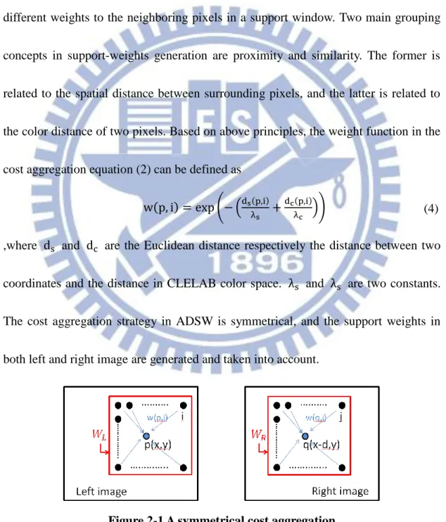
different weights to the neighboring pixels in a support window. Two main grouping

concepts in support-weights generation are proximity and similarity. The former is

related to the spatial distance between surrounding pixels, and the latter is related to

the color distance of two pixels. Based on above principles, the weight function in the

cost aggregation equation (2) can be defined as

w(p, i) = exp (− (ds(p,i)

λs +

dc(p,i)

λc ))

,where ds and dc are the Euclidean distance respectively the distance between two

coordinates and the distance in CLELAB color space. λs and λs are two constants.

The cost aggregation strategy in ADSW is symmetrical, and the support weights in

both left and right image are generated and taken into account.

Figure 2-1 A symmetrical cost aggregation

(18)

8

Figure 2-1 describes the symmetrical cost aggregation diagram. Let p and q be

respectively the center pixels in the current support window W_L in the left image and

the support window W_R in the right image. Then, the cost aggregation is rewritten as

following

𝐶

_𝑎𝑔𝑔

(𝑝, 𝑑) =

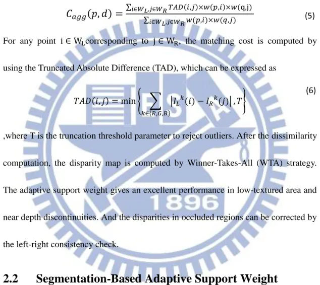
∑𝑖 𝑊𝐿,𝑗 𝑊𝑅𝑇 ( ,𝑗)×𝑤(𝑝, )×𝑤(q,j)

∑_{𝑖 𝑊𝐿,𝑗 𝑊𝑅}𝑤(𝑝, )×𝑤(𝑞,𝑗)

For any point i WLcorresponding to j WR, the matching cost is computed by

using the Truncated Absolute Difference (TAD), which can be expressed as

𝑇𝐴𝐷(𝑖, 𝑗) = min { ∑ |𝐼 (𝑖) − 𝐼 (𝑗)|

{ , , }

, 𝑇}

,where T is the truncation threshold parameter to reject outliers. After the dissimilarity

computation, the disparity map is computed by Winner-Takes-All (WTA) strategy.

The adaptive support weight gives an excellent performance in low-textured area and

near depth discontinuities. And the disparities in occluded regions can be corrected by

the left-right consistency check.

2.2 Segmentation-Based Adaptive Support Weight

In [8], Tombari et al. analysis the result obtained by the ADSW method. There

are some drawbacks in high-textured surfaces and repetitive patterns, since the

amount of aggregated support in ADSW may be insufficient in these regions. This is

because the use of spatial distance would determine the wrong support.

(5)

(19)

9

The basic idea of segmentation-based adaptive support is to embody the concept

of color similarity as well as segmentation information to improve the capability of

the support window. The proximity term has been eliminated from the support weight

computation. Instead, it is assumed that the disparity of each pixel has a similar value

in the same segment which can be obtained from a segmentation process, such as

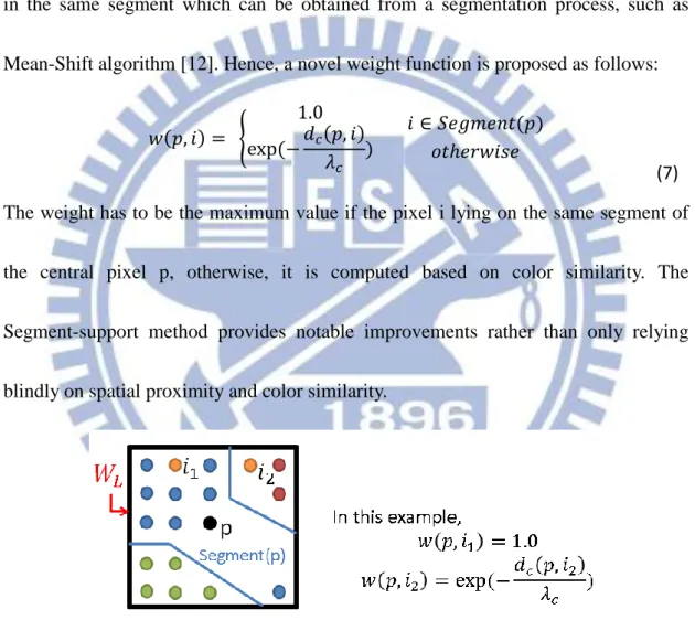
Mean-Shift algorithm [12]. Hence, a novel weight function is proposed as follows:

𝑤(𝑝, 𝑖) = { 1.0 exp (−𝑑𝑐(𝑝, 𝑖) 𝜆𝑐 ) 𝑖 𝑆𝑒𝑔𝑚𝑒𝑛𝑡(𝑝) 𝑜𝑡ℎ𝑒𝑟𝑤𝑖𝑠𝑒

The weight has to be the maximum value if the pixel i lying on the same segment of

the central pixel p, otherwise, it is computed based on color similarity. The

Segment-support method provides notable improvements rather than only relying

blindly on spatial proximity and color similarity.

Figure 2-2 A example for the segmentation-based adaptive weight generation

2.3 Mini-Census Adaptive Support Weight

The mini-census adaptive support weight method (MCADSW) [9] is an effective

algorithm modified from the ADSW method, and the former one has much lower (7)

(20)

10

complexity and more capability of dealing with brightness problem. The MCADSW

adopted the mini-census transform to improve the robustness to radiometric distortion.

Because mini-census cost measure has only relative information, a

scale-and-truncated approximation of the weight function is proposed. In addition, the

two-pass approach not only reduces computation complexity but also derives good

performance in low-texture areas.

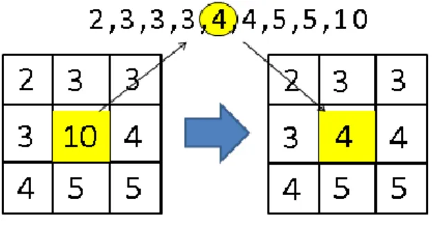
Figure 2-3 The mini-census transform and matching introduced in [9]

2.3.1 Mini-Census Transform and Matching

The concept of original census transform [3] is to obtain relative information instead of the intensity itself. The intensity used to compare is first transformed into Y color space. If a pixel’s intensity is larger than the center pixel’s intensity, it is

(21)

11

compares the intensity of the 6 significant pixels with the center pixel. After the

transformation, each pixel can be represented as a 6-bit binary bitstream. The

mini-census cost between the corresponding pixels is taken as the hamming distance

between two mini-census bitstreams, which is defines as 𝐶_𝑐(𝑝, 𝑑) = 𝑚( (𝑝), (𝑝 − 𝑑))

,where 𝐶 𝑐 represents the mini-census cost of pixel p with the disparity level d.

Ham() is the hamming distance function. (𝑝) and (𝑝 − 𝑑) are referred as the

bitstream of current pixel in the left image and the bistream of corresponding pixel in

the right image, respectively. An example of the mini-census transform and matching

introduced in [9] is shown in Figure 2-3. The mini-census cost performs better

disparity result in occluded area than the traditional SAD does.

2.3.2 Weight Generation

The weight function in the MCADSW method also eliminates the proximity

weight. Moreover, a scale-and-quantize weight function is defined as 𝑤(𝑝, 𝑖) = 𝑞 𝑛𝑡𝑖 𝑒 [𝑒 𝑝 (− (𝑝, )) × 𝑠𝑐 𝑖𝑛𝑔 𝑐𝑡𝑜𝑟]

The weight function is scaled up by 64 and quantized to leave only one nonzero most

significant bit. The purpose of scaling the function is to increase the influence of

neighbor pixel which has the small color distance.

(8)

(22)

12

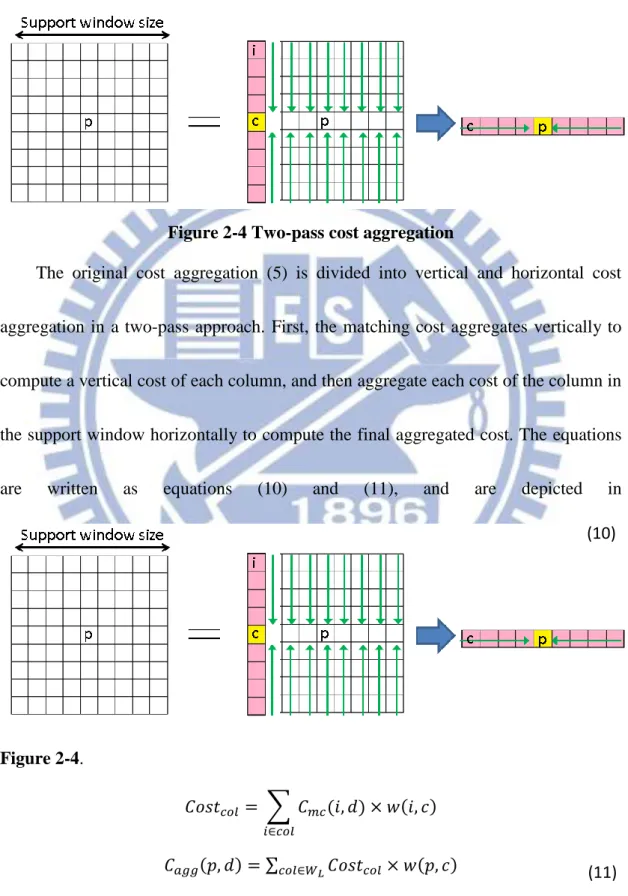
2.3.3 Two-pass Cost Aggregation

Figure 2-4 Two-pass cost aggregation

The original cost aggregation (5) is divided into vertical and horizontal cost

aggregation in a two-pass approach. First, the matching cost aggregates vertically to

compute a vertical cost of each column, and then aggregate each cost of the column in

the support window horizontally to compute the final aggregated cost. The equations

are written as equations (10) and (11), and are depicted in

Figure 2-4.

𝐶𝑜𝑠𝑡_𝑐= ∑ 𝐶_𝑐(𝑖, 𝑑) × 𝑤(𝑖, 𝑐)

𝑐

𝐶𝑎𝑔𝑔(𝑝, 𝑑) = ∑𝑐 𝑊𝐿𝐶𝑜𝑠𝑡𝑐 × 𝑤(𝑝, 𝑐)

where 𝐶 𝑐 is the mini-census cost defined in equation (8). Notice that c represents

(10)

(23)

13

the center pixel which changes column by column. Consequently, the MCADSW

method may improve the low-textured region with smoothing disparity, since the

correlated weight of the border or corner pixels could be increased with the help of

(24)

14

Chapter 3 Proposed Method

3.1 Motivation

In [7], the adaptive support weight can achieve the effect of using support

window with arbitrary sharp and give a quality depth result. Later, [2] proposed a

segment-based support weight to improve the performance. Mini-census transform in

[3] is employed to improve the capability of handling the lighting effect. However,

they all used a fixed support window size. According to our observation in Figure

3-1, , it shows that the performance will not always be better while the support

window size gets larger. This drawback is evident especially for Teddy and Cones

sequences. The issue of support window size still remains. Moreover, the mini-census

matching cost in [3] is much less sensitive to brightness bias, but it might cause errors

in low textured region since it lacks of color information.

According to the problems mentioned above, we proposed an algorithm which is

modified from the Mini-Census Support Weight (MCADSW) [3]. In the proposed

method, we combine the mini-census transform with the robust absolute differences

(RAD) measure to increase the robustness of the matching process. In addition, the

segment-based idea is inspired from [2] which apply the information obtained from

(25)

15

could determine the variable support window size instead of a fixed one. Besides, the

segment information can also be used for disparity refinement to improve the

performance of the final disparity result.

Figure 3-1 The performance comparison with different window size

0 5 10 15 20 25

nonocc all disc Average

Er ro r ra te(%)

Teddy

w=15 w=31 w=51 0 2 4 6 8 10 12

Venus

w=15 w=31 w=51 0 2 4 6 8 10 12 14

Tsukuba

w=15 w=31 w=51 0 2 4 6 8 10 12 14

Cones

w=15 w=31 w=51

(26)

16

3.2 The flow of the proposed method

Figure 3-2 The flow of the proposed algorithm

Figure 3-2 shows the flow of the proposed algorithm. First, we employ the

Mean-Shift algorithm to segment the inputted stereo images into regions according to

similar color. Second, the initial matching cost is computed by the combined matching

cost measure. After that, the weight generation and truncation step generates the

weight coefficients needed in the cost aggregation. Before the cost aggregation, we

employ the segment information to determine the support window size. And then, the

matching cost will be aggregated by a two-pass cost aggregation. Once the aggregated

(27)

17

(WTA) strategy. Finally, the result can be refined by left-right check and region-based

cross voting.

3.3 Robust matching cost computation

Mini-census cost transforms the intensity of the data term into relative bitstreams.

Hence it can tolerate outliers caused by radiometric noise. Nevertheless, it could also

lead to matching ambiguities in the regions with repetitive pattern, while the color

information can deal with these matching ambiguities. The idea of combining cost

measures for improved performance of matching process is inspired from the works

accomplished by Mei et al [13]. . They propose a combined cost measure with the AD

and census for matching cost initialization. The benefit of the combination is

impressive with a few additional computation time.

Based on MCADSW [9], we tend to preserve the mini-census cost measure Cmc

and combine with the color constraint. However, the origin AD cost range [0,255] is

much bigger than the mini-census cost range [0,6], so the combination cost might be

biased to the AD cost. Therefore, a robust function R is adopted for the AD measure

which maps the cost value range from [0,255] to [0,1]. It is defined as R(C_AD, λ_AD) = 1 − exp (−CAD

λ_AD)

,where CAD is the traditional AD cost described as equation (1), and 𝜆 is allowed

to control the influence of outliers. Given a pixel p with respect to a disparity level d, (12)

(28)

18

the proposed robust matching cost can be calculated as follows: 𝐶_{𝑏𝑢𝑠𝑡}(𝑝, 𝑑) = 𝐶 𝑐+ 𝜆 × 𝑅(𝐶 , 𝜆 )

,where 𝜆 is a tuning constant to control the influence between color similarity and

the relative information.

3.4 Weight generation and truncation

We exploit the weight function of the MCADSW described in equation (9), In

addition, a simple truncation is implemented to alleviate the matching error due to

outlier pixels. We give a minimum value zero to these outliers. Hence, a modified

weight function is proposed:

𝑤(𝑝, 𝑖 ) = {0 , 𝑖 𝑑𝑐(𝑝, 𝑖) > 𝑇𝑤 𝑞 𝑛𝑡𝑖 𝑒 [𝑒 𝑝 (− (𝑝, )) × 𝑠𝑐 𝑖𝑛𝑔 𝑐𝑡𝑜𝑟] , 𝑜𝑡ℎ𝑒𝑟𝑤𝑖𝑠𝑒

,where 𝑇𝑤 represents the threshold to separate the outliers; the cost 𝑑𝑐(𝑝, 𝑖) is sum

of color difference in YUV color space which is defined as

𝑑

_𝑐

(𝑝, 𝑖) = ∑

_{{𝑌,𝑈,𝑉}}

|𝐼

(𝑝) − 𝐼

(𝑖)|

The curve of our weight function is shown in Figure 3-3.

(13)

(14)

(29)

19

Figure 3-3 The curve of our proposed weight function

3.5 Support window size selection

The basic concept of the proposed method is to employ the segment information

to change the correlation window size. From our analysis, the MCADSW method still

suffers from some incorrect disparity estimation at occlusion, low textured, and

repeating pattern areas. Although we can improve the matching quality by applying a

larger supporting window, the disparity map might be blurred near the discontinuous

area.

3.5.1 Image segmentaion

The concept of the segmentation process is to cut the image into several regions

which can enlarge the region size as big as the spatial and color is assessed. In our YUV color difference

(30)

20

approach, we adopt the Mean-Shift algorithm to process the segmentation. Two

constant parameters σ_S and σ_R are referred as spatial radius and range radius

which construct the restraint of growing the segment. And the parameter 𝐹 𝑠𝑒

promises the minimum size of each region. Figure 3-4 shows the left image and its

segmentation result of each of four testing stereo images available on Middlebury

website [11], with the same parameter set: 𝜎𝑆 = 3, 𝜎 = 3, 𝐹 𝑠𝑒 = 35.

After the image segmentation step, the addition information of segment

represents an intelligent proximity rather than the spatial distance, and it can be

employed later in the support window size selection and the refinement step.

3.5.2 Variable window size selection

Instead of adopting a fixed support window size, the proposed method makes use

of information obtained from the Mean-shift algorithm to determine the support

window size. By observing the segment result shown in Figure 3-4, a large segment

is often related to a low textured or repeating area, where the support window should

be enlarged to obtain more support information. On the other hand, a small segment is

usually related to a border or occluded area. The MCADSW method can achieve the

window with arbitrary shape to deal with border area, and the occluded area can be

(31)

21

Hence, the window size selection can be expressed as:

𝑊 = {𝑊𝑠 𝑎 , 𝑖 𝑁 𝑚(𝑆𝑒𝑔(𝑝)) < 𝑇𝑐 𝑢𝑛𝑡 𝑊_{𝑏 𝑔} , 𝑜𝑡ℎ𝑒𝑟𝑤𝑖𝑠𝑒

Figure 3-4 The left image and the segmentation result of 4 stereo images

(32)

22

3.6 Two-pass cost aggregation

Once the window size is selected, the two-pass cost aggregation can be

processed. We adopt the same aggregation direction in [9] but simply modify the

original aggregation function (10)(11) with normalization after the cost aggregates.

The modified functions are described as equations (17) and (18):

𝐶𝑜𝑠𝑡

_𝑐

=

∑𝑖 𝑜𝑙𝐶_∑𝑅𝑜𝑏𝑢𝑠𝑡( , )×𝑤( ,𝑐) 𝑤( ,𝑐) 𝑖 𝑜𝑙

𝐶

_𝑎𝑔𝑔

(𝑝, 𝑑) =

∑ 𝑜𝑙 𝑊𝐶 𝑠𝑡 𝑜𝑙×𝑤(𝑝,𝑐) ∑ 𝑜𝑙 𝑊𝑤(𝑝,𝑐)

3.7 Disparity refinement

The disparity maps computed by the above steps contain errors in the occluded

and discontinuous regions. The results of left and right images are denoted as 𝐷 and

𝐷 , respectively. We refine the disparity errors by several steps. First, we smoothen the disparity map by a 3x3 median filter to alleviate the noise. Second, we detect the

outliers by the left-right check and then classify them into two categories. After that,

we treat the two kinds of outliers with different refinement rules. Finally, a

region-based cross voting refinement is performed. The first step has been introduced

in Figure 1-3, and the other steps are introduced as following.

(17) (18)

(33)

23

3.7.1 Left-right check and Outliers classification

Left-right consistency check [6] is a widely used technique to detect the outliers.

For each pixel, a following check is performed:

𝐷 (𝑝) = 𝐷 (𝑝 − (𝐷 (𝑝), 0))

If a pixel can’t satisfy the check, it is considered as an outlier. And then, based on the

method proposed by Hirschmϋller [14], we classify the outliers into “occlusion” and “mismatch” points. For each outlier pixel p, we perform the left-right check with all disparity candidates, and if no candidate could hold the check, p is an “occlusion”

pixel, otherwise a “mismatch” pixel.

Figure 3-5 demonstrates the classification results of four sequence on

Middlebury data sets compared with the occluded-region in the ground truth. If a

pixel is labeled as “occlusion”, we depict it with black color, and a “mismatch” pixel

is depicted with gray. The classification can effectively separate the occluded-region

which is similar to the ground truth.

(34)

24

Figure 3-5 The classification results(left) and the occluded-region in the ground truth(right)

3.7.2 Outlier refinement

The different kinds of outlier pixels require different refinement strategies.

(35)

25

horizontal scanline w that starts from the pixel p - (N,0) to the pixel p+(N,0).

And then we accept the disparity of q to p, which can be expressed as

𝐷

(𝑝) = {𝐷

(𝑞)|

min

𝑞 𝑝±(𝑁,0),𝑞≠𝑝

𝐶

(𝑝, 𝑞)}

2) If p is an occluded pixel, we first search the left and right nearest reliable

disparity, respectively denoted as 𝑆 and 𝑆₂. If only one reliable pixel is

found, 𝐷 (𝑝) is simply replaced by 𝐷 (𝑆 ) or 𝐷 (𝑆2). Otherwise,

𝐷 (𝑝) = min (𝐷 (𝑠 ), 𝐷 (𝑠2)) .

3.7.3 Region-based cross voting

Figure 3-6 Region-based cross voting

In this step, we reuse the segment information to further refine the disparity map.

For each pixel p, we build a histogram _𝑝 with DSR+1 bins for a cross voting

scheme, where DSR represents the disparity search range. The cross voting scheme is

depicted in Figure 3-6. We survey the neighbors both from the vertical and horizontal

directions, and collect the disparity votes if the neighbor q is located on the same

segment of p. After votes collection, the disparity candidate with the most votes is

(36)

26

Chapter 4 Experimental Results

To evaluate a stereo algorithm, a benchmark is provided on Middlebury Website

[11]. The four sequences, Tsukuba, Venus, Teddy, and Cones, are the most commonly

used for testing performance. For each image pair three error measures are proposed:

all image regions except for occlusions (nonocc), all regions (all), and near depth

discontinuities (disc). The default error threshold is set to 1.0.

In this section we present some experimental results of the proposed method.

The parameters are kept constant for all the data sets, which are presented in Table I.

𝜎_𝑆 𝜎 𝐹 𝑠𝑒 𝜆 𝜆 𝜆_𝑐

3 3 35 2 10 15

𝑇_𝑤 𝑊_{𝑠 𝑎} 𝑊𝑏 𝑔 𝑇𝑐 𝑢𝑛𝑡 N

100 31x31 51x51 300 15

Table I Parameter settings for the Middlebury evaluation

4.1 Evaluation of the robust matching cost measure

First we compare the MCADSW [9] result obtained from our implement and the

result after adopted the robust matching cost, which is referred as RCADSW. Both by

using the winner-take-all (WTA) strategy, Figure 4-1 shows the gain which comes

from the combined matching cost measure, and the gain is independent of the

(37)

27

Figure 4-1 The averaged error rate in different cost measure (w means the support window size)

0 2 4 6 8 10 12 14

A ve rag e E rr o r rate (% )

w = 15

RCADSW MCADSW 0 2 4 6 8 10 12

w = 31

RCADSW MCADSW 0 2 4 6 8 10 12 14

w = 51

RCADSW MCADSW

(38)

28

4.2 Compare the intermediate results of proposed method

In addition, we compared the intermediate and final disparity result of our

proposed method. The support window size is fixed as 31x31 both to MCADSW and

RCADSW. The results using variable window size method with and without the final

refinement are respectively denoted as “Proposed” and “Pro+refine”. The quantitative

evaluation of the intermediate and final disparity result is shown in Figure 4-2:

4 6 8 10 12 14 16 18 20

MCADSW RCADSW Proposed Pro+refine

e rr o r p e rc e n tage(% )

diparity estimation step

Teddy nonocc all disc Average 0 1 2 3 4 5 6 7 8

Venus

nonocc all disc

(39)

29

Figure 4-2 The error percentages of different error measures for 4 methods by our implementation

Table II lists the average bad pixels with average ranking of 4 methods are

respectively: Our MCADSW 7.57% (82.3), RCADSW 7.10% (74.7), proposed 6.8%

(67.3), pro+refine 5.63% (39.1). These experimental results show that the

performance can be improved by each step in the proposed algorithm.

0 2 4 6 8 10 12

Tsukuba

nonocc all disc 0 2 4 6 8 10 12 14

Cones

nonocc all disc

(40)

30

Table II Compared the results obtained from different step in the proposed algorithm

Algorithm

Tsukuba Venus Teddy Cones

non occ

all disc non occ

all disc Proposed 1.74 2.36 8.11 0.69 1.63 5.60 6.42 13.5 16.9 3.70 11.8 9.13

MCADSW [9] 2.80 0.64 13.7 10.1

SegmentSupport [8] 2.05 7.14 1.47 10.5 10.8 21.7 5.08 12.5 Table III Comparison between proposed method and the related works using winner-take-all before refinement step

Algorithm

Tsukuba Venus Teddy Cones Avg.

Bad Pixels Avg. Rank non occ

all disc non occ

all disc non occ all disc AdaptWeight [7] 1.38 1.85 6.90 0.71 1.19 6.13 7.88 13.3 18.6 3.97 9.79 8.26 6.67 64.6 SegmentSupport [8] 1.25 1.62 6.68 0.25 0.64 2.59 8.43 14.2 18.2 3.77 9.87 9.77 6.44 53.7 AdaptLocalSeq [15] 1.33 1.82 7.19 0.32 0.79 4.50 5.32 11.9 14.5 2.73 9.69 7.91 5.67 44.9 Proposed 1.74 2.36 8.11 0.69 1.63 5.60 6.42 13.5 16.9 3.70 11.8 9.13 6.80 67.3 Pro+refine 1.99 2.25 9.70 0.20 0.32 1.76 5.83 11.1 15.3 2.89 8.40 7.71 5.63 39.1

Table IV Quantitative Middlebury evaluation of the propose method and the state-of-the-art local method

Algorithm Tsukuba Venus Teddy Cones Avg.Bad

Pixels nonocc all disc nonocc all disc nonocc all disc nonocc all disc

Our MCADSW 2.71 3.33 11.1 0.62 1.50 5.16 6.75 14.5 18.4 3.91 12.4 10.4 7.57 RCADSW 2.37 2.93 10.3 0.84 1.86 7.26 6.35 14.3 17.1 3.23 11.6 8.76 7.10 Proposed 1.74 2.36 8.11 0.69 1.63 5.60 6.42 13.5 16.9 3.70 11.8 9.13 6.80 Proposed+refine 1.99 2.25 9.70 0.20 0.32 1.76 5.83 11.1 15.3 2.89 8.40 7.71 5.63

(41)

31

4.3 Compare with the reference works

Table III demonstrates the comparison between proposed method and the two

related work on the Middlebury stereo benchmark using a winner-take-all (WTA) rule.

The table also reports the results published in [8] and [9] without the refinement

process which consist only part of the error measures. As it can be seen from the table,

the proposed method produces a notable improvement on non-occluded and

discontinuous area compared to segment support method.

4.4 Compare with state-of-the-art methods

In the disparity refinement step, we fill the detected outliers with the reliable

neighbor pixels and introduce a histogram for cross voting procedure. Then, we

submit the obtained disparity maps to the Middlebury website and are compared to

the current state-of-the-art local methods. The quantitative Middlebury evaluation is

shown in Table IV. And the error percentages of different error measures for 4 test

stereo pairs in shown in Figure 4-3.

Finally, we show the disparity result obtained by the proposed method. From

Figure 4-4 to Figure 4-7 show the disparity maps and the corresponding error maps

(42)

32

error maps is evaluated by the default error threshold 1.0. The bad pixels are depicted

with gray color in occluded area, otherwise the black.

(a) Error rate of Teddy sequence

(b) Error rate of Teddy sequence 0 2 4 6 8 10 12 14 16 18 20

e rr or p e rcen ta ge (%)

Teddy

ADSW SegmentSupport AdaptLocalSeq Pro+refine 0 1 2 3 4 5 6 7

Venus

ADSW SegmentSupport AdaptLocalSeq Pro+refine

(43)

33

(c) Error rate of Teddy sequence

(d) Error rate of Teddy sequence

Figure 4-3 The error percentages of different error measures for 4 test stereo pairs obtained from different methods

0 2 4 6 8 10 12

Tsukuba

ADSW SegmentSupport AdaptLocalSeq Pro+refine 0 2 4 6 8 10 12

Cones

ADSW SegmentSupport AdaptLocalSeq Pro+refine

(44)

34

(a)Left image of Teddy (b) Ground truth

(c) result of ADSW [7] (d) Error map in [7]

(e) result of SementSupport [8] (f) Error map in [8]

(g) result of proposed method (h) Error map in proposed method

Figure 4-4 The disparity maps and the corresponding error map of our proposed method and related methods on Teddy sequence

(45)

35

(a)Left image of Venus (b) Ground truth

Figure 4-5 The disparity maps and the corresponding error map of our proposed method and related methods on Venus sequence

(46)

36

(a)Left image of Tskuuba (b) Ground truth

Figure 4-6 The disparity maps and the corresponding error map of our proposed method and related methods on Tsukuba sequence

(47)

37

(a)Left image of Cones (b) Ground truth

Figure 4-7 The disparity maps and the corresponding error map of our proposed method and related methods on Cones sequence

(48)

38

Chapter 5 Conclusion

In this paper, a combined matching cost measure with mini-census and color

difference is proposed. Moreover, we propose a variable window size selection

strategy before cost aggregation step. The strategy determines the support window by

utilizing the segment information derived from a color based segmentation method.

This information is also used for region-based cross voting scheme in refinement step.

Experimental results show that the proposed method effectively improves the

performance of original method in low textured region and near depth discontinuities. According the performance evaluation at the Middlebury website, the proposed

(49)

39

Reference

[1] M. Tanimoto, “Free viewpoint television - FTV,” in Proceedings of Picture

Coding Symposium (PCS), 2004.

[2] D. Scharstein and R. Szeliski, “A Taxonomy and Evaluation of Dense

Two-Frame Steroe Correspondence Algorithms,” International Journal of

Computer Vision, vol. 47, no. 1-3, pp. 7-42, 2002.

[3] R. Zabih and J. Woodfill, “Non-parametric local transforms for computing

visual correspondence,” in Proceeings of third European Conference on

Computer Vision, vol. 2, pp. 151-158, 1994.

[4] H. Hirschmϋller and D. Scharstein, “Evaluation of Stereo Matching Costs on

Images with Radiometric Differences,” IEEE Transactions on Pattern Analysis

and Machine Intelligence, vol. 31, no.9, pp. 1582-1599, 2009.

[5] Y. Boykov, O. Veksler, and R. Zabih, “Fast Approximate Energy Minimization

via Graph Cuts,” IEEE Transctions on Pattern Analysis and Machine

Intellgence, vol. 23, no. 11, November 2001.

[6] P. fua, “Combining Stereo and Monocular Information to Compute Dense

Depth Maps that Preserve Depth Discontinuities,” 12th International Joint

(50)

40

[7] K.-J. Yoon and I.-S. Kweon, “Adaptive Support-weight Approach for

Correspondence search,” IEEE Transactions on Pattern Analysis and Machine

Intelligence, vol.28, No.4, pp. 650-656, April 2006.

[8] F. Tombari, S. Mattoccia, and L. Di Stefano, “Segmentation-Based Adaptive

Support for Accurate Stereo Correspondence,” Lecture Notes in Computer

Science, vol. 4872, pp. 427-438, 2007.

[9] N. Y.-C. Chang, T.-H. Tsai, B.-H. Hsu, Y.-C. Chen, and T.-S. Chang, “Algorithm and Architecture of Disparity Estimation With Mini-Census Support Weight,” IEEE Transactions on Circuit and System for Video

Technology, vol. 20, no. 6, June 2010.

[10] Z.-F. Wang and Z.-G. Zheng, “A Region Based Stereo Matching Algorithm

Using Cooperative Optimization,” IEEE International Conference on Computer

Vision and Pattern Recognition, pp. 1-8, June 2008.

[11] D. Scharstein and R. Szeliski, “Middlebury stereo evaluation - version 2,”

http://vision.middlebury.edu/stereo/eval/, 2010.

[12] D. Comanicu, P. Meer, “Mean Shift: A Robust Approch Toward Feature Space

Analysis,” IEEE Transactions on Pattern Analysis and Machine Intelligence,

(51)

41

[13] X. Mei, X. Sun, M. Zhou, S. Jiao, H. Wang, and X. Zhang, “On building an

Accurate Stereo Matching System on Graphics Hardware,” Computer Vision

Workshops, pp. 467-474, 2011.

[14] H. Hirschmϋller, “Stereo Processing by Semiglobal Matching and Mutual

Information,” IEEE Transactions on Pattern Analysis and Machine Intelligence,

pp. 328-341, Feb. 2008.

[15] E.T. Psota, J. Kowalczuk, J. Carlson, and L. C. Perez, “A Local Iterative

Refinement Method for Adaptive Stereo Matching,” IPCV, 2011.

[16] F. Tombari, S. Mattoccia, L. Di Stefano, and E. Addimanda, “Classification and

Evaluation of Cost Aggregation Methods for Stereo Correspondence,” in

Proceedings of IEEE International Conference on Computer Vision and Pattern

基於區域可變式視窗大小和適應性權重的視差估計演算法

國立交通大學

資訊科學與工程研究所

碩 士 論 文

基於區域可變式視窗大小和

適應性權重的視差估計演算法

Region-Based Variable Window Size with Adaptive Support

Weight for Disparity Estimation Algorithm

研 究 生：黃致遠

指導教授：蔡文錦 教授

基於區域可變式視窗大小和適應性權重的視差估計演算法

Region-Based Variable Window Size with Adaptive Support Weight for

Disparity Estimation Algorithm

研 究 生：黃致遠 Student：Chih-Yuan Huang

指導教授：蔡文錦 Advisor：Wen-Jiin Tsai

國 立 交 通 大 學

資 訊 科 學 與 工 程 研 究 所

碩 士 論 文

中文摘要

ABSTRACT

誌謝

CONTENTS

LIST OF FIGURE

LIST OF TABLE

Chapter 1 Introduction

Chapter 2 Related Work

2.1 Adaptive Support Weight Approach

𝐶

(𝑝, 𝑑) =

2.2 Segmentation-Based Adaptive Support Weight

2.3 Mini-Census Adaptive Support Weight

2.3.1 Mini-Census Transform and Matching

2.3.2 Weight Generation

2.3.3 Two-pass Cost Aggregation

Chapter 3 Proposed Method

3.1 Motivation

Teddy

Venus

Tsukuba

Cones

3.2 The flow of the proposed method

3.3 Robust matching cost computation

3.4 Weight generation and truncation

𝑑

(𝑝, 𝑖) = ∑

|𝐼

(𝑝) − 𝐼

(𝑖)|

3.5 Support window size selection

3.5.1 Image segmentaion

3.5.2 Variable window size selection

3.6 Two-pass cost aggregation

𝐶𝑜𝑠𝑡

=

𝐶

(𝑝, 𝑑) =

3.7 Disparity refinement

3.7.1 Left-right check and Outliers classification

3.7.2 Outlier refinement

𝐷

(𝑝) = {𝐷

(𝑞)|

min

𝐶

(𝑝, 𝑞)}

3.7.3 Region-based cross voting

Chapter 4 Experimental Results

4.1 Evaluation of the robust matching cost measure

w = 15

w = 31

w = 51

4.2 Compare the intermediate results of proposed method

Venus

Tsukuba

Cones

4.3 Compare with the reference works

4.4 Compare with state-of-the-art methods

Teddy

Venus

Tsukuba

碩士論文

研究生：黃致遠

指導教授：蔡文錦教授

研究生：黃致遠 Student：Chih-Yuan Huang

國立交通大學

資訊科學與工程研究所

碩士論文