同心旋轉圓柱間調制Couette流及Taylor渦旋流之不穩定

國 立 交 通 大 學

機械工程學系

博士論文

同心旋轉圓柱間

調制Couette流及Taylor渦旋流之不穩定

Instabilities of Modulated Couette Flow and Taylor

Vortex Flow Between Concentric Rotating Cylinders

研 究 生:林豪傑

指導教授:楊文美 博士

同心旋轉圓柱間調制Couette流及Taylor渦旋流之不穩定

Instabilities of Modulated Couette Flow and Taylor Vortex

Flow Between Concentric Rotating Cylinders

研 究 生：林豪傑 Student：Hau-Chieh Lin

指導教授：楊文美 Advisor：Wen-Mei Yang

國 立 交 通 大 學

機 械 工 程 學 系

博 士 論 文

A Thesis

Submitted to Department of Mechanical Engineering College of Engineering

National Chiao Tung University In partial Fulfillment of the Requirements

for the Degree of Doctor of Philosophy

in

Mechanical Engineering

Nov. 2009

Hsinchu, Taiwan, Republic of China

同心旋轉圓柱間

調制Couette流及Taylor渦旋流之不穩定

學生:林豪傑

指導教授:楊文美 博士

國立交通大學機械工程學系博士班

摘要

同心圓柱間的旋轉流場在流體動力學之研究上處於極為重要之一

環，其有趣且複雜之現象，至今仍是眾多學者及研究人員相當關注的

研究課題。本論文主要目的為利用數值方法建構及分析不同半徑比之

同心圓柱間旋轉流場的型態，對於同心圓柱間多變之流況，以雷諾數

做為描繪流況之參數，探討此旋轉流場在調制與非調制轉速下之流動

特性。

本研究主題包括(1)不同調制效應的Couette流轉換為Taylor渦旋流

(2)調制與非調制Taylor渦旋流流場分析(3)非調制Taylor渦旋流轉換為

波動Taylor渦旋流。首先，針對在不同的調制振幅及頻率下的Couette

流進行穩定性分析研究，發生此不穩定將形成調制Taylor渦旋流。根據

Floquet理論可將擾動量分成時間與空間兩部份，其中時間函數與調制

具相同的頻率。數值方法採用Galerkin和Collocation法將擾動方程式轉

換為代數的特徵方程式，最後以QZ法求解特徵值，此複數型態特徵值

的實數部將為流場穩定與否的判斷指標。其次，探討調制與非調制

Taylor渦旋流場，在運算上直接求解二維、時變並以圓柱座標系統表示

的

Navier-Stokes 方 程 式 以 及 連 續 方 程 式 ， 其 中 數 值 方 法 是 以

Adam-Bashforth法和Crank-Nicolson法分別處理方程式中的非線性及線

性項，再將擾動方程式轉換為矩陣方程式並進行求解原始的壓力及速

度分量。最後，針對超臨界、軸對稱的非調制Taylor渦旋流進行穩定性

分析，求取在不同波數與半徑比下Taylor渦旋流轉換為波動渦旋流的最

低穩定曲線，在此階段主要以線性理論來簡化三維擾動的Navier-Stokes

方程式以及連續方程式，再利用Galerkin和Collocation等數值方法，將

擾動方程式轉換為代數的特徵方程式，如同第一階段Couette流場分析

準則，根據複數型態特徵值的實數部作為判斷Taylor渦旋流發生不穩定

之依據。

Instabilities of Modulated Couette Flow and Taylor Vortex

Flow Between Concentric Rotating Cylinders

Student：Hau-Chieh

Lin

Advisor：Dr. Wen-Mei Yang

Department of Mechanical Engineering National Chiao Tung University

ABSTRACT

Fluid flow between two concentric rotating cylinders has remained an important topic in fluid dynamics, attracting scholars and researchers to date. In this study, numerical methods are used to analyze and simulate flows and stabilities, which are characterized by a Reynolds number, under different radius ratios and modulated effects.

This study focuses on (1) the transition of Couette flow to Taylor vortex flow under different modulated amplitudes and frequencies, (2) the non-modulated and modulated Taylor vortex flows, and (3) the transition of the non-modulated Taylor vortex flow to wavy vortex flow.

First, the instability of modulated Couette flow before it transitions to modulated Taylor vortex flow, as well as the effects of modulated amplitude and frequency are studied. By using the Floquet theorem, perturbations are expanded into two series with time periodical coefficients which has the same period as that of the modulation. By following the work of Galerkin and using collocation methods, the equation is transformed into an algebraic eigenvalue problem. The QZ algorithm is employed to solve for the eigenvalues that determine the flow stability.

Second, the primitive variables of modulated and non-modulated Taylor vortex flows are solved numerically using the Crank-Nicolson and Adam-Bashforth methods to discretize the linear and nonlinear terms, respectively, of the Navier-Stokes equations.

Finally, the stabilities of supercritical Taylor vortex flows are studied by perturbing the nonlinear Taylor vortex flows. Using the same techniques as in part I, the marginal curves of transition to wavy vortex flows are obtained for different radius ratios and axial wave numbers. The resulting stability boundary curve for transition of supercritical Taylor vortex flow is different from that obtained in previous studies, in which the Reynolds number of the inner cylinder is assumed to increase quasi-statically.

致謝

取得學位的這條路這麼的漫長，無法置信的是我終於已經走到這個臨界點 了。內心有許多的感謝滿滿的一股腦想吶喊出來；謝謝文美老師您近幾年來的教 誨，在這領域的研究上之所以能夠紮穩根基，全然因為您的細心指導，雖然您平 日較不苟言笑，但我想這個表現還不算太差的學生畢業了，您應該可以放下心中 大石，微笑一下吧！我知道日後研究的路還很長，我不會令您失望的。 感謝武雄老師、雄略老師、慶耀老師及筱明老師蒞臨指導我的學位考試，經 由您的意見使我在這領域中更加豁然開朗，也學習到更多如何解決問題、表達結 果的技巧，謝謝各位老師的指導；也感謝曾經與我一同在實驗室共同打拼的學弟 們，讓我在實驗室中擁有溫暖的回憶。 當初斷然選擇退伍進而求取學位，主要為的就是想給家人一個不一樣的生 活，然而在這研修的道路上，並非全然平坦無阻，現實的生活曾給予我莫大的打 擊與壓力的負荷，然而一路走來，我的妻子-宜棻，始終如一的陪伴著我，她曾說 過他不是一個堅強的人，但我想對他說：若不堅強如妳，就不會有雙堅毅的推手 使我向前行，感謝妳的真心與無怨無悔的付出，今日與往後的所有榮耀完全歸功 於妳，謝謝妳！ 謹將本論文的研究成果獻給所有愛我及我所愛的父親、宜棻及最可愛的楚小 咪。

Table of Content

摘要

... i

 

ABSTRACT ... iii

 

致謝

...

v

 

Table of Content ... vi

 

List of Tables ... viii

 

List of Figures ... ix

 

Nomenclature ... xii

 

Chapter 1 Introduction ... 1

 

1.1 Motive of the Present Study ... 1 

1.2 Literatures Review ... 1 

1.3 Objective of This Study ... 6 

Chapter 2 Instability of Non-modulated and Modulated Circular

Couette Flow ... 7

 

2.1 General Features ... 7 

2.2 Numerical Procedures ... 7 

2.3 The Result of Non-modulated Effect on Couette Flow ... 13 

2.4 The Result of Modulated Effect on Couette Flow ... 14 

Chapter 3 Taylor Vortex Flow ... 36

 

3.1 General Description of the TVF ... 36 

3.2 Numerical Method ... 37 

3.2.1 Model description ... 37 

3.2.2 Governing Equations ... 37 

3.3 The Onset of Taylor Vortices under Modulated Effect ... 42 

3.4 Conclusion ... 44 

Chapter 4 Transition to Wavy Vortex Flow ... 57

 

4.1 The Second Transition of Taylor-Couette Flow ... 57 

4.2 Numerical Method ... 58 

4.2.1 Model Description ... 58 

4.2.2 Governing Equations ... 58 

4.2.3 Solution Method and Definition of Instability ... 63 

4.3 Lowest Instability of the Wavy Vortices under Inner Cylinder Rotation which is Re₁ ... 64 

4.4 The Lowest Instability Curve of the Transition from TVF to WVF under the Condition of Concerntric Rotating Cylinders ... 65 

4.4 Results Summary ... 66 

Chapter 5 Concluding Remarks ... 85

 

List of Tables

Table 1 Comparison list of results from this study and other scholars under the condition of a non-modulated Couette flow ... 18  Table 2 Radial velocity at the point of observation (ξ =0, z = 0) for η=0.5as

the outer cylinder is fixed and the inner cylinder rotates at a constant velocity. The definition of T_a is represented by

(

−η

)

(

+η

)

=21 Re2/1

a

T ... 45  Table 3 Comparison of experimental and theoretical data of Re values for

782 . 0 =

List of Figures

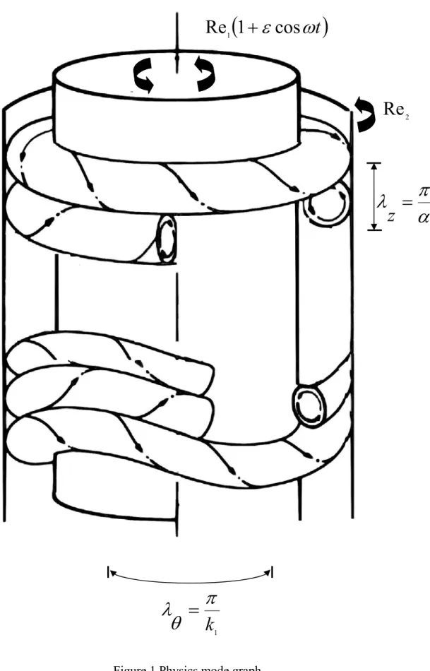
Figure 1 Physics mode graph ... 19  Figure 2 Coordinate graph ... 20 

Figure 3 (a) The relationship of relative variable  vs modulated frequency is showing under modulated effect  1 (b) A chart showing the variation of Re1 on different modulated amplitudes vs frequencies. (0.4833) ... 21 

Figure 4 Relationship between relative variable



of the Re1 and amplitude under different modulated effects. ... 23 

Figure 5 Different inner and outer radius ratios, and the relationship between critical Re and frequency. ... 27 

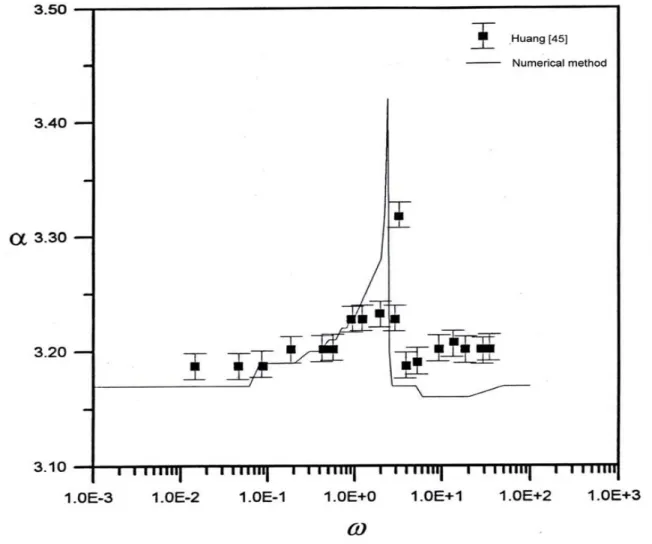
Figure 6 Influence of aspect ratio (h) on variable  of the critical Re (see Huang[45]). ... 28 

Figure 7 Influence of different upper and lower boundaries on variable  of the critical Re (see Huang[45]). ... 29 

Figure 8 Relationship between wave number of the modulated Couette flow under a stable critical number and modulated frequency; upper and lower fixed boundaries are  0.5and 48330. , respectively. ... 30 

Figure 9 Relationship between critical wave number and frequency at different modulated amplitudes. ... 31 

Figure 10 Relationship between the relative variable of the critical Re and frequency under different radius ratios. ... 34 

Figure 11 The relationship between offset of the critical Reynolds number  and modulated frequency when the outer cylinder is fixed and modulated amplitude of the inner cylinder is  1. ... 46 

Figure 12 The flow instability of the relationship between the rotating outer and inner cylinder. ( 0.937) ... 47 

Figure 13 The inner cylinder rotates with

  

_{1 1} , the outer cylinder

t ' 1 2  cos   

 rotates with a non-zero mean modulated rotation. The relationship between the Reynolds number of the inner cylinder and frequency. ( 0.937) ... 48 

Figure 14 The outer cylinder is fixed and the inner cylinder rotates at different modulated frequencies. The axial speed Vz



changes with time  at the point of observation ( 0.5, Z /4). (0.4833,  1) ... 49 

Figure 15 The outer cylinder is fixed and the inner cylinder rotates at different modulated frequencies. The axial speed Vz



changes with time  at the point of observation ( 0.5, Z /4). (0.4833,  2) ... 53 

Figure 16 Combines both numerical and experimental results for the onset of WVF for  0.893... 69 

Figure 17 Neutral stability curves of the transition of Taylor vortex flow to wavy vortex flow for various



. ... 70  Figure 18 The wave number of the lowest stability boundary for various. The

numbers denote k₁. ... 79 

Figure 19 The lowest stability boundary for the bifurcation from Taylor vortices. ... 80 

Figure 20 The lowest stability boundary for the bifurcation from Taylor vortices (with the simulated result obtained by Jones[34]). ... 81 

Figure 21 Different regimes in the flow between two rotating cylinders. 88

. 0 

 , 14.4. The fluid is silicone oil of 0.11 cm2/sec viscosity. Below the Taylor boundary there is circular Couette flow. Above the Taylor boundary there is axisymmetric Taylor vortex flow. Above the second boundary marked by the full circles there is

wavy (doubly periodic) Taylor vortex flow. After Coles [8] ... 82 

Figure 22 Lowest stability boundary for different azimuthal wavenumbers k ₁

corresponding to nonaxisymmetric TVF that is transformed to a WVF. ... 83 

Nomenclature

Alphabetic

d

gap of cylinders

h

aspect

ratio

1

k

azimuthal wave number (wavy mode)

2

k

axial wave number (wavy mode)

c

k

critical axial wave number ( for first transition)

p

pressure

P

pressure,

dimensionless

z

r ,,θ

cylindrical coordinates, dimensionless

R

radius of cylinder

Re

Reynolds

number

t

time

z r v v v , _θ,

velocity component

z r V V

V , _θ,

velocity component, dimensionless

Greek

α

wave

number

Δ

variation of critical Reynolds number

((Re_c−Re₀)/Re₀)

ε

modulated

amplitude

λ

wavelength

(

λ =2π/α

)

ν

dynamic

viscosity

coefficiency

ξ

collocation

coordinate

ρ

density

σ

growth rate of instability

τ

time,

dimensionless

ω

modulated frequency, dimensionless

'

ω

modulated

frequency

Ω

angular velocity of cylinder

Subscript

0

critical value, non-modulated

1 inner

cylinder

2 outer

cylinder

c

critical

value,

modulated

Superscript

Chapter 1 Introduction

1.1 Motive of the Present Study

Fluid flow between concentric rotating cylinders, generally known as circular Couette or Taylor-Couette flow (Couette[1]; Taylor[2]), is a classic problem in hydrodynamic stability and has provided an important paradigm for the dynamics of shear flows. This problem has been the focus of numerous theoretical and experimental studies.

Taylor[2] went one step further and studied the instability when both cylinders rotate. However, it is my opinion that the current problems concerning this instability (in particular the nonlinear problems) are outlined more clearly in the simpler case in which the outer cylinder is at rest. This strategy also is in line with the scientific paradigm of proceeding from the simple to the complex. Each additional variable makes the theoretical explanation of a nonlinear problem significantly more difficult.

The present study focuses on the centerpiece of the Taylor vortex problem, which is the instability of an infinitely long fluid column between concentric rotating cylinders. This instability is manifested in four ways: linear and nonlinear axisymmetric Taylor vortex flow (TVF), wavy vortex flow (WVF), irregular or chaotic Taylor vortex flow, and turbulent Taylor vortex flow. In this study, we only focus on the instability of the Couette flow, Taylor vortex flow, and wavy vortex flow and pursue the lowest instability boundary curves between these different types of flow.

1.2 Literatures Review

In this study, the behavior of flow motion for the following cases is investigated: (1) rotation of an inner cylinder, which remains static in an outer cylinder, (2) the inner and outer cylinders rotate at different speeds, and (3) the rotation of the inner cylinder is

periodic and modulated.

Donnelly[3] and Simon and Donnelly[4] utilized the torque produced in a cylinder during viscous flow motion to measure the circular Couette flow at the critical point between stable and unstable flow. As the rotational speed of the inner cylinder increases, the torque suddenly changes when the fluid status changes from stable to unstable. From this, the Reynolds number of the critical point can be acquired. The critical point marks the transition from one-dimensional stable Couette flow to two-dimensional Taylor vortex flow. Koschmieder[5], Burkhalter and Koschmieder[6], and Swinney and Gollub[7] obtained the same result by observing flows. For inner and outer cylinders with the same rotational speed and direction, Taylor[2] experimentally demonstrated that when the rotational speed increases gradually to a speed exceeding the critical speed, the flow still retains its one-dimensional flow status. In other words, the rotating outer cylinder has inhibition to stable status. Coles[8], Schwarz et al.[9], and Nissan et

al.[10] obtained the same experimental result as Taylor. Moreover, Walsh and

Donnelly[11] demonstrated that when the rotational speed of the inner cylinder is fixed and the outer cylinder undergoes periodic motion, the flow is stabilized. Gollub and Swinney[12] and Walden and Donnelly[13] used the Laser Doppler Anemometer (LDA) to investigate circular Taylor-Couette flow by measuring the radial temperature of flow measurement points.

Through power-spectrum analysis, the time domain is transformed into a frequency domain. The advantage of power spectrum analysis is that different characteristics of a spectrum represent different flow states. When flow is periodic, peaks of a certain size appear in the spectrum at relative and harmonic frequencies. When flow transitions into quasi-periodic flow, a new frequency appears that is not associated with the original frequency. The power spectrum analysis is an efficient approach for studying the

transformation between quasi-periodic and chaotic flows. Cole[14] experimentally investigated the effect of cylinder height on flow stability and demonstrated that cylinder height does not influence the critical point for transformation from a Couette flow to a Taylor vortex flow, unless the aspect ratio between cylinder height and interval is <8. Additionally, according to the study by Hall and Blennerhasset[15], when the aspect ratio L/d ≥12 12, the numerical and experimental results are not significantly different, indicating that the effect of cylinder height on flow stability is negligible. Barenghi and Jones[16] and Murray et al.[17] obtained the same result numerically. Walowit et al.[18] applied linear theory to derive the critical value for different radius ratios and the ratio between inner and outer rotational speeds. To examine the stability of a Couette flow between cylinders with different radial temperatures, Snyder and Karlsson[19] experimentally determined the critical Taylor

number ( 2

1 3 _{( / )}

2 Ω ν

= d R

Ta ) under different temperatures with η=0.958. They found that the result is stable over a small temperature range. Outside of this range, the positive and negative values of the critical Taylor number become unbalanced, and the flow typically becomes unstable.

The present study focuses primarily on the influence of modulated amplitude and frequency on flow stability between the cylinders. The rotational speed of the cylinder is

modulated by the factor _Ω−(1_+εcos_ω'_t) _{to investigate the effects of flow stabilization} and destabilization. Donnelly[20] experimentally analyzed modulated flow stability and found that when the outer cylinder remains static and the inner cylinder rotates periodically, parameters such as interval, rotational frequency, and modulation amplitude of the two cylinders can be modified to determine how the circular Couette flow is affected by modulated rotation. Hall[21] utilized linear theory to determine low and high frequencies and used non-linear theory to analyze the flow for high frequency

modulations. Hall demonstrated that flow is slightly destabilized regardless of amplitude for low frequency modulations. Within a certain frequency range, the flow becomes increasingly stable. When the rotation is modulated at high frequency, the stability approaches the critical value of the non-modulated situation. Riley and Laurence[22] utilized Galerkin expansion and Floquet theory for stability analysis and investigated flow stability under modulated conditions with a narrow inter-cylinder gap. The numerical result obtained by Riley and Laurence is the same as that acquired by Hall[21]. Davis[23] developed the notion of the quasi-steady limit by showing that a modulated inner cylinder destabilizes flow. Under extremely low frequency, the critical stability value of a flow declines to 1/(1+ε) of the non-modulated situation. Carmi and Tustaniwskyj[24] examined modulated flow stability under small-gap conditions and the influence of axis symmetry on modulated flow. In their study, the unstable offset of the critical Reynolds number increases at low frequencies. At medium-to-high frequencies, no stable critical value appears. Walsh and Donnelly[11] analyzed the flow between inner and outer cylinders with different radii using the photo voltage of observation particles. They determined that the critical Reynolds number has a relatively large offset at low frequency. In conclusion, a critical Reynolds number lower than the theoretical value indicates that the flow is temporarily unstable, but not permanently unstable. Therefore, the stable critical value is lower than the theoretical value at low frequency.

Walsh et al.[25] measured the critical Reynolds number for concentric cylinders with different radius ratios and, multiplying the result by a factor, obtained roughly the same value as that calculated by Carmi and Tustaniwskyj[24]. Kuhlmann et al.[26] utilized a low-dimensional model to examine the stability of circular Couette flow and Taylor vortex flow under instability. They found that a large modulated amplitude

causes subharmonic perturbation. Ganske et al.[27] used a static outer cylinder and a

modulated vortex flow in the inner cylinder to investigate the influence on stability of different amplitudes. They demonstrated that the modulated effect causes the flow to become increasingly unstable, and that the effect of amplitude on flow stability is significantly more important than the effect of frequency. When the amplitude is large, the unstable effect increases and the critical stability value declines further. Meksyn[28] used numerical methods to predict the occurrence of instability when the inner and outer cylinders rotated in either the same or opposite directions. Sparrow et al.[29] also applied numerical methods to investigate the same and opposite flows around inner and outer cylinders for a radius ratio of 0.95–0.1. Youd et al.[30], who analyzed zero-equivalent modulated flow around concentric cylinders with a radius ratio of

75 . 0 =

η , identified the axis symmetry of the Taylor vortex.

After the Taylor vortex problem had approached nonlinearity for many years, Coles[31] brought it decisively into nonlinearity in reporting the non-uniqueness of the wavy flow in the Taylor-Couette flow. The entire pattern of wavy vortices moves with uniform velocity in the azimuthal direction. Because the term “wavy” is typically associated with a motion that has periodic vertical oscillation, this study emphasizes that wavy Taylor vortices move in the azimuthal direction as rings that have an integer number k₁ of fixed sinusoidal upward and downward deformations (k₁ is the integer number of azimuthal waves). An example of a wavy Taylor vortex flow, as observed by Taylor[2], Lewis[32], Coles[31], and Schultz-Grunow and Hein[33], was not recognized as a characteristic new feature of the flow. After Coles’ preliminary results were published, wavy vortices were also observed by Nissan et al.[10]. Schwarz et al.[9] reported experiments in which they observed an asymmetrical mode with k₁ =1.

vortices with large radius ratios is independent of the Reynolds number in fluid columns of infinite length when the Reynolds number increases quasi-steadily. However, the wavelength of Taylor vortices is constant only as long as the flow is quasi-static. Jones[34] reported the stability boundary for wave number α =3.13, the critical value of a quasi-static transition, for a wide range of η.

Although Taylor analyzed the flow under supercritical conditions, Stuart[35] concluded that the vortex size remains unchanged above the critical Reynolds number. However, numerous studies (see Ahlers et al.[36], Andereck et al.[37], Park et al.[38], Burkhalter and Koschmieder [6, 39], and Antonijoan[40]) have demonstrated the importance of acceleration/deceleration in determining the final state of the flow. These vortices have axial wavelengths that are shorter or longer than those obtained after a quasi-static transition. This study demonstrates that the lowest stability boundary occurs at the critical wavelength of a quasi-static transition and also in another. These solutions are connected with standard Taylor vortices and can be obtained quasi-statically for certain radius ratios when using a mechanism to modify the axial wavelength (see Ref. [41]).

1.3 Objective of This Study

The literatures reviewed above describes the transition between Couette flow and supercritical Taylor vortex flow through experimental and theoretical work. However, the lowest-stability boundary between supercritical axisymmetric Taylor vortex flow to wavy vortex flow for different wave numbers and for various radius ratios is not clear. In this study, therefore, we will pursue the objective of the lowest stability curve for Taylor-Couette flow. This results will be compared with previous experimental and theoretical research.

Chapter 2 Instability of Non-modulated and Modulated

Circular Couette Flow

2.1 General Features

This study analyzes both fluid flow of rotating cylinders and the stability of modulated Couette flow by using numerical methods, under different modulated amplitudes and frequencies, the unstable behaviour caused by fluid flow and the influence to become a Taylor vortex flow is also studied. To investigate the change in stability of a modulated Couette flow, Floquet theorem is used with numerical methods. The amount of perturbation motion is divided into two progressions of time and space. Galerkin and Collocation techniques are then utilized to transform the perturbation motion formula into an algebraic Eigenvalue problem. Then QZ method is applied to solve the Eigenvalue problem. The factors of instability are determined by these Eigenvalues.

2.2 Numerical Procedures

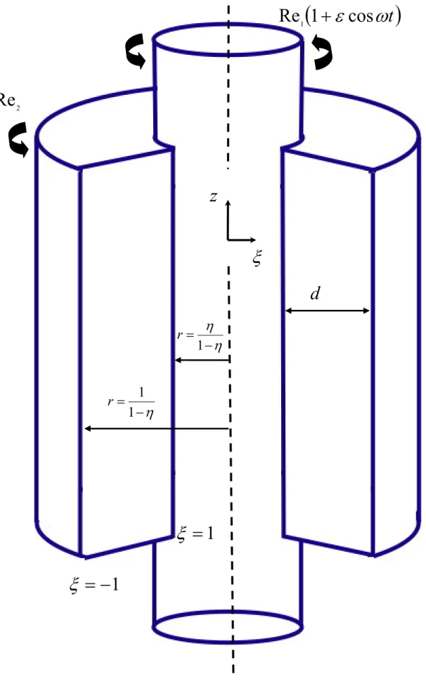
Figure 1 presents the physics model examined in this study. The two unlimited long vertical and concentric cylinders are full of viscid fluids. The outer cylinder remains static and the inner cylinder rotates at (1 cos ' )

1 +ε ωt

Ω . When the inner cylinder rotates at a fixed speed (ε =0) that is very low, the flow between cylinders is one-dimensional and stable. The fluid particles wind around the centre in a circular motion and is called a circular Couette flow. When rotational speed is increased to a critical value, the flow becomes unstable and forms a two-dimensional stable flow. At that time, the particles wind around the centre in toroidal motion; this is called a Taylor vortex flow (TVF). When the inner cylinder rotates in a modulated manner (ε ≠0) and average rotational

speed is very low, the flow remains one-dimensional; this is called a modulated circular Couette flow. When average rotational speed is increased to the critical value, the flow becomes unstable and is transformed into a two-dimensional flow. This critical rotational speed is affected by modulated amplitude ε and modulated frequency_ω'_.

For the convenience of problem analysis, we assume the working fluid is Newtonian fluid. Except for density, all other physical properties are fixed. The change in fluid density satisfies the Boussinesq approximation for gravity and centrifugal force; other items are ignored. The loss of fluid viscidly is also ignored. The governing equations are as follows: Continuity equation :

( )

1 0 1 ₌ ∂ ∂ + ∂ ∂ + ∂ ∂ z v v r rv r r z r _θθ (2.1) Momentum equations : = ∂ ∂ + ∂ ∂ + ∂ ∂ + ∂ ∂ z v v v r v r v v t v _r z r r r r θ θ ⎥ ⎦ ⎤ ⎢ ⎣ ⎡ ∂ ∂ − ⎟ ⎠ ⎞ ⎜ ⎝ ⎛ −∇ + ∂ ∂ − θ ν ρ r r v r v r r p 2 2 2 1 1 (2.2) = + ∂ ∂ + ∂ ∂ + ∂ ∂ + ∂ ∂ r v v z v v v r v r v v t v _r z r θ θ θ θ θ θ θ ⎥_⎦ ⎤ ⎢ ⎣ ⎡ ∂ ∂ − ⎟ ⎠ ⎞ ⎜ ⎝ ⎛ −∇ + ∂ ∂ ⋅ − θ ν θ ρ θ r v r v r p r 2 2 2 1 1 (2.3) = ∂ ∂ + ∂ ∂ + ∂ ∂ + ∂ ∂ z v v v r v r v v t v _z z z z r z θ θ z v z p_{+ ∇} ∂ ∂ − ν ρ 1 (2.4) Boundary condition : 1 R r = : v_r =v_z =0, v R

(

't

)

1 1 1 εcosω θ = Ω + (2.5) 2 R r = : v_r =v_θ =v_z =0 2 2 2 2 2 2 2 _{1 1} z r r r r ∂ ∂ + ∂ ∂ + ∂ ∂ + ∂ ∂ = ∇ θ (2.6)

the definitions of coordinates. the following parameters to make governing equation dimensionless: d R r= , d Z z= , ₂ d t ν τ = , ν ω ω=d2 ' , ν d R_{1 1} 1 Re = Ω (2.7) ν d v V r r = = , νθ θ v d V= = , ν d v V z z = = , ₂ 2 ρν pd P= = where d =R₂−R₁.

When inner cylinder rotates in fixed speed and the rotational speed is very low, the flow of cylinders is one-dimensional stable status and is called circular Couette flow. At that moment 0 = = r V , Vθ V_θ(r,τ) = = = , 0V=z = (2.8)

It is then substituted into dimensionless equation. After the simplification, the following is obtained: θ θ τ = = ⎟⎟ ⎠ ⎞ ⎜⎜ ⎝ ⎛ − + = V r dr d r dr d d V d 2 2 2 _{1 1} (2.9) Boundary condition: η η − = 1 r : V=r =V=z =0， θ =Re₁(1+εcosωτ) = V (2.10) η − = 1 1 r : V=r =V=θ =V=z =0

from the equation above, we can solve and get:

( )

(

)

₍

₎

₍

₎

1 2 2 _{1 1} 1 1 , − = − − + − − − = r r r V η η η η η η τ θ +

( ) ( )

( ) ( )

( ) ( )

( ) ( )

_⎭⎬⎫ ⎩ ⎨ ⎧ − − _ωτ ε _ei sr K sr I sr K sr I sr K sr I sr I sr K al 1 1 2 1 2 1 1 1 1 2 1 1 2 1 Re (2.11) where s= iω ， η η − = 1 1 r and η − = 1 1 2

cylinders respectively. I₁ and K₁ are respectively the first and second kind first order modulated Bessel functions.

According to the study by Carmi and Tustaniwskyj[24], axial symmetrical status is easily become unstable than axial asymmetrical status. Therefore, this study only considers disturbance as a symmetrical status. When the average rotational speed of a one-dimensional modulated circular Couette flow exceeds the critical value, the flow is transformed into a symmetrical two-dimensional flow. This flow can be considered a

one-dimensional flow ⎟ ⎠ ⎞ ⎜ ⎝ ⎛ = = P V ,0, ,

0 θ plus a disturbance

(

V_r',V_θ',V_z',P'

)

. At that moment, 0

= ∂

∂ θ . After substituting into the equation, simplification and ignoring the nonlinear items, the following disturbance equation is obtained:

Continuity equation:

( )

0 1 ' ₊ ' ₌ ∂ ∂ z r V rV r r (2.12) Momentum equations: ⎟⎟ ⎟ ⎠ ⎞ ⎜⎜ ⎜ ⎝ ⎛ − + ∂ ∂ + ∂ ∂ = = r V V z V V V _r z r ' ' 1 ' ₂ Re θ θ τ ⎥_⎦ ⎤ ⎢ ⎣ ⎡ ⎟ ⎠ ⎞ ⎜ ⎝ ⎛ −∇ + ∂ ∂ − = ' 2 ' ₁ r V r r P (2.13) ⎟⎟ ⎟ ⎠ ⎞ ⎜⎜ ⎜ ⎝ ⎛ ∂ ∂ + ⎟⎟ ⎟ ⎠ ⎞ ⎜⎜ ⎜ ⎝ ⎛ + ∂ ∂ + ∂ ∂ = = = z V V V r V r V V z r ' ' 1 ' Re θ θ θ θ τ ⎥_⎦ ⎤ ⎢ ⎣ ⎡ ⎟ ⎠ ⎞ ⎜ ⎝ ⎛ −∇ = ' 2 1 θ V r (2.14) ⎟⎟ ⎟ ⎠ ⎞ ⎜⎜ ⎜ ⎝ ⎛ ∂ ∂ + ∂ ∂ + ∂ ∂ = = z V V r V V V _z z z r z ' ' 1 ' Re τ ' ' z V z P _+∇ ∂ ∂ − = (2.15) Boundary condition: η η − = 1 r : ' ₌ ' ₌ ' ₌0 z r V V V _θ , η − = 1 1 r : ' ₌ ' ₌ ' ₌0 z r V V V _θ (2.16)

The variables _{P and} ' '

z

operation, and we can obtain ' 2 2 ₁ ) ( ) ( V_r r r r r z z _⎭⎬ ⎫ ⎩ ⎨ ⎧ ⎟ ⎠ ⎞ ⎜ ⎝ ⎛ ₊ ∂ ∂ ∇ ∂ ∂ − ∂ ⋅ ∂ ∂ + ∂ ⋅ ∂ ∂ ∂ ∂ τ τ z V r V z ∂ ∂ ⋅ ∂ ∂ − = ' 1 ) 2 (Re θ θ ₂ ' 2 2 1 z V r r ∂ ∂ ⎟ ⎠ ⎞ ⎜ ⎝ ⎛ −∇ = (2.17) ⎪⎭ ⎪ ⎬ ⎫ ⎪⎩ ⎪ ⎨ ⎧ ⎟⎟ ⎟ ⎠ ⎞ ⎜⎜ ⎜ ⎝ ⎛ + ∂ ∂ + ∂ ∂ = = ' 1 ' Re V_r r V r V V_θ θ θ τ ⎥_⎦ ⎤ ⎢ ⎣ ⎡ ⎟ ⎠ ⎞ ⎜ ⎝ ⎛ −∇ = ' 2 1 θ V r (2.18) ' r

V is the fourth order differential equation of r , and the boundary conditions are:

η η − = 1 r : ' ₌ ' ₌ ' ₌0 θ V dr dV V r r (2.19) η − = 1 1 r : ' ₌ ' ₌ ' ₌0 θ V dr dV V r r

The disturbance equation is the differential equation of time and space. Furthermore,

time and periodic coefficients are included in the equation. According to Floquet theory (Coddington and Levinson[42]]), the time item for disturbance can be divided into time and an index function, which increases over time. If the disturbance equation is described in normal mode, disturbance

(

'_, '

)

θ

V

V_r in the equation can be assumed in the axis direction and periodically distributed. Additionally, the index function increases over time, and the disturbance amplitude uses time and space as its function. The disturbance terms can be represented as

( )

( )

i z r _e r g r f V V _{στ α} θ τ τ ₊ ⎥ ⎦ ⎤ ⎢ ⎣ ⎡ = ⎥ ⎦ ⎤ ⎢ ⎣ ⎡ , , ' ' (2.20)

where α is the axial wave number, and σ is the growth rate of a complex disturbance. The stability of basic flow can be determined by the real number of the growth rate of a complex disturbance. When σ_r <0, the entire flow is stable. The disturbance declines as time increases. When σ_r >0, the disturbance increases over

time and the flow becomes unstable. When σ_r =0, the flow has neutral stability. The characteristic value of flow stability can be determined using the disturbance growth rate σ in the characteristic equation.

This study utilizes the spectral method (Canuto et al.[43]) to transform the

characteristic equation into an algebraic characteristic equation. The QZ numeric method is then applied to solve the characteristic value of this equation group. According to the Floquet theory,

[

f

( ) ( )

r,τ ,g r,τ

]

represents the disturbance value. The second orders of time and space are expanded. Time is expanded via a complex Fourier series of period 2π ω. Space is expanded by the first type n orders of Chebyshev polynomial (Fox and Parker[44]). The definition of Chebyshev polynomial is

( )

ξ _=cos

(

_n⋅cos−1ξ

)

T_n (2.21)

The defined domain of r in the original equation is transformed from

(

η

)

(

η

)

η/1− ≤r≤1/1− to −1≤ξ ≤1 through the relational equation

(

η

) (

η

)

ξ =2r− 1+ /1− . The amplitude in normal mode can be expressed as

( )

_{ξ τ}

( )

_ξ imωτ n m n mn e a f ∞ − −∞ = ∞ = Ψ =

∑ ∑

4 , (2.22)

( )

_{ξ τ φ}

( )

_ξ imωτ n m n mn e b g ∞ − −∞ = ∞ =

∑ ∑

= 2 , (2.23)

where a and _mn b are unknown coefficients, and _mn Ψ and _n φ_n are basis functions. The definition of the basis functions are as follows:

⎪ ⎪ ⎩ ⎪ ⎪ ⎨ ⎧ ⎟⎟ ⎠ ⎞ ⎜⎜ ⎝ ⎛ − − + − − ⎟⎟ ⎠ ⎞ ⎜⎜ ⎝ ⎛ − + − = Ψ 1 2 3 2 0 2 2 2 1 8 1 8 1 1 4 4 T n T n T T n T n T n n n n≥4 (2.24) ⎩ ⎨ ⎧ − − = 1 0 T T T T n n n φ n≥2 (2.25) for even n for odd n for even n for odd n

The Galerkin and collocation methods are applied to make the characteristic equation discrete, and can be represented by a matrix such as

~ ~ ~ ~ Y B Y A =σ (2.26)

where σ is the characteristic value used to determine flow stability in this study.

⎥ ⎦ ⎤ ⎢ ⎣ ⎡ = 11₂₁ 12₂₂ ~ A A A A A , _⎥ ⎦ ⎤ ⎢ ⎣ ⎡ = ₂₁11 ₂₂12 ~ B B B B B , ⎥ ⎥ ⎦ ⎤ ⎢ ⎢ ⎣ ⎡ = ~ ~ ~ b a Y (2.27)

2.3 The Result of Non-modulated Effect on Couette Flow

Table 1 shows experimental results. The flow generates an unstable critical value and average experimental value of Re₀ =68.75. Compared with experimental results obtained by other studies, the error rate is < 1.18%. If error deviation is added, then the critical value is Re₀ =68.75±1.1. The experimental results acquired by other studies are within the error range in this experiment. The experimental result is the experimental foundation of the modulated Couette flow. For measurement of wave number α , only the total length of 10 cells in the middle of the flow (equivalent to the total length of five wavelengths) were examined to avoid influence from upper and lower boundaries in the experiment. The vortex size is averaged and then its wavelengthλ is calculated. The precision of this measurement is within 0.1mm. Then, the wavelength is calculated by λ =2π/α.

Table 1 shows the average wave number, which is α =3.19. The theoretical value calculated for unlimited length is α =3.17. The error between the experimental result and theoretical value is < 0.6%. Additionally, this experiment also examined different aspect ratios, including h=24, 20 and 16. The experimental result does not change obviously and the critical Re is within 68.75±1.1. Therefore, the aspect ratio does not have a significant effect on the aspect ratio; this is the same experimental result obtained

by Cole[14].

2.4 The Result of Modulated Effect on Couette Flow

Under a modulated effect, the inner cylinder rotates with the (1 cos ' ) 1 +ε ωt Ω

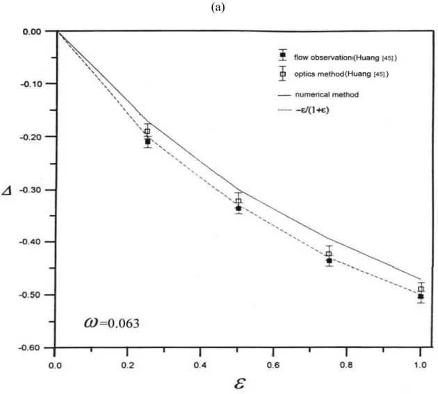
period. The stability of the modulated Couette flow is primarily affected by modulated amplitude and modulated frequency. This study analyzed different aspect ratios, upper and lower boundaries to determine how they affect the modulated Couette flow. To compare modulated effect with the non-modulated effect, the change rate of the critical Re1 is defined here; Δ =(Re_c−Re₀)/Re₀ , Δ>0 represents the modulation has stabilized.

The experimental value was obtained using the optical measurement method and flow observation method. The solid line on Fig. 3(a) is the theoretical result. At a low frequency, when Δ < 0, the critical Re is lower than that for a non-modulated effect. The result demonstrates that the modulated effect has an unstable effect on flow. Additionally, when the frequency continues to decrease, Δ approached the quasi-static limit )−ε/(1+ε . At a medium-to-high frequency, Δ increases as frequency increases. Generally, in this frequency range, the modulated effect destabilizes the flow. As frequency decreases, destabilization increases.

The error of result in this experiment and theoretical value are relatively large at a medium frequency (Fig. 3(a)). At a high frequency, Δ approaches but remains slightly lower than 0. At that moment, modulated frequency has slightly destabilized the flow. Figure 3(b) presents the curve of medium stable critical Re at different modulated amplitudes. When the flow is unstable, the disturbance has three statuses. For any amplitude, disturbance σ_i =0 at a low frequency is synchronous. After the flow becomes unstable, the frequency of the flow and base status are the same. As frequency

increases, disturbance changes to a quasi-periodic state. At that moment, σ_i ≠0 and the ratio of the flow frequency to base status frequency is not a rational number. When the frequency increases to an ultra-high frequency, σ_i is multiple times the base status frequency. At that moment, disturbance returns to synchronous.

Figure 4 shows the relationship between relative variable Δ of the Re and amplitude under different frequencies. The solid line in the graph is the experimental result derived using the numerical method. The dotted line in Fig. 4(a) is the quasi-steady limit −ε/(1+ε)when ω→0. At an extra low frequency, if the amplitude is high, destabilization is also high. If the critical Re approaches Re₀/(1+ when ε) frequency is ω=0.063, amplitude increases from 0 to 1.0, and the variable Δ of the Re1 gradually decreases to around −0.5. Additionally, based on the graph, the experimental result and quasi-static limit −ε/(1+ε) are extremely close. When the modulated frequency is ω =0.628 and ω=6.28(Figs. 4(b) and 4(c), respectively), the relative variable Δ of the Re1 will decrease as modulated amplitude increases. When the modulated amplitude is high, the relative variable Δ of the Re decreases and the flow becomes increasingly unstable. However, the degree of instability is lower than that at a low frequency.

At a high frequency (Fig. 4(d)), when modulated frequency is ω =62.8, the different modulated amplitude does not have a significant effect on relative variable Δ of the Re. The modulated amplitude does not significantly influence flow stability.

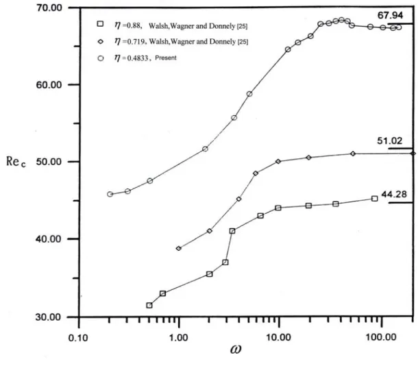
For different radius ratios η, Fig. 5 presents the experimental result obtained by this study and Walsh et al.[25]. The graph includes different radius ratios η, which include η = 0.4833, 0.719, 0.88, and a modulated amplitude of 0.5. Regardless of the radius ratio, the stable critical value increases as frequency increases, and approaches a

stable critical value Re under the non-modulated effect. At a low frequency, the ₀ stable critical value approaches Re₀/(1+ . ε)

This study investigated the influence of several aspect ratios h on the stable critical value. Figure 6 presents numerical results. When aspect ratio h decreases, Δ also decreases and flow destabilization increases. When frequency is high, the rate reduction is obvious.

This experiment chose three different cylinder boundary conditions: fixed on sides, top free bottom fix, and top rotate bottom fix. The aspect ratio is h=24. Figure 7 presents the numerical result. The measured results for the three conditions are similar. The flow is not affected by the upper and lower boundaries. The possible reasons are that measurement points for the optical measurement method are at the middle of the cylinder and the aspect ratio is sufficiently large. Therefore, the effect caused by boundaries near measurement points is extremely small.

For the non-modulated effect, the experimental result for wave number of the stable critical value is α =3.19. When the flow is modulated, the flow observation method is used to measure the wave number when flow exceeds a stable state, and determine whether the wave number changes under a modulated effect. Figure 8 shows numerical results. The wave number first decreases as the modulated frequency increases. The wave number is not a fixed value and changes for different modulated frequencies. The degree of change to experimental data is not as large as the theoretical value; however, the tendencies are the same.

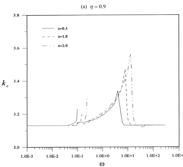
Figure 9 presents the relationship between critical wave number k and frequency _c

for different radius ratios and modulated amplitudes. When the flow transforms disturbance from synchronous to quasi-periodic, a discontinuous point exists at amplitude. The axial wave number increases as modulated frequency increases. When

the frequency exceeds the first discontinuous point, axial wave number suddenly decreases and then increases again. When the axial wave number reaches a maximum value, the critical Re also reaches a maximum value, the decrease as modulated frequency increases. Finally, the axial wave number approaches the value of non-modulated rotation at an extra high frequency.

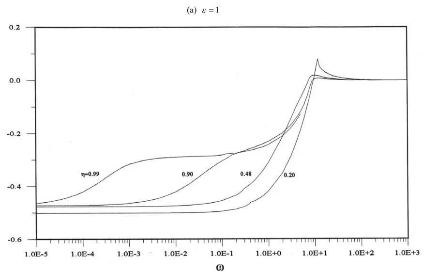
Figure 10 presents the relationship between the Re1 and frequency when amplitude is (a)ε =1 and (b)ε =2 under different radius ratios η. When radius ratio η is small, the change to the critical Re under medium-to-high frequency becomes steep; at a stable status, the offset is large.

Table 1 Comparison list of results from this study and other scholars under the condition of a non-modulated Couette flow

Study method Aspect ratio Radius ratio Critical value Wave number h η Re 0 α

Huang[45] Flow visualization and Optical method

24 0.4833 68.75 3.19

Donnelly[3] Torsion measurement

method 4 0.5 68.28

Donnelly[46] Flow visualization 5 0.5 68.57 3.10

Simon and Donnelly[4] Torsion measurement method 5 0.5 68.23 Sparrow et al.[29]

Numerical method Infinite 0.5 68.19 3.16

Present Numerical method Infinite 0.4833 67.94 3.17

Re

₂

Figure 1 Physics mode graph

(

1

ε

cos

ω

t

)

Re

₁

+

1

k

π

θ

λ

=

α

π

λ

=

z

Re

₁

(

1

+

ε

cos

ω

t

)

z

ξ

d

η

η

− = 1 r

η

−

=

1

1

r

ξ

=

1

ξ

=

−

1

Figure 2 Coordinate graph 2

(a)

Figure 3 (a) The relationship of relative variable Δ vs modulated frequency is showing under modulated effect ε =1 (b) A chart showing the variation of Re1 on different modulated amplitudes vs frequencies. (η=0.4833)

(b)

(a)

Figure 4 Relationship between relative variable

Δ

of the Re1 and amplitude under different modulated effects. (a) ω =0.063 (b) ω =0.628 (c) ω =6.28 (d) ω =62.8

(b)

(c)

(d)

Figure 8 Relationship between wave number of the modulated Couette flow under a stable critical number and modulated frequency; upper and lower fixed boundaries are ε =0.5and 4833η=0. , respectively.

(a) η =0.9

Figure 9 Relationship between critical wave number and frequency at different modulated amplitudes. (a) 9η =0. (b) η =0.4833 (c) η=0.2

(b) η =0.4833

(c) η =0.20

(a) ε =1

Figure 10 Relationship between the relative variable of the critical Re and frequency under different radius ratios. (a) ε =1 (b) ε =2

(b)

ε

=

2

Chapter 3 Taylor Vortex Flow

3.1 General Description of the TVF

Fluid motion between two concentric rotating cylinders is often investigated in the field of fluid dynamics. This section uses numerical methods to analyze and simulate flow patterns and relevant flow characteristics between two concentric rotating cylinders. Coles[8] was the first researcher to definitively consider Taylor vortex flow to be nonlinear, although several researchers had previously speculated that the Taylor vortex problem could be solved by considering nonlinear flow. Donnelly[47] and Hu[48] experimentally analyzed modulated flow stability. When the outer cylinder remains stationary and the inner cylinder rotates periodically, parameters such as interval, rotational frequency, and the modulated amplitude of the two cylinders can be varied to determine how the flow is affected by modulated rotation. Hall[21] utilized linear theory to determine low and high frequencies and used nonlinear theory to analyze the flow under a high frequency. Carmi and Tustaniwskyj[24] examined modulated stability under a limited gap and the influence of axial symmetry and asymmetry on modulated flow. In a former study, it was shown that the critical Reynolds number exhibits an increased unstable offset under low frequency. Marques and Lopez[49] and Lopez and Marques[50] introduced and studied more cases of time-modulated Taylor–Couette problems in which the inner cylinder moves periodically along the axial direction. Youd

et al.[30, 51], who analyzed zero-equivalent modulated flow around concentric

cylinders with a radius ratio of η=0.75, defined as η =R₁/ R₂ where R and ₁ R , ₂

are the inner and outer radii of cylinders, identified the formation of reversing and non-reversing modulated Taylor–Couette flow. The main objectives of the study investigate the instability of modulated Taylor vortices flow by utilizing a numerical

method. It is practical to focus attention on the transition based on varying modulated amplitudes and frequencies.

3.2 Numerical Method 3.2.1 Model description

The flow is described by the incompressible, three-dimensional Navier-Stokes equations with cylindrical coordinates ( R , θ , Z ) in an absolute frame of reference according to the velocity-pressure formulation. The dimensionless factors r , z are the radial and axial coordinates, τ is the time and ω is the modulated frequency with corresponding dimensional quantities are t and _ω'_{; Re is the Reynolds number of} the inner cylinder and α is the axial wave number; the velocity components and

pressure are Vr − , θ − V , Vz − , and P . − 3.2.2 Governing Equations

The basic flow type is the one-dimensional Couette flow with the modulated amplitude and frequency of azimuthal velocity between two concentric cylinders. Then the inner cylinder rotates with the increasing Reynolds number Re, and the outer cylinder is considered to be at rest under all conditions. The dimensionless Navier-Stokes and continuity equations are as follows:

→ − → → → Δ + −∇ = ⎟ ⎠ ⎞ ⎜ ⎝ ⎛ ∇⋅ + ∂ ∂ V P V V t V Re 1 , ∇⋅V→ =0 (3.1) where _⎟ ⎠ ⎞ ⎜ ⎝ ⎛ = − − − → z r V V V

V , θ, . The time scheme is semi-implicit and second-order accurate. It corresponds to a combination of the Crank-Nicolson scheme (for the linear term) and an explicit Adam-Bashforth scheme (for the nonlinear terms).

Cole [14] demonstrated that cylinder height does not influence the critical point for transformation from a Couette flow to a Taylor vortex flow unless the aspect ratio between cylinder height and interval is less than 8. We assume infinite cylinders and a periodic solution in the axial direction. The boundary conditions are

η η − = 1 r : V−r =V−z =0, θ =Re₁

(

1+εcosωτ

)

− V η − = 1 1 r : V→=0 (3.2)

where ε and ω are the modulated amplitude and frequency, respectively.

The flow velocity and pressure profile of the Taylor vortices can be regarded as a one-dimensional flow with a perturbation and can be expressed as:

(

, ,τ

)

0 _V' _{r z} Vr = + _r − (3.3)

( )

τ _θ

(

τ

)

θ θ V r, V' r,z, V− = = + (3.4)

(

, ,τ

)

0 _V' _{r z} Vz = + _z − (3.5)

(

, ,τ

)

0 _p' _{r z} P− = + (3.6)

The perturbations are determined using a pseudo-spectral Fourier-Chebyshev collocation method, taking advantage of the orthogonality properties of Chebyshev polynomials and assuming exponential convergence (see Daoyi and Gerhard H.[52], Speetjens and Clercx[53]).

( ) ( )

m z A V M m n N n mn r τ φ ξ cos α 1 0 1 2 '

∑∑

− = + = = (3.7)

( ) ( )

m z B V M m n N n mn τφ ξ α θ cos 1 0 1 2 '

∑∑

− = + = = (3.8)

( ) ( )

m z C V M m n N n mn z τ φ ξ sin α 1 1 2 '

∑∑

= + = = (3.9)

( ) ( )

T m z D p M m n N n mn α ξ τ cos 1 0 1 0 '

∑∑

− = − = = (3.10)

Here, M and N are the number of terms in the Fourier series expansion and Chebyshev polynomial expansion, respectively, and A , _mn B , _mn C , and _mn D are _mn

amplitude coefficients. The definitions of Tn and φn are listed in section 2. Vθ

( )

r,τ

=

is the velocity of one-dimensional Couette flow.

Substituting Eqs. (3.3)–(3.6) into the Eq. (3.1), the equations are transformed into an algebraic equation, which can be expressed as a matrix equation:

1 , 1 − + ₌ j j j _F AX , ⎥ ⎥ ⎥ ⎥ ⎦ ⎤ ⎢ ⎢ ⎢ ⎢ ⎣ ⎡ = 0 0 0 0 0 0 0 0 0 43 41 34 33 22 14 11 A A A A A A A A , ⎥ ⎥ ⎥ ⎥ ⎦ ⎤ ⎢ ⎢ ⎢ ⎢ ⎣ ⎡ = mn mn mn mn D C B A X , ⎥ ⎥ ⎥ ⎥ ⎦ ⎤ ⎢ ⎢ ⎢ ⎢ ⎣ ⎡ = 0 3 2 1 F F F F (3.11)

where A is a matrix of coefficients and vector X =

(

A_mn,B_mn,C_mn,D_mn

)

T . The unknown values of vector F , _F

(

_{F ,F ,F ,0}

)

T

3 2 1

= , are the summation of radial, azimuthal and axial velocity components for linear term at time t_j and nonlinear term at time t_j−1. n r m D r D d A τ α _⎥φ ⎦ ⎤ ⎢ ⎣ ⎡ ⎟ ⎠ ⎞ ⎜ ⎝ ⎛ _{+ − −} − = 2 2 2 ₂ 11 1 1 2 1

(

DTn

)

d A₁₄ = τ n r m D r D d A τ α _⎥φ ⎦ ⎤ ⎢ ⎣ ⎡ ⎟ ⎠ ⎞ ⎜ ⎝ ⎛ _{+ − −} − = 2 2 2 ₂ 22 1 1 2 1 n m D r D d A τ α _⎥φ ⎦ ⎤ ⎢ ⎣ ⎡ ⎟ ⎠ ⎞ ⎜ ⎝ ⎛ _{+ −} − = 2 2 2 33 1 2 1

(

m

)

Tn d A₃₄ = τ − α n D r A ⎟φ ⎠ ⎞ ⎜ ⎝ ⎛ + = 1 41

n m A₄₃ = αφ = 1 F j mn nA r m D r D dτ _{α φ} ⎥ ⎦ ⎤ ⎢ ⎣ ⎡ ⎟ ⎠ ⎞ ⎜ ⎝ ⎛ _{+ − −} − 2 1 2 2 1₂ 2 1 d

(

R V j Rj V_rj m z

)

r j _α τ cos , 3 2 1 ' 1 ' ₋ − − −

(

V V m z

)

r d j j α τ θ θ ,cos 3 2 1 2 ' 2 ' ₋ − − _⎟⎟ ⎠ ⎞ ⎜⎜ ⎝ ⎛ − − ₆ − ₂− −1 −1 2 j mn n j j mn n j B V B V r dτ _{φ φ} θ θ = 2 F j mn nB r m D r D dτ _{α φ} ⎥ ⎦ ⎤ ⎢ ⎣ ⎡ ⎟ ⎠ ⎞ ⎜ ⎝ ⎛ _{+ − −} − 2 1 2 2 1₂ 2 1 ⎟⎟ ⎠ ⎞ ⎜⎜ ⎝ ⎛ ⎟ ⎠ ⎞ ⎜ ⎝ ⎛ ₊ − ⎟ ⎠ ⎞ ⎜ ⎝ ⎛ ₊ − − _V − _V − _{m z} r R V V r R d j j r j j j r j _α τ θ θ 1 ,cos 1 3 2 1 ' 1 ' 2 1 ' ' 2 = 3 F j mn nC m D r D dτ _{α φ} ⎥ ⎦ ⎤ ⎢ ⎣ ⎡ ⎟ ⎠ ⎞ ⎜ ⎝ ⎛ _{+ −} − 2 1 2 2 2 1 d

(

R V j Rj V_zj m z

)

z j _α τ cos , 3 2 1 ' 1 ' ₋ − − − where n n n n n _d D d r = = ∂ ∂ ξ 2 , z V r V Rj _rj _zj ∂ ∂ + ∂ ∂ = ' ' _and

(

)

= =

_∫

₋α π ⋅ π α π α / / 2 ,g f g f gdz f _o

The coefficients A ,_mn B ,_mn C , and _mn D are determined iteratively until the _mn

convergence condition is satisfied. When the inner cylinder rotates with a fixed rotational speed, the convergence condition is

4 1 1 10− + + < − j j j X X X (3.12)

We adopt the tolerance (10-4) to avoid the computation process becomes time consuming and larger error ratio compared with those obtained by Jones [54]. When the pressure coefficient is converging to the tolerance (10-4_{), the other coefficients in} velocity components had been converging and lower to the tolerance (10-4). The coefficient that satisfies the convergence condition is substituted in the appropriate equation among Eqs. (3.3)–(3.6); the speed and pressure in each time interval can then be determined. If the cylinder rotates periodically, the largest value of axial speed

attained in a particular time interval at a selected observation point in the flow is compared with the axial speed in the preceding time interval, the convergence condition is 4 1 1 10− + − − + − < − i z i z i z V V V (3.13)

where i is the periodic counter. If the difference is less than ₁₀−4 _{, then the} convergence condition is considered to be satisfied.

3.2.3 Model Validation

Prior to the computation of the flow field, we analyze the degree of accuracy, which serves as the basis for the post computation. In theory, the greater the number of terms expanded, the higher is the accuracy; however, the limit to the increase of the number of terms will come from the round-off error and the computation process becomes time consuming. Therefore, the best option is to use the expansion with the least number of terms for which a certain degree of accuracy can be guaranteed. The results computed from the expanded number of terms, M and N in the computation mode of Taylor vortices, were compared with the results obtained by Jones[54] when the inner cylinder rotated at a constant velocity. Jones[54] used the Taylor number to obtain the rotating velocity of the inner cylinder, as shown in Table 2. For a low Re value (Re = 72.5), the radial velocity at the point of observation can be converged with the expanded terms 6 × 6. The difference ratio compared with the expanded terms 6 × 6 and 7 × 7 is converging to 0.19%. However, for a high Re value (Re = 259.8), the radial velocity at the point of observation can be converged with the expanded terms 10*10. The difference ratio compared with the expanded terms 10 × 10 and 11 × 11 is converging to 0.14%. These results are in agreement with those obtained by Jones[54]. For the

computation in this study, both M and N were expanded to 10 terms.

3.3 The Onset of Taylor Vortices under Modulated Effect

Fig. 11 presents the relationship between offset Δ and modulated frequency ω . At a low frequency, the modulation effect has significant and unstable effect on flow. This experimental result agrees with the experimental result obtained by Carmi and Tustaniwskyj[24]. Under the same conditions, the value acquired by numerical calculation and the experiment value are compared. At an extremely high frequency, the offset approaches 0, indicating that the critical Reynolds number Re approaches the _c critical Reynolds number Re under a non-modulated effect. As the modulated ₀ frequency decreases, the calculated result becomes similar to that acquired by Riley and Laurence[22]. However, the difference between the experimental value and linear theoretical value increases.

Figure 12 shows a graph of the relationship between the rotating outer and inner cylinders. From experimental observations, when the inner and outer cylinders rotate, the critical Reynolds number Re of the inner cylinder increases as _c Re₂ increases. The derived critical Reynolds number is slightly higher than the theoretical value. However, the error is only about 5%. When the inner and outer cylinders rotate in opposite directions, the Reynolds number Re of the inner cylinder also increases as _c

2

Re increases. However, the slope is smaller than when the cylinders are rotating in the same direction. The critical Reynolds number Re obtained experimentally agrees _c with the theoretical value.

Figure 13 shows the radius ratio η =0.937; inner cylinder ₁ 1 − Ω =

Ω ; outer cylinder

rotating with a non-zero mean modulated rotation 't

1 2 ε cosω − Ω ⋅ = Ω ; different

amplitudes, ε =0.5, 1.0 and 1.5; and the effects of experimental and theoretical values under different modulated frequencies on critical Reynolds number of the inner cylinder. The graph shows that the critical Reynolds number offset Δ of the inner cylinder approaches 0 at a low frequency. The Δ value then increases as frequency increases until ω ≈0.8, and Δ reaches the highest value. Then Δ value decreases as the frequency increases. The Δ approaches 0 again at a high frequency.

In Fig. 14 and Fig. 15, the outer cylinder is fixed and amplitude of the inner cylinder is modulated at ε =1 and ε =2, respectively. The axial speed changes with time at different values of Reynolds number and modulated frequency when ξ =0.5. For low frequency, the dimensionless time τ becomes time consuming to obtain the iterative convergence under different Reynolds number. But for high frequency, the computation process is rapidly converged. When the inner cylinder rotates at low frequency, the flow has sufficient time to change with the velocity. Once the rotation speed of the inner cylinder exceeds the threshold value for one-dimensional flow, the flow is transformed from one-dimensional circular Couette flow to axisymmetrical Taylor vortex flow. When the instantaneous Reynolds number reaches the maximum value, the Taylor vortex flow disappears in process of time; this phenomenon is referred to as transient stability, as shown in Fig. 14(a)–(b) and Fig. 15(a)–(b). With an increase in the modulated frequency, transient stability disappears because a Stokes layer is produced near the wall. The flow beyond the Stokes layer cannot completely reflect the velocity change in the inner cylinder (Figs. 14(c), 15(c)). Meanwhile, we can employ a larger Reynolds number and ensure that Taylor vortex flow occurs at an earlier time period. The plots in Figs. 14(d), 15(d) show the flow sustain the more stable Taylor vortex flow at high frequency. It is worth noting that subharmonic flow exists at intermediate and high frequencies when ε =2, as shown in Fig. 15(c). However, no such flow is

observed when ε =1. The phenomenon is similar to Youd et al.[30, 51].

3.4 Conclusion

This study used numerical analysis to investigate the behavior of flow between two concentric cylinders. The unstable Couette flow was transformed to Taylor vortex flow by considering the flow under non-zero averaged rotation speed at different modulated amplitudes and frequencies. In general, the flow generates larger instability at low-frequency modulation. At intermediate and high frequencies, the flow instability shows a gradually decreasing trend; when the modulated amplitude is sufficiently large, the period of flow at intermediate frequency is twice that of the rotational period of cylinders, which is 4π/ω of subharmonic flow.

In addition to the modulated effects will affect the instability of Taylor vortices flow, most of the unstable state of supercritical Taylor vortices flow between concentric cylinders are the wavy form, so-called Taylor wavy vortices, at higher Reynolds numbers of the cylinders. The transition from Taylor vortices to wavy vortices takes place via a number of intermediate flow form, and this paper will be a milestone to investigate the phenomenon of Taylor wavy vortices.