正交分頻多工存取多細胞蜂巢式系統採用各種干擾處理技術之性能評估

(1)

國立交通大學

電信工程學系

碩士論文

正交分頻多工存取多細胞蜂巢式系統採用各

種干擾處理技術之性能評估

Performance Evaluation of OFDMA

Multi-Cellular Systems With Various

Interference Management Techniques

(2)

正交分頻多工存取多細胞蜂巢式系統採用各種干擾處理技

術之性能評估

Performance Evaluation of OFDMA Multi-Cellular Systems With

Various Interference Management Techniques

研究生：黃偉賢 Student：Wei-Hsien Huang

指導教授：王蒞君 Advisor：Li-Chun Wang

國立交通大學

電信工程學系

碩士論文

Performance of Multi-Cell OFDMA Systems Submitted to Department of Communication Engineering

College of Electrical and Computer Engineering National Chiao Tung University

in partial Fulfillment of the Requirements for the Degree of

Master in

Communication Engineering July 2008

Hsinchu, Taiwan, Republic of China

(3)

正交分頻多工存取多細胞蜂巢式系統採用各種干擾處理技術之性能評估

學生：黃偉賢

指導教授：王蒞君

國立交通大學

電信工程學系

摘

要

本論文主要目標在研究以正交分頻多工 (Orthogonal Frequency

Division Multiple Access) 蜂巢式網路系統為基礎，配合不同的干擾處理

技術，包括：干擾平均 (Interference Averaging)、干擾迴避 (Interference

Avoidance) 及干擾消除 (Interference Mitigation) 等技術，討論這些技術

對於系統性能的影響。在蜂巢式網路系統中，細胞之間的干擾會嚴重影

響系統在的效能。能有效抑制干擾的影響是蜂巢式網路系統的重要問

題，因為干擾擴展函數只能適用在分碼多工系統 (Code Division Multiple

Access) 而無法適用於正交分頻多工系統。

首先，排列 (permutation) 是一種干擾平均的機制。在 WiMAX 中提

出了數種分配子載波 (sub-carrier) 到的子通道 (sub-channel)的排列方

式，而排列方式又可分成分散式及連續式兩種。分散式將子通道內之子

載波打散至整個頻帶中，連續式則將子載波以連續方式在頻帶中排列。

本論文分散式採用部分使用次通道配置 (Partial Usage of the

Sub-Channels)，連續式則採用頻帶自適應編碼 (Band AMC – Band

Adaptive Modulation Coding)。其次，對於干擾迴避技術，針對不同的頻

率重用系數 (Frequency Reuse Factor) 作分析，可以將細胞間訊號干擾作

空間上的隔離。在

WiMAX 中，細胞內可以分隔成內外圈兩個區域，而

引入了非整數型的頻率重用係數的想法。最後，在干擾消除技術中，不

(4)

(Full Usage Sub-Channel)，以比較之間的差異。

在本論文中，模擬的顯示出一些正交分頻多工存取多細胞蜂巢式系統的

重要特性：

1. 在時變的無線通道中，採取分散式的排列方式會較有利於系統容

量。

2. 頻率重用雖然對於連線品質和系統公平性有些益處，但對於系統的

總容量都是沒有幫助的。

3. 而針對於外圈的使用者而言，在重用係數在 2 左右時可以得到容量

上的改善。

4. 針對三種指向性天線而言，本論文並不推薦使用

WiMAX 建議的模

型 (五邊形式的寬廣波束型)，改採用狹窄波束型方向性天線能得到

較佳的性能。

(5)

Summary

The main goal of this thesis is to investigate the performance of orthogonal frequency division multiple access (OFDMA) multi-cellular systems with interfer-ence averaging, avoidance, and mitigation techniques. In multi-cellular systems, the inter-cell interference degrades the system performance significantly. Suppressing the interference is an important issue in OFDMA multi-cellular systems because the inter-ference spreading function is only suitable for code division multiple access (CDMA) systems but not for OFDMA systems.

First, permutation belongs to the interference averaging technique. Several per-mutation methods are proposed to assign sub-carriers in a sub-channel in WiMAX. In the distributed type, the sub-carries in a sub-channel is randomly distributed in the entire usable frequency band. In the contiguous type, the sub-carries in a sub-channel is arranged continuously. In this thesis, we call Partial Usage of the Sub-Channels (PUSC)/ Band Adaptive Modulation and Coding (Band AMC) per-mutation as randomly distributed/contiguous types. Secondly, for the interference avoidance technique, we focus on the frequency reuse technique. WiMAX introduce the structure of inner circle and outer ring in a cell. Thus, the reuse factor can be an integer or a fractional number. Thirdly, for the interference mitigation technique, directional antenna can change the distribution of the interference in the space. We study three different types of antenna patterns: 1) Wide Beam Tri-Sector (WBTC) with Diamond-Shaped Sector; 2) NBTC (Narrow Beam Tri-Sector); 3) WBTC with Pentagon-Shaped Sector. We will also use the Full Usage of Sub-Channels (FUSC) permutation in omnidirectional antenna pattern for comparison.

The simulation results show some important points about the effectiveness of various interference management techniques in OFDMA multi-cellular systems:

(6)

2. Frequency reuse with a higher reuse factor can improve the link quality and system fairness, but decrease capacity.

3. The throughput of the outer ring users may be improved when reuse factor is about two.

4. The antenna pattern suggested by the WiMAX standard, i.e. the WBTC with Pentagon-Shaped Sector, performs worse than NBTC.

(7)

Acknowledgments

I would like to thank Dr. Li-Chun Wang who gives me many valuable suggestions in the research. Without his advice and comments, this thesis would not have been finished.

In addition, I am deeply grateful to my laboratory mates Jane-Hwa, Ander-son Chen, Hyper, Wei-Cheng, Chu-Jung, Vincent, How-Chen, Chiao, Chiao-Jung, How-Hsiao Lu, and Samer in Wireless System Laboratory. They provide me tons of assistance about my research.

(8)

viii

List of Tables

1.1 IEEE 802.16 Development . . . 2

3.1 Simulation Assumptions . . . 10

3.2 Path Loss Parameters in Different Types of Terrains . . . 11

3.3 Types of Terrains . . . 12

3.4 PHY Parameters in This Thesis and in [8] . . . 19

4.1 Permutation Types in WiMAX . . . 22

4.2 PUSC Sub-Channels . . . 24

4.3 Permutation Base . . . 25

4.4 Band AMC Sub-Channels . . . 28

4.5 The 90% Tile of Users’ Received SINR for Fig. 4.8 . . . 30

5.1 FFR Values . . . 36

5.2 Permutation Base Assignment with Frequency Reuse . . . 39

(13)

xiii

List of Figures

2.1 IEEE Wireless Networks . . . 4

2.2 A WiMAX OFDMA Symbol Sample . . . 7

2.3 LTE OFDMA Downlink Resource Assignment in Time and Frequency 8 3.1 Effect of Distance on Path Loss in the Terrain Type A of Propagation Model of IEEE 802.16 WiMAX . . . 13

3.2 Time Domain Response of Stanford University Interim Channel Model (SUI) . . . 14

3.3 Frequency Domain Response of SUI-3 Model . . . 15

3.4 The 19 Cells in the Multi-Cellular System . . . 17

3.5 Effect of Various SINR on the Throughput with Different Modulation and Coding Schemes . . . 19

4.1 PUSC Symbol Structure . . . 23

4.2 PUSC Cluster Structure . . . 23

4.3 PUSC Sub-Channel Generation . . . 25

4.4 Sub-Carriers of Different Sub-Channels when DL P ermBase = 0 . . 26

4.5 Sub-Carriers in the 7th Sub-Channel for Various Value of DL P ermBase 26 4.6 FUSC Symbol structure and Sub-Channel Generation . . . 27

(14)

4.10 Comparison of Randomly Distributed and Contiguous Subcarrier

Per-mutations . . . 31

5.1 Cell Planning when Reuse Factor N= 3, 4, and 7 . . . . 33

5.2 Fractional Frequency Reuse . . . 34

5.3 Signal Strength in a 2G System Cell Phone . . . 37

5.4 Selection of Inner and Outer Users by Sorting on Received Power Strengths . . . 37

5.5 Interference Sources of Different Permutation Base Assignment in Reuse Factor N= 3 . . . . 38

5.6 Trends of Reuse Factor and Throughput (↑ Increasing, ↓ Decreasing) 40 5.7 CDF of SINR in PUSC Type 0 and Type 1, Band AMC with Varies Reuse Factor in Interference Traffic Load= 100% . . . 41

5.8 CDF of SINR in FUSC Type 0 and Type 1 with Varies Reuse Factor in Interference Traffic Load= 100% . . . 42

5.9 The 90% Tile of Users’ Received SINR v.s. Reuse Factor . . . 42

5.10 Reuse Factor and Cell Capacity . . . 43

5.11 The Cell Capacity of Inner/Outer Users in PUSC Type 1 . . . 44

5.12 The Fairness Index of the Users’ Throughput in PUSC Type 1 . . . . 45

5.13 The Path Loss of Interference Sources from Different Users A, B, and C 46 6.1 Antenna Gain . . . 48

6.2 The Three Antenna Patterns in Multi-Cellular Environment . . . 49

6.3 WBTC with Diamond-Shaped Sector Antenna Pattern and Cell Bound-ary . . . 50

6.4 NBTC Antenna Pattern and Cell Boundary . . . 51

6.5 WBTC with Pentagon-Shaped Sector Antenna Pattern and Cell Bound-ary . . . 52

6.6 The Sub-Channels and Pilots in FUSC Permutation . . . 53

(15)

6.7 Omnidirectional Antenna Pattern and Cell Boundary . . . 53

6.8 Cell Capacity in Three Different Directional Antennas . . . 54

6.9 Cell Capacity in Directional and Omnidirectional Antennas . . . 55

6.10 The 90% tile of Users’ Received SINR in Different Antennas . . . 56

6.11 Inner Users’ Throughput in Three Different Directional Antennas . . 57

6.12 Outer Users’ Throughput in Three Different Directional Antennas . . 58

6.13 Inner Users’ Throughput in Directional and Omnidirectional Antennas 59 6.14 Outer Users’ Throughput in Directional and Omnidirectional Antennas 60 6.15 The Fairness of the Users in Directional and Omnidirectional Antenna Systems . . . 61

(16)

1

CHAPTER 1 Introduction

1.1 History and Development of OFDM/OFDMA

Orthogonal frequency division multiplexing (OFDM) is an important modulation communication method. Furthermore, orthogonal frequency division multiple access (OFDMA) is a multi-channel version of OFDM by grouping the sub-carriers into some sub-channels. Multiple users can access the network simultaneously in different sub-channels.

The key concept of OFDM is to apply the fast fourier transformation (FFT) in multi-carrier communications. Although the algorithm is too complicated to imple-ment 40 years ago, the recent developimple-ment of FFT has greatly reduced the difficulty of using OFDM in real communication systems. In 1985, Cimini [4] suggested using OFDM for mobile communications. Nowadays, the OFDM and OFDMA methods have been used in several systems such as DVB-T, IEEE 802.11a/g, 3GPP Long Term Evolution (LTE), IEEE 802.22 , and WiMAX etc.

1.2 Milestones of IEEE 802.16

IEEE 802.16 Worldwide Interoperability for Microwave Access (WiMAX) is the Stan-dard for wireless metropolitan area networks. The major milestones of IEEE 802.16

(17)

are shown in Table 1.1.

Table 1.1: IEEE 802.16 Development

Year Version Spectrum Comment

2001 802.16 10-66GHz Fixed Stations

2003 802.16a 2-11 GHz Fixed Stations

2004 802.16d 2-66 GHz Fixed Stations

2005 802.16e 2- 6 GHz Mobile Stations Included

2007 802.16j 10-66 GHz Relay Stations Included

2008 802.16m 2- 6 GHz Next Generation of 802.16e

The concept of the IEEE 802.16 WiMAX was started in 1999. The success of wireless local area network (WLAN) inspired the communication engineers to seek a network for larger area applications. In the beginning, the IEEE 802.16 is designed with single carrier transmission. However, the OFDM/OFDMA modes are introduced in IEEE 802.16a/d. Then, the mobility issues are considered in the IEEE 802.16e WiMAX, and more modes are proposed such as different FFT sizes and permutation types.

The IEEE 802.16j WiMAX defines the usage of relay stations in the WiMAX. In the metropolitan area, the system coverage and capacity are limited by the se-vere fading and shadowing. Spreading the relay stations in the cell can avoid poor transition paths and improve signal strength.

The IEEE 802.16m WiMAX, or called the next generation of the 802.16e WiMAX, is designed to achieve the objectives of the International Mobile

(18)

Telecom-1.3

Interference in OFDMA Multi-Cellular

Sys-tem

Interference is a severe problem in OFDMA multi-cellular systems. The signals of sub-carriers in OFDMA are orthogonal to each other without frequency offset. Thus, the users with different sub-channels will not suffer from the interference generating by the other users in the same cell. Howerver, the co-channel interference from the adjacent cells is still a severe problem. The three main methods to overcome the interference are: 1) interference averaging [1]; 2)interference avoidance [2]; 3) interference mitigation [3]. In this thesis, we will perform simulations to investigate the interference issues in the IEEE 802.16 WiMAX. We study permutation algorithm, fractional frequency reuse technology, and the directional antennas.

1.4 Thesis Outline

The rest of this thesis are organized as follows. Chapter 2 introduces OFDMA in WiMAX and LTE systems. Chapter 3 introduces the simulation platform developed in this thesis. Chapter 4 introduces the interference averaging techniques, i.e. permu-tation methods. Chapter 5 introduces the interference avoidances techniques, i.e. fre-quency reuse methods. Chapter 6 introduces the interference mitigation techniques, i.e. directional antenna methods. Chapter 7 gives the conclusion and suggestion for the future works.

(19)

4

CHAPTER 2 Background

2.1 WiMAX in IEEE Wireless Network Families

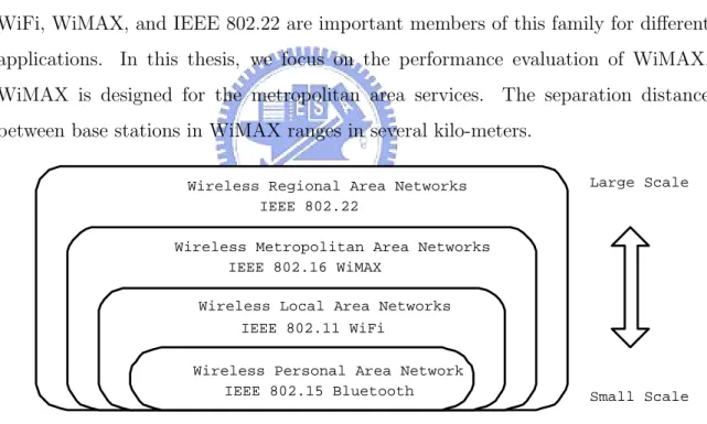
There are many IEEE standards for various wireless networks. In Fig. 2.1, Bluetooth, WiFi, WiMAX, and IEEE 802.22 are important members of this family for different applications. In this thesis, we focus on the performance evaluation of WiMAX. WiMAX is designed for the metropolitan area services. The separation distance between base stations in WiMAX ranges in several kilo-meters.

Wireless Regional Area Networks IEEE 802.22

Wireless Metropolitan Area Networks IEEE 802.16 WiMAX

Wireless Local Area Networks IEEE 802.11 WiFi

Wireless Personal Area Network

IEEE 802.15 Bluetooth _{Small Scale}

Large Scale

Figure 2.1: IEEE Wireless Networks

(20)

effi-are more complicated than OFDM. Hence, WiMAX is a promising solution to the last mile problem.

2.2 Downlink/Uplink in WiMAX

2.2.1 Downlink (DL)

WiMAX is an infrastructure-based network. There is a base station (BS) in a cell. The BS will broadcast preambles periodically to the mobile stations (MS). The preambles will help the MSs in BS recognition, frame detection, and signal synchronization. Frame control header (FCH) is next to the preamble and coding with predefined modulation coding scheme. MSs will read the FCH and get the information about this frame. The information includes: the DL/UL map, DL/UL channel descriptors, et, al. MSs can read the DL data according to the instructions in DL map.

2.2.2 Uplink (UL)

The UL part in a frame is followed behind the Time Transition Gap (TTG). Different MSs will have different TTGs in order to solve the near-far problem. Sending data to BS simultaneously by different MSs in different locations is achievable in OFDMA mode. MS must read and decode the UL map and send the data in the correct time and sub-channel which are assigned by BS. Different sub-channels will not share the same pilots in order to avoid the intra-cell interference.

(21)

2.3 OFDMA in IEEE 802.16

2.3.1 PHY Modes

IEEE 802.16 WiMAX supports four PHY modes. Single carrier is the original mode. The OFDM and OFDMA modes are usually used in recent applications. TDM can be applied in OFDM when the system need multiplexing. Hybrid of TDM and FDM can result in four OFDMA modes:

1) single carrier in 10-66 GHz;

2) single carrier a in sub-11 GHz with frequency domain equalization; 3) OFDM in sub-11 GHz with fixed FFT size (256);

4) OFDMA in sub-11 GHz with scalable FFT size (128, 512, 1024, and 2048).

2.3.2 OFDMA Air Interface and Frame Structure

In the OFDM mode, the data is transmitted by many orthogonal sub-carriers. The major merits of OFDMA include high efficiency of spectrum usage, simpler frequency domain equalizer, and resistance against the multi-path fading. Pilot tones are dis-tributed among the data carriers in order to estimate the channel. An overhead which called cyclic prefix (CP) is added in every OFDM symbol for synchronization to over-come the multi-path fading. The OFDMA is an extension version of OFDM, where sub-carriers are divided into groups, called sub-channels. Stations can use hybrid of FDM and TDM multiplexing.

The frame structure in OFDMA is shown in Fig. 2.2. An OFDMA symbol consists preamble, FCH, DL, and UL parts. The TTG is placed between DL and UL parts. It’s used for solving the near-far problem.

(22)

Prea mbl e Fra me Co ntr ol Heade r DL/UL Map DL User 1 DL User 2 DL User 4 DL User 5 DL User 3 UL User 1 UL User 2 UL User 3 UL User 4 Ranging Channel

Time

Subca

rr

ier

I

ndex

TTG

Frame n Frame n+1 Frame n+2 Frame n+3 Frame n+4 Frame n+5

Figure 2.2: A WiMAX OFDMA Symbol Sample

2.4 OFDMA in LTE

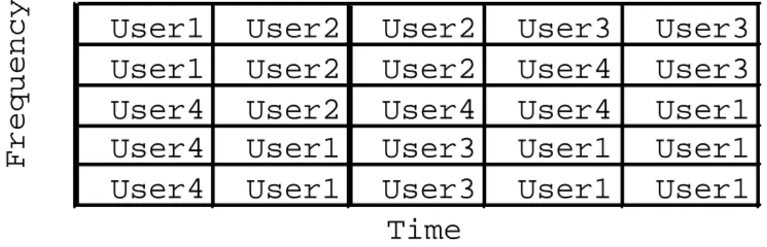
Long tern evolution (LTE) standard in the third generation partnership project (3GPP) is targeted on the market in the next ten years. The communication vendors may deploy the 4G networks using LTE technology as a foundation. LTE is a strong competitor for WiMAX. The goals of the uplink and downlink throughput of LTE are 50, 100 Mbps, respectively.

The OFDMA method will be applied for the physical-layer downlink trans-mission technique in the LTE system. The 3G systems use the CDMA modulation, but CDMA is not very suitable for the MIMO-based signal processing. OFDMA is a good modulation for MIMO signal processing. However, because of the severe peak to average power ratio (PAPR) problem, the FDMA is used instead of OFDMA in the uplink transmission for LTE. Another merit of FDMA is the power consumption is less than OFDMA. Power consumption is a severe problem for MSs. The minimum

(23)

resource block consists of 14 symbols and 12 sub-carriers. A sample of LTE OFDMA DL assignment is shown as Fig. 2.3.

User1 User2 User2 User3

User3

User1 User2 User2 User4

User3

User4 User2 User4 User4

User1

User4 User1 User3 User1

User1

User4 User1 User3 User1

User1

Time

Frequency

(24)

9

CHAPTER 3 Simulation Platform

3.1 Simulation Assumptions

The simulation assumptions consists of the parameters about BSs, MSs, and the prop-agation channel. In the realistic wireless channel, the signal will be deteriorated due to three reasons: path loss, shadowing, and fading. We will introduce the analytical models for each effect and consider thermal noise. With the bandwidth and the noise figure, we can estimate the received noise power.

The simulation scenarios are based on assumptions adopted by the IEEE 802.16 standards as shown in Table 3.1. Performance metrics considered in this thesis include the SINR, throughput, and fairness [15], [8], [14].

3.2 Path Loss Model

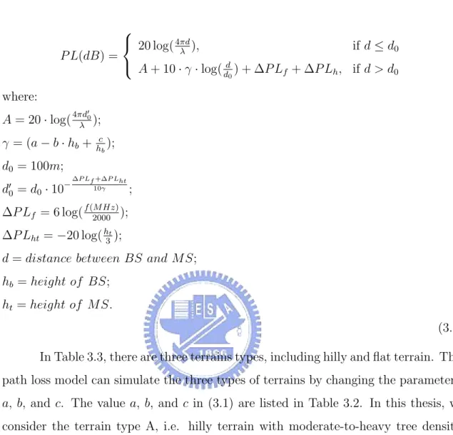
According to IEEE 802.16j evaluation methodology [9], path loss (P L) depends on distance d, carrier frequency f and antenna height. There are two regions of d. When

d ≤ d0, it is the line of sight (LOS) situation. P L only depends on d. On the other

hand, for d > d0, it is the non-LOS situation. We also consider f and antenna height.

(25)

Table 3.1: Simulation Assumptions

Parameter Value Parameter Value

Carrier Frequency 2.5 GHz Cell Structure Wrap Around 19 Cells

BS to BS Distance 1.732 Km Temperature 20o_C

Path Loss Model Sec 3.2 Shadowing Model Sec 3.3

Fading Channel Sec 3.4 Thermal Noise Sec 3.5

BS Height 32 m BS Tx Power 46 dBm

MS Height 1.5 m MS Tx Power 23 dBm

Scheduling Round Robin Antenna Pattern Sec 3.7

(26)

P L(dB) =    20 log(4πd λ ), if d ≤ d0 A + 10 · γ · log(d d0) + ∆P Lf + ∆P Lh, if d > d0 where: A = 20 · log(4πd00 λ ); γ = (a − b · hb+ _hc_b); d0 = 100m; d0 0 = d0· 10− ∆P Lf +∆P Lht 10γ ; ∆P Lf = 6 log(f (M Hz)₂₀₀₀ ); ∆P Lht = −20 log(h₃t);

d = distance between BS and MS;

hb = height of BS;

ht= height of MS.

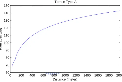
(3.1) In Table 3.3, there are three terrains types, including hilly and flat terrain. This path loss model can simulate the three types of terrains by changing the parameters: a, b, and c. The value a, b, and c in (3.1) are listed in Table 3.2. In this thesis, we consider the terrain type A, i.e. hilly terrain with moderate-to-heavy tree density. The effect of distance on path loss for terrian type A is shown in Fig. 3.1.

Table 3.2: Path Loss Parameters in Different Types of Terrains Model Parameter Terrain Type A Terrain Type B Terrain Type C

a 4.6 4 3.6

b 0.0075 0.0065 0.005

c 12.6 17.1 20

σµ 10.6 9.6 8.2

(27)

Table 3.3: Types of Terrains Terrain Type Description

A Hilly terrain with moderate-to-heavy tree density

B Intermediate path-loss condition

C Flat terrain with light tree densities

3.3 Shadowing Model

According to IEEE 802.16j evaluation methodology [9], shadowing is a log-normal random variable with standard deviation σ. Note that σ is related with distance d in (3.2).

σ(d) = σµ[1 − e−

|P L(d)−P Lfs(d)|

4 ] + 1.5, (3.2)

where: σµ is the maximum standard deviation; P L(d) is the mean path loss in dB;

P Lf s(d) is the free space path loss in dB.

Similar to pass loss, we consider the shadowing in LOS or NLOS based on the

distance. When d ¡ d0, LOS situation is considered. P L(d) is equal to P Lf s(d) and

the shadowing standard deviation is a constant 1.5. As d increases, σ(d) increases

(28)

0 200 400 600 800 1000 1200 1400 1600 1800 2000 60 70 80 90 100 110 120 130 140 150 Distance (meter) Path Loss (dB) Terrain Type A

Figure 3.1: Effect of Distance on Path Loss in the Terrain Type A of Propagation Model of IEEE 802.16 WiMAX

(29)

3.4 Frequency Selective Fading Channel

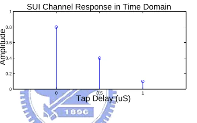
According to IEEE 802.16a contribution [6] ,the frequency selective fading channel

is described as three delayed taps in the time domain. The ith tap Ai is a Ricean

random variable in (3.3). After sampling and doing FFT, we can obtain the channel frequency response as:

Ai = R + M, (3.3)

where R is a Rayleigh random variable and M is the LOS component.

0 0.5 1 0 0.2 0.4 0.6 0.8 1

Tap Delay (uS)

Amplitude

SUI Channel Response in Time Domain

Figure 3.2: Time Domain Response of Stanford University Interim Channel Model (SUI)

(30)

100 200 300 400 500 600 700 800 900 1000 −8 −6 −4 −2 0 2 4 6 Sub−Carrier Index Gain (dB)

Figure 3.3: Frequency Domain Response of SUI-3 Model

(31)

3.5 Thermal Noise Budget

The thermal noise is considered as additive white gaussian noise (AWGN). The noise

power density N0 is proportional to absolute temperature T . That is:

N0 = K × T and K = 1.38 × 10−23 (m2kgs−2K−1) , (3.4)

where K is the Boltzman constant. The thermal noise desity in 20 o_{C is:}

10 log(1.38 × 10−23_{× (273 + 20)) + 30 = −173.9}dBm

Hz , (3.5)

Consider a bandwidth of 10MHz and the noise figures are 5 dB/ 7 dB in BS/ MS. The thermal noise power in MS will be:

−173.9 + 7 + 10 log(107_{) = −96.9dBm ,} _(3.6)

3.6 Wrap Around Scheme

In the IEEE 802.16m evaluation methodology [5], the wrap-around scheme is formed with 7 clusters and each cluster consists of 19 cells. In Fig. 3.4, only 19 cells in the middle are generated and the other interference cells are wrapped from the 19 cells. Each cell in the middle cluster can see two layers of interference sources. The merit of wrap around is to save the computation time and memory space in the simulation. The interference sources can be simulated correctly.

(32)

1

2

7

6

5

4

3

8

9

15

14

19

18

12

13

17

16

10

11

Figure 3.4: The 19 Cells in the Multi-Cellular System

3.7 Directional Antenna Pattern

In the IEEE 802.16m evaluation methodology [5], a cell will be divided into three sectors and the BS has three directional antenna, respectively. In this thesis, we will discuss three types of antenna patterns. The default antenna pattern is called the Wide-Beam Trisector Cell with Pentagon-Shaped Sector type. The other two types of directional antenna are Wide-Beam Trisector Cell with Diamond-Shaped Sector and Narrow-Beam Trisector Cell types, respectively.

(33)

3.8 Computation of per Sub-channel Effective SINR

The effective SINR in a sub-channel is related to the SINR in total sub-carriers. In [15], some metrics for SINR in the multi-carrier case are introduced, such as expo-nentially effective SINR map (EESM), effective code rate map (ECRM), and mean instantaneous capacity (MIC).

In this thesis, we adopt the MIC method. Denote γ the effective SINR in a

sub-channel, and γi the SINR in a sub-carrier. Based on the Shannon’s information

capacity rule, the capacity of a sub-channel is the summation of the capacity of the sub-carriers. Let Ns be the number of sub-carriers in a sub-channel. Then we can have: log₂(γ + 1) = N s X i=1 1 Nslog2(γi + 1) , (3.7) γ = 2N s1 PN s i=1log2(γi+1)_{− 1 ,} _(3.8)

3.9 Capacity Evaluation

Fig. 3.5 shows the link level throughput v.s. SINR for the IEEE 802.16 OFDM mode with seven adaptive modulation coding schemes (MCS) [8]. The evaluation is based on OFDM FFT size of 256 and 3.5 MHz bandwidth. The capacity can be obtained from SINR and linear interpolation. PHY parameters used in this thesis and in [8]

(34)

Table 3.4: PHY Parameters in This Thesis and in [8]

Parameters Bandwidth FFT Size Number of Sub-channel

This Thesis 10 MHz 1024 30

[8] 3.5 MHz 256 1

Figure 3.5: Effect of Various SINR on the Throughput with Different Modulation and Coding Schemes

(35)

3.10 Fairness Index

Fairness is an important issue. If the system is on fair, the poor-throughput users will be very unconformable and may exist the network and join another network soon. It’s not a good idea if the network provider want to develop their business.

According to [14], we use the Jain’s fairness index to evaluate the fairness

among the users in the cell. The fairness index (F I) among variables x1,x2,...,xn is

defined as (3.9). The (F I) is related to the the first moment and second moment.

F I(x1, x2, ..., xn) = (Σn i=1xi)2 nΣn i=1x2i , (3.9)

The properties of (F I) are: 1. 0 ≤ F I ≤ 1;

2. F I= 1 when all the xi are the same;

3. Larger F I implies fairer.

For example, if all the xi are the same, i.e. xi = 1, this is the fairest situation.

(F I) is one, i.e. F I(x1, x2, ..., xn) = (Σn i=11)2 nΣn i=112 = n2 n × n = 1 , (3.10)

(36)

21

CHAPTER 4 Effects of the Interference Averaging

Technique: Sub-carrier Permutation

4.1 Types of Sub-carrier Permutation

Permutation is the way to allocate the sub-carriers in a sub-channel. There are two types of permutations: Continuous sub-carrier and randomly distributed sub-carrier permutation methods, as shown in Table 4.1. The usage of sub-channel can save the size of the header in MAC layer. For a 1024-point FFT, we need 10 bits to allocate a carrier. For a 64-QAM modulation, there are only 6 information bits in a sub-carrier. The huge size for indexing sub-carriers is not practical. For a sub-channel with 48 sub-carriers, one can only use 5 bits to index the total 30 sub-channels.

In the IEEE 802.16m evaluation methodology [5], the PUSC permutation is suggested. PUSC is used together with the Wide-Beam Trisector Cell with Pentagon-Shaped Sector antenna pattern. We will discuss the details of the antenna pattern in Chapter 6. There are six major groups and each group has its own pilots. BS sends only two major groups into the air from each sector. For comparison, Band AMC is also discussed as the adjacent type permutation.

(37)

Table 4.1: Permutation Types in WiMAX Sub-Carrier Permutation Type Example

Randomly Distributed

PUSC (Partial Usage of the Sub-Channels) OPUSC (Optional PUSC)

FUSC (Full Usage of the Sub-Channels) OFUSC (Optional FUSC)

Continuous Band AMC (Band Adaptive Modulation and Coding)

FUSC is suitable for the broadcast messages since FUSC uses the whole band of bandwidth. The pilots are common among all the sub-channels. All the sectors must sent all the sub-carriers and pilots into the air. Usually FUSC is used with omni-directional antenna. We will discuss the FUSC in Chapter 6, which is omniomni-directional antenna and suitable in broadcast situations.

4.2 Down Link PUSC

4.2.1 Symbol Structure

In the IEEE 802.16e standard [10], an OFDMA PUSC symbol contains guard sub-carriers, dc carrier, and clusters. The symbol structure is shown as Fig. 4.1. The frequency of dc carrier is the same as carrier frequency. We can’t transmit data at dc carrier. The guard sub-carrier is designed to avoid the leakage from the adjacent frequency bands. There are 60 clusters and 720 data carriers in an OFDMA symbol.

(38)

92 Guard Sub-carriers 91 Guard Sub-carriers DC Cluster 0 Cluster 1 Cluster 29 Cluster 30 Cluster 59

60 Clusters of 14 Adjacent Sub-carriers Each

1024-FFT OFDMA Symbol

Figure 4.1: PUSC Symbol Structure

Time Sub-Carrier Index Data Carrier Pilot Carrier

Even OFDMA Symbols

Odd OFDMA Symbols P

P P

P

Figure 4.2: PUSC Cluster Structure

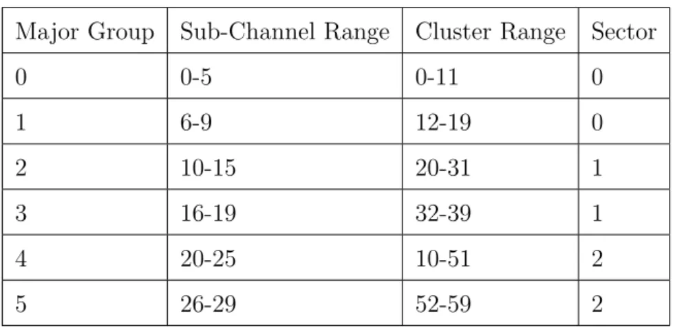
symbols. The cluster structure is shown as Fig. 4.2. This is helpful in synchronization because ofthe regular structure of the pilots. It’s good for channel estimation since we can learn four pilots in a cluster. In Table 4.2, 30 sub-channels can be divided into 6 major groups. Two groups are used in each sector. The sub-channels in one major group corresponded to on specific set of clusters.

4.2.2 Renumbering and Permutation Base Assignment

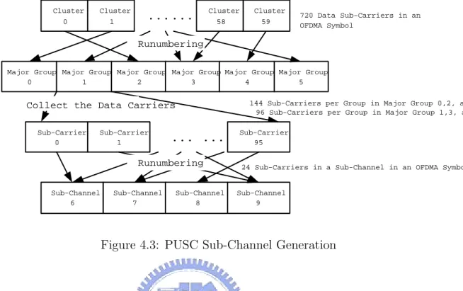
During the PUSC channel assignment, the renumbering occurs twice.T Renumbering is depended on the parameter: permutation base. For example, in Fig. 4.3 there are 60 clusters in an OFDMA PUSC symbol. The clusters will be renumbered and collected into 6 major groups. In Major Group 1, there are 96 data sub-carriers after removing the pilots. Now we do the renumbering and collection again. The 96 sub-carriers will be renumbered and collected into 4 sub-channels.

(39)

Table 4.2: PUSC Sub-Channels

Major Group Sub-Channel Range Cluster Range Sector

0 0-5 0-11 0 1 6-9 12-19 0 2 10-15 20-31 1 3 16-19 32-39 1 4 20-25 10-51 2 5 26-29 52-59 2

DL PermBase is an integer ranging from 0 to 31, which can be indicated by down-link map (DL MAP) for PUSC. It’s used in distributing the clusters and sub-carriers. The cluster number will be renumbered based on DL PermBase. In (4.1), the actually index in hardware is the physical number.

Cluster Logic N umber = Renumbering Sequence

((Cluster P hysical Number + 13 · DL P ermBase) mod Nclusters) (4.1)

We define two types of permutation usage as shown in Table 4.3. In type 0, various BSs can use the same permutation base. In type 1, permutation bases are different among various cells.

(40)

Cluster 0 Cluster 1 Cluster 59 Cluster 58 ... Major Group 0 Major Group 1 Major Group 5 Sub-Carrier 0 Sub-Carrier 1 ... Sub-Carrier 95 Sub-Channel 6 Sub-Channel 7 Sub-Channel 8 Sub-Channel 9 Runumbering

Collect the Data Carriers

Runumbering Major Group 4 Major Group 3 Major Group 2 720 Data Sub-Carriers in an OFDMA Symbol

144 Sub-Carriers per Group in Major Group 0,2, and 4 96 Sub-Carriers per Group in Major Group 1,3, and 5

24 Sub-Carriers in a Sub-Channel in an OFDMA Symbol

Figure 4.3: PUSC Sub-Channel Generation

Table 4.3: Permutation Base

Assignment Type Permutation Base Value Among Different Cells

Type 0 Same

Type 1 Random

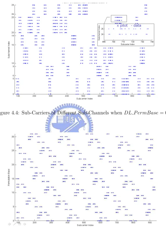
4.2.3 Results of Locations of Sub-carriers in PUSC

Fig. 4.4 shows the sub-carriers for different sub-channels when DL P ermBase = 0 in (4.1). We can see that the six major groups can be separated in frequency domain. Fig. 4.5 shows the effects of different Permutation Base. We can see that the frequency segment can be done in PUSC Type 0. However, the frequency segmentation is not achievable when the Permutation Base is different even though we use the same 7th sub-channels in different cells.

(41)

(42)

4.3 Down Link FUSC Permutation

FUSC is another important member of randomly distributed sub-carrier permutation method. A FUSC symbol is constructed using guard carriers, pilots, data carriers, and the DC carrier. In a 1024-FFT OFDMA symbol, there are 768 data carriers and 82 pilots. All the pilots and data carriers are distributed in the whole frequency band. It’s suitable for omnidirectional antenna. The symbol structure of FUSC is shown in Fig 4.6. 87 Guard Carriers 86 Guard Carriers DC Carrier 82 Pilots ... ... ... ... ... 768 Data Carriers Sub-Carrier 0 Sub-Carrier 1 Sub-Carrier 765 Sub-Carrier 764

Collect the Data Carriers

... ... ... ... ... Sub-Channel 0 Sub-Channel 1 Sub-Channel 14 Sub-Channel 15 ... Sub-Channel ... ... 7 Sub-Channel 8 ...

Figure 4.6: FUSC Symbol structure and Sub-Channel Generation

4.4 Down Link Band AMC Permutation

Similar to PUSC, an OFDMA Band AMC symbol contains guard sub-carriers, dc carrier, and bins. A bin contains 8 data carriers and 1 pilot carrier. In 1024-FFT mode, there are 96 bins in an OFDMA symbol. The structure of a bin and Band AMC sub-channel is shown in Fig. 4.7.

(43)

There are 4 types in Band AMC. Each type occupies different OFDMA symbol number and consecutive bins in the same time. Table 4.4 shows the details. If the coherence time of the channel is long enough, we can choose the Band AMC type in larger OFDMA symbols.

B B B B B B

OFDMA Symbol Number (Time)

Bin

Inde

x

(Fr

eque

ncy)

B B B B B B B B B B B B B B B B B B

Type 1

Type 2

Type 3

Type 4

Data Data Data Data Data Data Data Data Pilot

Figure 4.7: Band AMC Bin and Sub-Channel Structure Table 4.4: Band AMC Sub-Channels

Type Bins and Symbols Sub-channels

Type 1 6 bins × 1 OFDMA symbol 16

Type 2 2 bins × 3 OFDMA symbols 48

Type 3 3 bins × 2 OFDMA symbols 32

Type 4 1 bin × 6 OFDMA symbols 96

(44)

4.5 Numerical Results

In this section, we concern about the cumulative distribution function (CDF) of users’ received SINR. We focus on the 90% tile because it implies the quality of the poor users in the system. The users who get poor throughput usually complain and need help. The CDF is shown in Fig. 4.8

The traffic load is defined as the load of the adjacency cells. In this thesis, we close some proportion of sub-channels to simulate the traffic load. This is because that we don’t simulate the MAC layer. Table 4.5 and Fig. 4.9 show the results the 90% tile of users. −20−19−18−17−16−15−14−13−12−11−10 −9 −8 −7 −6 −5 −4 −3 −2 −10 0 1 2 3 4 5 6 7 8 9 10 0.05 0.1 0.15 0.2 0.25 0.3 SINR (dB)

Probability of The Uer’s SINR > Abscissa

TL=0.2 BandAMC TL=1.0 BandAMC TL=0.2 PUSC Type 0 TL=1.0 PUSC Type 0 TL=0.2 PUSC Type 1 TL=1.0 PUSC Type 1

Figure 4.8: The Users’ SINR in PUSC Type 0, PUSC Type 1, and Band AMC

(45)

Table 4.5: The 90% Tile of Users’ Received SINR for Fig. 4.8 Type TL=0.2 TL=0.6 TL=1.0 PUSC Type 0 0.7135 -7.4572 -11.1309 PUSC Type 1 6.2728 -1.7477 -5.7498 Band AMC -1.1269 -9.9525 -13.7623 0 0.1 0.2 0.3 0.4 0.5 0.6 0.7 0.8 0.9 1 −14 −12 −10 −8 −6 −4 −2 0 2 4 6

Traffic Load of Adjacent Cells

The 90% Tile of Users’ Received SINR

PUSC Type 1 PUSC Type 0 Band AMC

Figure 4.9: The 90% Tile of Users’ Received SINR Figure

4.5.1 Comparison of PUSC and Band AMC

(46)

further. We can say that the PUSC get the merit from the frequency selective fading channel. PUSC Type 0 needs the additional cooperation among cells but gets poorer performance than PUSC Type 1. It’s not suggested in this thesis.

4.5.2 Comparison of Distributed or Contiguous Sub-Carriers

Fig. 4.10 shows how the distributed permutation can ease the co-channel interference. In distributed method PUSC, only some sub-carrier will suffer co-channel interference, and the signal may be recovered by some coding methods. However, in contiguous permutation Band AMC, if there is an interference source nearby, all the sub-carriers will suffer severe co-channel interference.

0 100 200 300 400 500 600 700 800 900 1000

PUSC Signal PUSC Interference Band AMC Signal Band AMC Interference

0 2 4 6 Subcarrier Index Channel Response

Figure 4.10: Comparison of Randomly Distributed and Contiguous Subcarrier Per-mutations

(47)

32

CHAPTER 5 Effects of the Interference Avoidance

Technique: Frequency Reuse

5.1 Types of Frequency Reuse

5.1.1 Regular Frequency Reuse

The frequency reuse can change the distance of co-channel interference source from the other cell. The larger distance induces smaller interference. The concept of reuse was proposed in 1979 [11]. The reuse factor N can be obtained from (5.1) and (5.2). The total bandwidth W is divided into N parts, and the available bandwidth of each

user is W

N.

N = i2_{+ ij + j}2 _(5.1)

where i, j are non-negative integers.

(48)

In this thesis, we would like to evaluate the N= 1, 3, 4, and 7. Fig. 5.1 illustrates the locations of interference cells related to the center cell when N= 3, 4, and 7. The basic unit is the cell, and cells with the same index number use the same frequency band. N cells is combined as a cluster, and the available frequency band of these cells will not be duplicate. Hence, there is no intra-cluster interference within a cluster. 1 3 2 1 3 2 1 3 2 1 3 2 1 3 2 1 3 2 1 3 2 1 4 3 2 1 4 3 2 1 4 3 2 1 4 3 2 1 4 3 2 1 4 3 2 1 4 3 2 5 6 1 4 7 3 2 5 6 1 4 7 3 2 5 6 1 4 7 3 2 5 6 1 4 7 3 2 5 6 1 4 7 3 2 5 6 1 4 7 3 2 5 6 1 4 7 3 2

Figure 5.1: Cell Planning when Reuse Factor N= 3, 4, and 7

(49)

5.1.2 Fractional Frequency Reuse

In [12], the fractional frequency reuse (FFR) can be applied in the WiMAX systems. A cell will be divided into two parts: inner circle and outer ring. Fig. 5.2 illustrates an example of FFR scheme with 3 cells. The users in outer ring in each cell use frequency: F 1, F 2, and F 3, respectively, and the users in inner circle use the frequency band F 0.

Comparing to reuse factor N= 1, i.e. there is no outer ring in the system, the FFR will induce: 1) The co-channel interference of the outer users can be reduced; 2) The usable bandwidth is less. We will discuss the two effects in this thesis.

F1

F2

F3

F0

(50)

5.1.3 Achievable FFR Factors

We assume that the reuse factor N in inner circle is not smaller than the reuse factor N in the outer ring. The achievable FFR schemes in this thesis are listed in Table 5.1. The ratio p is defined as (5.3).

p = Number of Channels in Outer Ring

Number of Channels in Outer Ring and Inner Circle (5.3)

The FFR factor is calculated in (5.4). In this thesis, we will choose some values from Table 5.1. The reuse factor is:

Reuse F actor = Number of Channels

Number of Assigned Channels per Cell (5.4)

Reuse F actor = p × RFOuter Ring+ (1 − p) × RFInnerCircle (5.5)

For example, if p = 3

8, RFinner = 1, and RFouter = 3, we can assume that the

number of assigned channels per cell is 8. The number of channels in inner circle/outer ring are 3/5. The total number of channels in the system is 3×3+5×1 = 14. Finally,

the reuse factor is 14

8 = 134.

5.2 Inner Circle and Outer Ring User Decision

In Section 5.1.2, the shape of the inner circle is a round shape. However, the round shape is not reasonable in this thesis because of the antenna gain, cell structure, and

(51)

Table 5.1: FFR Values

RF Inner Circle RF Outer Ring p = 1

8 p = 38 p = 48 p = 58 p = 68 1 1 1 1 3 11 4 134 2 214 1 4 13 8 218 212 278 1 7 31 4 4 4 3 4 3 3 3 3 4 33 8 312 358 3 7 41 2 5 512 6 4 4 4 4 7 51 8 512 578 614 7 7 7

shadowing in the simulation platform of this thesis. Instead, the decision of that the user is in inner circle or outer ring is based on the signal strength of the user. In Fig. 5.4, 20 users are divided into 10 inner users and 10 outer users by their signal strength.

The signal strength is a basic parameter in wireless cellular systems. Fig. 5.3 shows a sample of signal strength in a 2G system. In the IEEE 802.16, the BS and MS can get the signal strength from ranging messages. Signal strength based decision is more reasonable than distance based decision in this thesis. If we use the distance in decision, the received power of users of inner circle and outer ring are not the same due to the directional antenna. Another reason is that it’s hard for BS to measure

(52)

Signal

Strength

Figure 5.3: Signal Strength in a 2G System Cell Phone

Original User Index Inner Users Outer Users 0 10 20 30 40 50 60 70 80 90 100 Sorting =>

Figure 5.4: Selection of Inner and Outer Users by Sorting on Received Power Strengths

(53)

5.3 Permutation Base Assignment in Frequency

Reuse

Similar to Chapter 4, the assignment of the Permutation Base will affect the system performance under FR planning. Compared to Table 4.3, the cluster is a new consid-eration in Table 5.2. Fig. 5.5 shows the difference between PUSC Type 0 and Type 1 when RF= 3. In order to divide the frequency band into partitions, Permutation Base in a cluster must be the same otherwise the intra-cluster interference can not be avoided. In PUSC Type 0, the users suffer interference only from one cell from the adjacent cluster. In PUSC Type 1, the users suffer interference from all the cells from the adjacent clusters, but the strength of the interference from each cell is less than that in PUSC Type 0.

1 3 2 1 3 2 1 3 2 1 3 2 1 3 2 1 3 2 1 3 2 Type 0 1 3 2 1 3 2 Type 1 1 3 2 1 3 2 1 3 2 1 3 2 1 3 2

(54)

Table 5.2: Permutation Base Assignment with Frequency Reuse Assignment Type Permutation Base Among Different Clusters

Type 0 Same

Type 1 Random

5.4 Relation of Frequency Reuse and Throughput

Fig. 5.6 shows the trends of reuse factor and throughput. In this thesis, the power of interference strongly depends on the distance with path loss exponent γ. By (5.2), we get the relationship between SINR and N in (5.6). The SINR is increasing as reuse factor increasing. In Siemens [8], users can use the adaptive MCS in various SINRs. This means the higher SINR, users can get higher throughput.

However, the usable channels of users will shrink as reuse factor increasing in (5.7). This is because the usable bandwidth will be divided into some parts. There are trade-offs between these two effects. We will see these two parts in the numerical results.

SIN R ∝ 1

Interf erence P ower ∝ (R

√

3N)γ _{∝ N}γ₂ _(5.6)

Usable Channel ∝ N−1 (5.7)

(55)

Reuse Factor User Rx SINR Usable Channels MCS Throughput Throughput Throughput ?

Figure 5.6: Trends of Reuse Factor and Throughput (↑ Increasing, ↓ Decreasing)

5.5 Numerical Results

5.5.1 Effects of FFR on SINR

Fig. 5.7 shows the effects of the trend as FFR increasing in PUSC Type 0, PUSC Type 1 and Band AMC respectively. The PUSC Type 1 gets the best performance among the three types. The PUSC Type 0 is better than the Band AMC. We can see that as the reuse factor increasing, the users will get higher SINR. The differences of SINR curve are larger when reuse factor is one to three. As the reuse factor increasing, the differences among the curves are smaller.

We also figure out the SINR in FUSC permutation with omnidirectional an-tenna in Fig. 5.8. We will compare the performance on directional and omnidirec-tional antenna patterns in Chapter 6.

5.5.2 Effects of FFR on Link Quality

In Fig. 5.9, the 90% tile of users’ received SINR will higher as the reuse factor increasing. However, the improvement is not obvious when reuse factor is greater than three. The largest improvement of link quality occurs when the reuse factor is

(56)

−30 −20 −10 0 10 20 30 40 10−2 10−1 100 PUSC Type 0 SINR

Probability of User’s SINR > Abscissa

RF=1 RF=1.25 RF=1.75 RF=2 RF=3 RF=7 −30 −20 −10 0 10 20 30 40 10−2 10−1 100 PUSC Type 1 SINR

RF=1 RF=1.25 RF=1.75 RF=2 RF=3 RF=7 −30 −20 −10 0 10 20 30 40 10−2 10−1 100 Band AMC SINR

RF=1 RF=1.25 RF=1.75 RF=2 RF=3 RF=7

Figure 5.7: CDF of SINR in PUSC Type 0 and Type 1, Band AMC with Varies Reuse Factor in Interference Traffic Load= 100%

(57)

−30 −20 −10 0 10 20 30 40 10−2 10−1 100 FUSC Type0 SINR

RF=1 RF=1.25 RF=1.75 RF=2 RF=3 RF=7 −30 −20 −10 0 10 20 30 40 10−2 10−1 100 FUSC Type1 SINR

RF=1 RF=1.25 RF=1.75 RF=2 RF=3 RF=7

Figure 5.8: CDF of SINR in FUSC Type 0 and Type 1 with Varies Reuse Factor in Interference Traffic Load= 100%

1 2 3 4 5 6 7 −15 −10 −5 0 5 10 15 20

The 90% Tile of Users’ Received SINR

TL=0.2 PUSC Type0 TL=0.2 PUSC Type1 TL=0.2 Band AMC TL=1.0 PUSC Type0 TL=1.0 PUSC Type1 TL=1.0 Band AMC

(58)

5.5.3 Effects of FFR on Throughput

The reuse factor affects the usable channels and SINR of users. In Fig. 5.6, system throughput may be increasing or decreasing as the reuse factor increasing.

In Fig. 5.10, we can say that the usage of frequency reuse is not useful for the cell total throughput. The decreasing usable channels is the dominate affection in the system. The merit of higher SINR and better MCS does not compensate for loss of throughput due to loss of usable frequency bands.

1 2 3 4 5 6 7 2 4 6 8 10 12 14 Reuse Factor

Data Rate (MBit/Sec)

PUSC Type 0 PUSC Type 1 Band AMC Inference Traffic Load=0.2

Inference Traffic Load=0.6

Inference Traffic Load=1.0

Figure 5.10: Reuse Factor and Cell Capacity

5.5.4 Effects of FFR on Inner Circle and Outer Ring Users

Fig. 5.11 shows the throughput of users in inner circle and outer ring under PUSC Type 1, and Fig. 5.12 shows the fairness of the total users. We can see that the throughput of inner users is the best when reuse factor N is one. The outer user

(59)

will suffer poor SINR channels in higher traffic loads (0.6 and 1.0). The sub-carrier permutation is not very powerful for the outer users in these scheme.

However, the outer users get better SINR when reuse factor N is two. Com-pared to the case N= 1, the improvements are about 7% to 40%. When reuse factor N is greater than three, the throughput of inner/outer users shrinks as reuse factor N increasing. The fairness is increasing but the improvement is saturated in high reuse factor N. It’s not suggested in the environment in this thesis.

In low traffic load (0.2), the SINR is high enough for outer users. So the reuse factor is not very helpful when reuse factor N is greater than 1. There is a large improvement of fairness when N is one to two. The fairness improves as N >3 but the improvement is saturated.

1 1.2 1.4 1.6 1.8 2 1.4 1.6 1.8 2 2.2 2.4 2.6 2.8 Reuse Factor 40% 7% 1 2 3 4 5 6 7 1 2 3 4 5 6 7 8 Reuse Factor

TL=0.2 Inner Users TL=0.6 Inner Users TL=1.0 Inner Users TL=0.2 Outer Users TL=0.6 Outer Users TL=1.0 Outer Users

(60)

1 2 3 4 5 6 7 0.65 0.7 0.75 0.8 0.85 0.9 0.95 1 Reuse Factor Fairness Index TL=0.2 TL=0.6 TL=1.0

Figure 5.12: The Fairness Index of the Users’ Throughput in PUSC Type 1

5.5.5 Comparison of PUSC Type 0 and 1

The distributions of interference sources of PUSC Type 0 and 1 are different. In order to verify the difference, we locate three test users A, B, and C and check the power of interference sources from PUSC Type 0 or 1. The location of users A, B, and C are shown in the left side of Fig. 5.13.

Since some sources of co-channel interference are closer in PUSC Type 1 than in PUSC Type 0, but more sources are further. The result is that the interference power is smaller in PUSC Type 1 in the right side of Fig. 5.13. The performance of PUSC Type 1 will be better than PUSC Type 0 in this thesis.

(61)

1 3 2 1 3 2 1 3 2 1 3 2 1 3 2 1 3 2 1 3 2 A B C 151 152 153 154 155 156 157 158

User A User B User C

Path Loss for Total Interference Sources (dB))

PUSC Type 0 PUSC Type 1

(62)

47

CHAPTER 6 Effects of the Interference Mitigation

Technique: Directional Antenna

6.1 Types of Directional Antenna

In this chapter, we’d like to verify different types of directional antennas and the omnidirectional antenna in the multi-cell system. Both in [5] and [7], different antenna patterns are introduced. Three types of antenna patterns involved in this thesis are shown as Table 6.1. [5] suggests the Wide-Beam Trisector Cell with Pentagon-Shaped (WBTC) with type. Wide-Beam Trisector Cell with Diamond-Shaped Sector and Narrow-Beam Trisector Cell (NBTC) types are mentioned by [7].

Table 6.1: The Three Directional Antennas

Antenna Pattern Source Cited

Wide-Beam Trisector Cell with Diamond-Shaped Sector [7]

Narrow-Beam Trisector Cell [7]

(63)

−150 −100 −50 0 50 100 150 −60 −50 −40 −30 −20 −10 0 10 20 Angle (Degree) Antenna Gain (dB) NBTC

WBTC with Diamond−Shaped Sector WBTC with Pentagon−Shaped Sector

Figure 6.1: Antenna Gain

The gains of the three directional antenna patterns are shown Fig. 6.1. The

main-lobe is located in 0o_{and the gain angle is ranging in -180}o _{to 180}o_{. There is some}

small amount of leakage in the side-lope. The front-to-end power ratio is constant in the WBTC with Pentagon-Shaped Sector pattern.

In the multi-cell environment, we use “BS-to-BS distance” instead of “cell coverage” in this thesis since the cell architectures are not circular. For comparison, the BS-to-BS distance among the three systems will be the same. So the density of BS is the same. In Fig. 6.2 we can see the adjacent cells multi-cell environment under the same BS density.

(64)

BS BS BS BS BS BS BS

WBTC with

Diamond-Shaped Sector

NBTC

WBTC with

Pentagon-Shaped Sector

Figure 6.2: The Three Antenna Patterns in Multi-Cellular Environment

(65)

WBTC with Diamond−Shaped Sector

Distance: 970 m Path Loss: 128 dB Antenna Gain: 14 dB Distance: 865 m Path Loss: 125 dB Antenna Gain: 11 dB Distance: 1000 m Path Loss: 129 dB Antenna Gain: 15 dB

Figure 6.3: WBTC with Diamond-Shaped Sector Antenna Pattern and Cell Boundary

6.1.1 WBTC with Diamond-Shaped Sector

WBTC with Diamond-Shaped Sector antenna uses a 120o _{antenna pattern in each}

sector. The shapes of the sectors are diamonds and form the cell structure as a hexagon. It’s most conventional for multi-cellularsystems.

(66)

NBTC

Distance: 870 m Path Loss: 126 dB Antenna Gain: 15 dB Distance: 568 m Path Loss: 117 dB Antenna Gain: 6 dB Distance: 1000 m Path Loss: 129 dB Antenna Gain: 18 dB

Figure 6.4: NBTC Antenna Pattern and Cell Boundary

6.1.2 NBTC

NBTC uses a 60o _{antenna in each sector. The shape of the sector is a hexagon. Three}

antennas form the cell structure as a clover leaf. The energy leakage in the side-lobe is smaller than WBTC type.

(67)

WBTC with Pentagon−Shaped Sector Coverage Hole Distance: 567 m Path Loss: 117 dB Antenna Gain: 9 dB Distance: 779 m Path Loss: 123 dB Antenna Gain: 15 dB Distance: 886 m Path Loss: 125 dB Antenna Gain: 17 dB

Figure 6.5: WBTC with Pentagon-Shaped Sector Antenna Pattern and Cell Boundary

6.1.3 WBTC with Pentagon-Shaped Sector

WBTC with Pentagon-Shaped Sector antenna pattern uses an 120o _{antenna pattern}

as that in WBTC with Diamond-Shaped Sector antenna pattern. There is 30o_-angle

rotation between them. The antenna pattern is specified as (6.1). As shown in Fig. 6.1, the coverage hole in the cell boundary is larger than the other two antenna types.

A(θ) = − min[12( θ

θ3dB

)2_{, A}

(68)

200 300 400 500 600 700 800 900 Sub−carrier Index

Data Carrier Pilot Carrier

Figure 6.6: The Sub-Channels and Pilots in FUSC Permutation

Omnidirectional Antenna

Distance: 1000 m Path Loss: 129 dB Antenna Gain: 0dB

Figure 6.7: Omnidirectional Antenna Pattern and Cell Boundary

6.2 Omnidirectional Antenna and FUSC

For comparison, we also consider the omnidirectional antenna in this system. The antenna gain in omnidirectional antenna system is assumed 0 dB in each direction. The sub-carriers in FUSC spread in the whole band, so FUSC is suitable in omnidi-rectional antenna application and broadcast purpose. Fig. 6.6 shows the locations of the 16 sub-channels and pilots in FUSC permutation. The cell structure is a hexagon and the antenna pattern is a round shape in Fig 6.7.

(69)

1 1.2 1.4 1.6 1.8 2 6 7 8 9 10 11 12 13 Reuse Factor

0.5 0.6 0.9 0.3 0.4 0.2 1 2 3 4 5 6 7 2 4 6 8 10 12 14 Reuse Factor

NBTC TL=0.2

WBTC with Diamond−Shaped Sector TL=0.2 WBTC with Pentagon−Shaped Sector TL=0.2 NBTC TL=0.6

WBTC with Diamond−Shaped Sector TL=1.0 WBTC with Pentagon−Shaped Sector TL=1.0

Figure 6.8: Cell Capacity in Three Different Directional Antennas

6.3 Numerical Results

6.3.1 Effect on Throughput

The system capacity will decrease as reuse factor N increases. The NBTC type is the best type in terms of throughput as shown in Fig. 6.8. The NBTC gets more 0.2 to 0.9 Mbps throughput when reuse factor is about 1 or 2. The capacity of WBTC with Diamond-Shaped Sector and WBTC with Pentagon-Shaped are similar. This is because the cell structures of WBTC with Diamond-Shaped Sector and WBTC with Pentagon-Shaped Sector are similar. Both of them are hexagon structure.

(70)

1 2 3 4 5 6 7 2 4 6 8 10 12 14 Reuse Factor

NBTC TL=0.2

WBTC with Diamond−Shaped Sector TL=1.0 WBTC with Pentagon−Shaped Sector TL=1.0 Omnidirectional Antenna TL=0.2 Omnidirectional Antenna TL=1.0 34 % 30 % 24 % 52 % 55 % 35 %

Figure 6.9: Cell Capacity in Directional and Omnidirectional Antennas

The gain between directional and omnidirectional antenna patterns are larger. In Fig. 6.9, the cells with the directional antennas get more 24% to 55% capacity than omnidirectional antenna systems. In high traffic load, the improvements are larger.

6.3.2 Effect on Link Quality

The 90% tile of users’ received SINR is shown in Fig. 6.10. The omnidirectional antenna system gets less 9.6 to 13.8 dB link quality than the directional antenna sys-tems. This is because the co-channel interference in omnidirectional systems is higher

(71)

1 2 3 4 5 6 7 −10 −5 0 5 10 15 20 Reuse Factor

The 90% Tile of the Users’ Received SINR

NBTC TL=0.2

WBTC with Diamond−Shaped Sector TL=1.0 WBTC with Pentagon−Shaped Sector TL=1.0 Omnidirectional Antenna TL=0.2 Omnidirectional Antenna TL=1.0 11.1 10.2 13.8 9.4 1.1 1.2 0.9 1.6 0.6 0.4 1.4 0.3

Figure 6.10: The 90% tile of Users’ Received SINR in Different Antennas

than that in directional antenna systems. The link quality of the NBTC antenna pat-tern is the best. The WBTC with Pentagon-Shaped gets the worst performance in the three directional antennas. The NBTC can get more 0.6 to 1.4 dB link quality than the other two directional antenna. The largest improvement of the link quality is in the range when reuse factor is about one or two.

6.3.3 Effect on the Capacity and Fairness of Inner/Outer

Users

(72)

when antenna pattern changes.

For outer users, there are larger improvements in NBTC type. In high in-terference traffic load, there are good improvements when reuse factor is about two. Outer users’ capacity can be boosted by 15 % to 24 %. The improvements are larger in WBTC with Diamond-Shaped Sector and WBTC with Pentagon-Shaped types. Because of the better performance of outer users, NBTC is the fairest type of the three types. 1 2 3 4 5 6 7 1 2 3 4 5 6 7 8 Reuse Factor

NBTC TL=0.2

Figure 6.11: Inner Users’ Throughput in Three Different Directional Antennas

(73)

1 1.2 1.4 1.6 1.8 2 2 2.1 2.2 2.3 2.4 2.5 2.6 2.7 2.8 2.9

15%

24%

1 2 3 4 5 6 7 1 1.5 2 2.5 3 3.5 4 4.5 5 5.5 6 6.5 Reuse Factor

NBTC TL=0.2

(74)

1 2 3 4 5 6 7 1 2 3 4 5 6 7 8 Reuse Factor

Inner Users

NBTC TL=0.2

WBTC with Diamond−Shaped Sector TL=1.0 WBTC with Pentagon−Shaped Sector TL=1.0 Omnidirectional Antenna TL=0.2 Omnidirectional Antenna TL=1.0 7% 0.66 MBit/Sec 35% 1.79 MBit/Sec

Figure 6.13: Inner Users’ Throughput in Directional and Omnidirectional Antennas

The usage of directional antenna gives lots of help for the outer users. In Fig. 6.13 and 6.14, we can see the inner/outer users get more throughput than in omnidirectional antenna systems. The outer users get more merits from directional antennas.

(75)

1 2 3 4 5 6 7 0 1 2 3 4 5 6 Reuse Factor

Outer Users

NBTC TL=0.2

WBTC with Diamond−Shaped Sector TL=1.0 WBTC with Pentagon−Shaped Sector TL=1.0 Omnidirectional Antenna TL=0.2 Omnidirectional Antenna TL=1.0 105% 3.15 MBit/Sec 225% 1.71 MBit/Sec

(76)

1 2 3 4 5 6 7 0.5 0.55 0.6 0.65 0.7 0.75 0.8 0.85 0.9 0.95 1 Reuse Factor Fairness Index _{NBTC TL=0.2}

WBTC with Diamond−Shaped Sector TL=1.0 WBTC with Pentagon−Shaped Sector TL=1.0 Omnidirectional Antenna TL=0.2 Omnidirectional Antenna TL=1.0 0.03 0.01 0.05 0.03 0.13 0.20

Figure 6.15: The Fairness of the Users in Directional and Omnidirectional Antenna Systems

In the fairness issue, the best antenna type is the NBTC antenna pattern. The fairness of the NBTC systems gets more 0.01 to 0.05 than the other two directional antennas. Compared to the omnidirectional systems, directional antenna system gets more 0.13 to 0.20 in fairness index.

(77)

62

CHAPTER 7 Conclusion and Future Work

7.1 Conclusion

We get some important quantitative analysis results in the OFDMA multi-cellular system. The performance of the PHY layer with IEEE 802.16 WiMAX specification is preliminary discussed. This thesis can give the network provider some important information before they deploy the IEEE 802.16 WiMAX network. These quantitative analysis results also help the researchers. Researchers may estimate the performance of the network and when they want to verify their theoretical algorithms.

7.1.1 Permutation

The randomization of sub-carriers helps in link quality. The distributed type permu-tation can earn more 7.4 to 8.0 dB SINR for the 90 % tile users. The interference is eased by the randomized permutation. In PUSC Type 1, the co-channel interference from the adjacent cells is randomized. The SINR performance of PUSC Type 1 is

(78)

strength is weaken by the larger interference source path loss. PUSC Type 0 needs additional cooperating efforts among BSs and we can save the efforts.

The distributed permutation also gets some merits in frequency selective fading channel. Band AMC is not suitable in the frequency selective fading channel model because of the deep fading of the channel.

7.1.2 Regular/Fractional Frequency Reuse

The frequency reuse can improve the capacity of the outer users. The fairness will improve when we use the frequency reuse, too. The outer users may get more 7% to 40% capacity. In this thesis, the case N= 2 is a suggested reuse factor for the fairness. Since higher N we get limited improvement of fairness but throughput of the outer and total users shrinks in large N.

However, with fractional frequency reuse, the capacity of the system will de-crease as reuse factor increasing. Even through frequency reuse can reduce the co-channel interference and users can get higher SINR, the capacity will shrink due to the reduce of the usable frequency band.

7.1.3 Directional Antenna

We suggest that the NBTC antenna type is better in the multi-cell systems. The system can get more 24% to 55% Mbps in total throughput when we use directional antenna pattern. The performance of NBTC is the best. WBTC with Diamond-Shaped Sector and WBTC with Pentagon-Diamond-Shaped Sector antenna types are similar. This gives the network provider a better choice when spreading the BSs.

正交分頻多工存取多細胞蜂巢式系統採用各種干擾處理技術之性能評估

國 立 交 通 大 學

電信工程學系

碩 士 論 文

正交分頻多工存取多細胞蜂巢式系統採用各

種干擾處理技術之性能評估

Performance Evaluation of OFDMA

Multi-Cellular Systems With Various

Interference Management Techniques

正交分頻多工存取多細胞蜂巢式系統採用各種干擾處理技

術之性能評估

Performance Evaluation of OFDMA Multi-Cellular Systems With

Various Interference Management Techniques

研 究 生：黃偉賢 Student：Wei-Hsien Huang

指導教授：王蒞君 Advisor：Li-Chun Wang

國 立 交 通 大 學

電 信 工 程 學 系

碩 士 論 文

正交分頻多工存取多細胞蜂巢式系統採用各種干擾處理技術之性能評估

學生：黃偉賢

指導教授：王蒞君

國立交通大學

電信工程學系

摘

要

本論文主要目標在研究以正交分頻多工 (Orthogonal Frequency

Division Multiple Access) 蜂巢式網路系統為基礎，配合不同的干擾處理

技術，包括：干擾平均 (Interference Averaging)、干擾迴避 (Interference

Avoidance) 及干擾消除 (Interference Mitigation) 等技術，討論這些技術

對於系統性能的影響。在蜂巢式網路系統中，細胞之間的干擾會嚴重影

響系統在的效能。能有效抑制干擾的影響是蜂巢式網路系統的重要問

題，因為干擾擴展函數只能適用在分碼多工系統 (Code Division Multiple

Access) 而無法適用於正交分頻多工系統。

首先，排列 (permutation) 是一種干擾平均的機制。在 WiMAX 中提

出了數種分配子載波 (sub-carrier) 到的子通道 (sub-channel)的排列方

式，而排列方式又可分成分散式及連續式兩種。分散式將子通道內之子

載波打散至整個頻帶中，連續式則將子載波以連續方式在頻帶中排列。

本論文分散式採用部分使用次通道配置 (Partial Usage of the

Sub-Channels)，連續式則採用頻帶自適應編碼 (Band AMC – Band

Adaptive Modulation Coding)。其次，對於干擾迴避技術，針對不同的頻

率重用系數 (Frequency Reuse Factor) 作分析，可以將細胞間訊號干擾作

空間上的隔離。在

WiMAX 中，細胞內可以分隔成內外圈兩個區域，而

引入了非整數型的頻率重用係數的想法。最後，在干擾消除技術中，不

(Full Usage Sub-Channel)，以比較之間的差異。

在本論文中，模擬的顯示出一些正交分頻多工存取多細胞蜂巢式系統的

重要特性：

1. 在時變的無線通道中，採取分散式的排列方式會較有利於系統容

量。

2. 頻率重用雖然對於連線品質和系統公平性有些益處，但對於系統的

總容量都是沒有幫助的。

3. 而針對於外圈的使用者而言，在重用係數在 2 左右時可以得到容量

上的改善。

4.

針對三種指向性天線而言，本論文並不推薦使用

WiMAX 建議的模

型 (五邊形式的寬廣波束型)，改採用狹窄波束型方向性天線能得到

較佳的性能。

Summary

Acknowledgments

Contents

List of Tables

List of Figures

CHAPTER 1

Introduction

1.1

History and Development of OFDM/OFDMA

1.2

Milestones of IEEE 802.16

Telecom-1.3

Interference in OFDMA Multi-Cellular

Sys-tem

1.4

Thesis Outline

CHAPTER 2

Background

2.1

WiMAX in IEEE Wireless Network Families

2.2

Downlink/Uplink in WiMAX

國立交通大學

碩士論文

研究生：黃偉賢 Student：Wei-Hsien Huang

國立交通大學

電信工程學系

碩士論文