雙 Ge-Ku系統,Sprott 4系統及 Rossler系統的渾沌與渾沌同步

(1)

國立交通大學

機械工程學系

碩士論文

雙 Ge-Ku 系統,Sprott 4 系統及

Rossler

系統的

渾沌與渾沌同步

Chaos and Chaos Synchronization of Double Ge-Ku

System, Sprott 4 System and

Rossler

System

研究生：江振賓

指導教授：戈正銘教授

(2)

雙 Ge-Ku 系統,Sprott 4 系統及

Rossler

系統的

渾沌與渾沌同步

Chaos and Chaos Synchronization of Double Ge-Ku System

,Sprott 4 Systems and

Rossler

System

研究生：江振賓 Student:

Chen- Bin Chiang

指導教授：戈正銘 Advisor: Zheng-Ming Ge

國立交通大學

機械工程學系

碩士論文

A Thesis

Submitted to Department of Mechanical Engineering College of Engineering

National Chiao Tung University In Partial Fulfillment of the Requirement

For the Degree of master of science In

Mechanical Engineering June 2010

Hsinchu, Taiwan, Republic of China

(3)

i

雙 Ge-Ku 系統, Sprott 4 系統及 Rossler 系統的渾沌與渾沌同步

學生：江振賓指導教授：戈正銘

國立交通大學

機械工程學系

摘要

本篇論文以相圖、龐卡萊映射圖、李亞普洛夫指數以及分歧圖等數值方法研究新 Double Ge-Ku 系統的渾沌現象。應用主動控制獲得雙重及多重渾沌交織同步。對此系統應用部分區域穩定性理論和實用漸進穩定理論來達成廣義同步。更進一步使用新模糊模型來研究 Sprott 4 系統以及 Rossler 系統的模糊模型和渾沌同步。此外，將探討新模糊邏輯常數控制器應用在投影同步及含有不確定度的渾沌系統。在以上研究中，皆可由相圖和時間歷程圖得到驗證。

(4)

ii

Chaos and Chaos Synchronization of Double Ge-Ku System,

Sprott 4 System and

_Rossler

System

Student：Chen- Bin Chiang Advisor：Zheng-Ming Ge

Department of Mechanical Engineering, National Chiao Tung

University

Abstract

In this thesis, the chaotic behavior of new Double Ge-Ku system is studied by phase portraits, time histories, Poincaré maps, Lyapunov exponents and bifurcation

diagrams. New type for chaotic synchronization, double and multiple symplectic

synchronization, are obtained by active control. A new kind of chaotic generalized synchronization, different translation pragmatical generalized synchronization, is obtained by pragmatical asymptotical stability theorem and partial region stability theory. A new method, using new fuzzy model, is studied for fuzzy modeling and synchronization of Sprott 4 system and Rossler system. Moreover, the new fuzzy logic constant controller is studied for projective synchronization and chaotic system with uncertainty. Numerical analyses, such as phase portraits and time histories are

(5)

iii

誌謝

此篇論文及碩士學業之完成，首先必須感謝指導教授戈正銘老師的耐心指導與教誨。老師在專業領域上的成就以及對於文學和史學上的熱情，都令學生印象深刻且受益匪淺。戈老師在學生的碩士生涯中扮演了很重要的角色。在研究上，戈老師給了許多意見指引學生正確的研究方向，在研究過程中，也讓學生學習到當發現問題時，解決問題的能力。在研究所的後段時間，小宇學長更是不辭辛勞教導我們研究新的題目，並且與老師共同傳授做研究的技巧，著實讓我上了一課。經由這兩年的相處，讓學生發現在學術研究之餘也能體會到古典文學之美，這都使學生開拓了不一樣的視野。在這段研究的日子當中，承蒙張晉銘、李仕宇、徐瑜韓、張育銘、陳志銘、陳聰文學長的熱心指導，同時也感謝泳厚、尚恩、翔平同學的相互勉勵及幫忙，使得本篇論文能夠順利完成。最後感謝我的家人，讓我可以不必擔心課業以外的事物，無後顧之憂的完成學業。最後，僅以此論文獻給你們。

(6)

iv

LIST OF FIGURES

Fig. 2.1 The chaotic attractor of a new Ge-Ku-Duffing system………..14

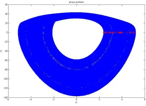
Fig. 2.2 The chaotic attractor of uncontrolled new Double Ge-Ku system………….14

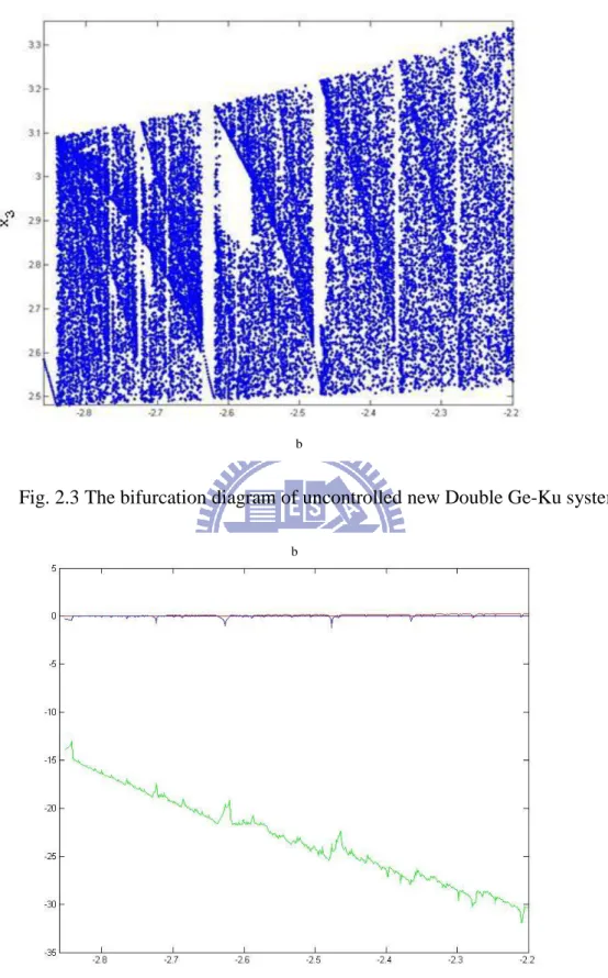
Fig. 2.3 The bifurcation diagram of uncontrolled new Double Ge-Ku system………15

Fig. 2.4.The Lyapunov exponents of uncontrolled new Double Ge-Ku system……..15

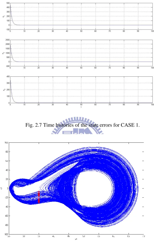
Fig. 2.5 The phase portrait of the controlled new Double Ge-Ku system for CASE 1. ………16

Fig. 2.6 Time histories of the state errors for CASE 1……….16

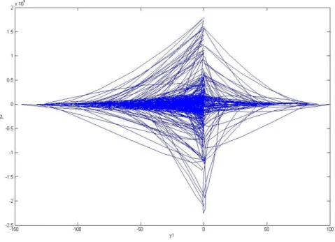
Fig. 2.7 Time histories of x_iy_i and 2 i yi x for CASE 1……….17

Fig. 2.8 The chaotic attractor of a new Ge-Ku-van der Pol system……….17

Fig. 2.9 The phase portrait of the controlled new Double Ge-Ku system for CASE 2 ………18

Fig. 2.10 Time histories of the state errors for CASE 2………18

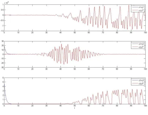
Fig. 2.11 Time histories of x_iy_i and 2 i yi x for CASE 2………...19

Fig. 2.12 The chaotic attractor of a new Ge-Ku Mathieu system………19

Fig. 2.13 The phase portrait of the controlled new Double Ge-Ku system for CASE 3. ………..20

Fig. 2.14 Time histories of the state errors for CASE 3………20

Fig. 2.15 Time histories of x_iy_i and 2 i yi x for CASE 3………21

Fig. 3.1 The chaotic attractor of the Lorenz system……….30

Fig. 3.2 The chaotic attractor of the Chen system………...30

Fig. 3.3 The phase portrait of the controlled DGK system………31

Fig. 3.4 Time histories of the state errors for Case 1………31

(9)

vii

Fig. 3.6 The chaotic attractor of the Rossler system………32

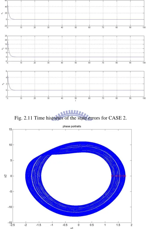
Fig. 3.7 The phase portrait of the controlled DGK system………...33

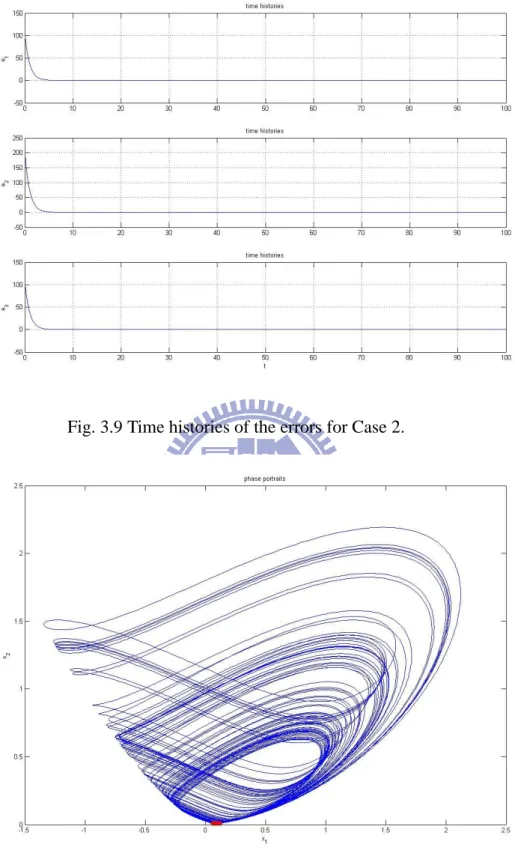
Fig. 3.8 Time histories of the state errors for Case 2………...33

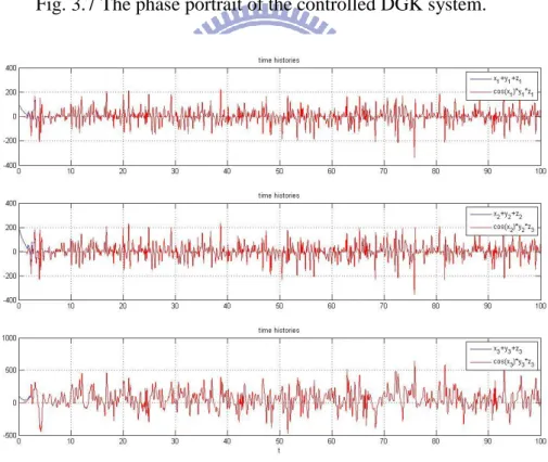
Fig. 3.9 Time histories of G( , , , )x y z t and F x y( , , , )z t for Case 2………..34

Fig. 3.10 The chaotic attractor of a Sprott system………34

Fig. 3.11 The phase portrait of the controlled DGK system………....35

Fig. 3.12 Time histories of the state errors for Case 3………35

Fig. 3.13 Time histories of G( , , , )x y z t and F x y( , , , )z t for Case 3………36

Fig. 4.1 Coordinate translation of state x………49

Fig. 4.2 Coordinate translation of state y……….49

Fig. 4.3 Phase portrait of the error dynamics for Case 1………50

Fig. 4.4 Time histories of errors for Case 1………..50

Fig. 4.5 Time histories of xi, yi for Case 1………..51

Fig. 4.6 Time histories of parameter errors for Case 1……….51

Fig. 4.7 Phase portrait of the error dynamic for Case 2………52

Fig. 4.8 Time histories of errors for Case 2………..52

Fig. 4.9 Time histories of xi, yi for Case 2………53

Fig. 4.10 Time histories of parameter errors for Case 2………53

Fig. 4.11 Phase portrait of the error dynamic for Case 3………54

Fig. 4.12 The chaotic attractor of the Ge-Ku-van der Pol system………....54

Fig. 4.13 Time histories of errors for Case 3………55

Fig. 4.14 Time histories of x_i, y_i for Case 3………55

Fig. 4.15 Time histories of parameter errors for Case 3………...56

Fig. 5.1 The configuration of fuzzy logic controller………70

Fig. 5.2 Membership function………..70

(10)

viii

Fig. 5.4 Projections of phase portrait of Eq (5.19)………...71

Fig. 5.5 Time histories of error derivatives for master and slave chaotic systems without controllers………72

Fig. 5.6 Time histories of states for Example 1 the FLCC is coming into after 30s ………72

Fig. 5.7 Time histories of errors for Example 1 the FLCC is coming into after 30s ………73

Fig. 5.8 Time histories of states for the traditional controller is coming into after 30s ………73

Fig. 5.10 The Rayleigh noise used………...74

Fig. 5.11 Projection of phase portrait of Eq (5.28)………..75

Fig. 5.12 Projections of phase portrait of chaotic DGK systems……….75

Fig. 5.13 Time histories of error derivatives for master and slave chaotic uncertain stochastic systems without controllers……….76

Fig. 5.14 Time histories of states for Example 2 the FLCC is coming into after 30s ………76

Fig. 5.15 Time histories of errors for Example 2 the FLCC is coming into after 30s ………77

Fig. 6.1 Chaotic behavior of Sprott 4 system………...93

(11)

ix

Fig. 6.3 Chaotic behavior of new fuzzy Sprott 4 system with uncertainty…………..94 Fig. 6.4 Chaotic behavior of Rossler system………94 Fig. 6.5 Chaotic behavior of Rossler system with uncertainty……….95 Fig. 6.6 The Rayleigh noise used………95 Fig. 6.7 Chaotic behavior of new fuzzy Rossler system with uncertainty………96 Fig. 6.8 Time histories of errors for Example 1………96 Fig. 6.9 Time histories of errors for Example 2………...97

(12)

1

Chapter 1 Introduction

Chaos is a very interesting nonlinear phenomenon. Chaos as a modern theory is discovered by the age of computer in the middle of the past century, which has an epoch-making significance in exact science.

Generally speaking, designing a system to mimic the behavior of another chaotic system is called synchronization. Synchronization of chaotic systems has received a significant attention, since Pecora and Carroll presented the chaos synchronization method to synchronize two identical chaotic systems with different initial values in 1990 [1].

In recent years , synchronization in chaotic dynamic system is a very interesting problem and has been widely studied. Chaos synchronization has been applied in biological systems [2,3], secure communication [4,5], and many other disciplines. By linear and nonlinear control [6-12] different types of synchronization for interacting chaotic systems, such as complete synchronization [1], phase synchronization [13], lag synchronization [14], generalized synchronization [15-20], anticipating synchronization can be obtained.

Various approaches for achieving chaos synchronization using fuzzy systems have been proposed [21]. Fuzzy set theory was first presented by Zadeh [22], while fuzzy logic control (FLC) schemes have been widely developed and successfully deployed in many applications [23]. Furthermore, adaptive fuzzy controllers have been used to control and synchronize chaotic systems [24,25].

Uncertainties associated with the mathematical characterization of a system can lead to unreliable damage [26]. Probabilistic analysis provides a tool for incorporating randoms in the analysis of frequency response by generally describing the randoms as

(13)

2

randoms variables. While the studies discussed above addressed measurement noise, some researchers have started looking at the effect of noise present in the model. Collins et al. [27] proposed a statistical identification procedure by treating the initial parameters as normally distributed random variables.

In recent years, some chaos synchronizations based on fuzzy systems have been proposed since the fuzzy set theory was initiated by Zadeh [22], such as fuzzy sliding mode controlling technique [28,29], LMI-based synchronization [30] and extended backstepping sliding mode controlling technique [31]. The fuzzy logic control (FLC) scheme have been widely developed and have been successfully applied to many applications [32]. Recently, Yau and Shieh [33] proposed a new idea in designing fuzzy logic controllers - constructing fuzzy rules subject to a common Lyapunov function such that the master-slave chaotic systems satisfy stability condition in the Lyapunov sense. In [33], there are two main controllers in their slave system. One is used in elimination of nonlinear terms and the other is built by fuzzy rules subject to a common Lyapunov function. Therefore, the resulting controllers are in nonlinear form. In [33], the regular form is necessary. In order to carry out the new method, the original system must to be transformed into their regular form.

In recent years, fuzzy logic proposed [34] has received much attention as a powerful tool for the nonlinear control. Among various kinds of fuzzy methods, Takagi-Sugeno fuzzy (T-S fuzzy) system is widely accepted as a useful tool for design and analysis of fuzzy control system [35-40]. Currently, some chaos control and synchronization based on T-S fuzzy systems have been proposed, such as fuzzy sliding mode controlling technique, LMI-based synchronization [41-43] and robust control [44]. Furthermore, two different nonlinear systems may have different numbers of nonlinear terms. It causes different numbers of linear subsystems. For synchronization of two different nonlinear systems, the traditional method using the

(14)

3

idea of PDC to design the fuzzy control law for stabilization of the error dynamics can not be used here, since the number of subsystems becomes very large.

Ge and Ku [45] gave a chaotic system formed by a simple pendulum with its pivot rotating about an axis as Fig. 1.1. This chaotic system is

1 2

2 2 sin [ (1 cos 1) sin ]

x x x ax x b c x d wt          (1.1)

where a b c d are parameters. After simplification, , , , sinx1x1,

2 1 1 cos 1 2 x x   and addition of coupling terms, we get the Double Ge-Ku system









1 2 2 2 2 1 1 3 2 3 3 3 3 1 x x x fx x g h x kx x fx x g h x lx     _{ } _ _ _ _ _  _ _        _   _  (1.2)

where a b c d g, , , , are parameters.

In Chapter 2, a new type of synchronization, double symplectic synchronization, ( , , )t  ( , , )t

G x y F x y is studied. Traditional generalized synchronization and symplectic synchronization are special cases of the double symplectic synchronization. Since the symplectic functions are presented at both the right hand side and the left hand side of the equality. The double symplectic synchronization may be applied to increase the security of secret communication due to the complexity of its synchronization form. By using the Barbalat’s lemma[46], the double symplectic synchronization can be achieved. Finally, the effectiveness and feasibility of our proposed scheme are verified by numerical simulations.

In Chapter 3, a new type of synchronization, multiple symplectic synchronization is studied. When the double symplectic functions are extended to a more general form,

G(x,y,z…w,t) = F(x,y,z…w,t), “multiple symplectic synchronization” is achieved.

(15)

4

secret communication more effectively than double symplectic synchronization due to more complexity of its synchronization form.

In Chapter 4, a new chaos generalized synchronization strategy of different translation pragmatical synchronization by stability theory of partial region [47-49] is proposed. By using the stability theory of partial region, the Lyapunov function is a simple linear homogeneous function of error states, the controllers are more simple since they are in lower degree than that of traditional controllers, while the traditional Lyapunov function is a quadratic form of error states.

In Chapter 5, we propose a new strategy which is also constructing fuzzy rules subject to a Lyapunov direct method. Error derivatives are used to be upper bound and lower bound. Through this new approach, a simplest controller, i.e. constant controller, can be obtained and the difficulty in realization of complicated controllers in chaos synchronization by Lyapunov direct method can be also overcome. Unlike conventional approaches, the resulting control law has less maximum magnitude of the instantaneous control command and it can reduce the actuator saturation phenomenon in real physical system. Some computer simulation examples are given in this Chapter.

In Chapter 6, the new fuzzy model is proposed. It gives a new way to linearize complicated nonlinear system and only two subsystems are concluded. In simulation examples, Sprott 4 system [50] and Rossler system are used.

(16)

5

(17)

6

Chapter 2 Double Symplectic Synchronization

for Double Ge-Ku System

2.1 Preliminary

In this Chapter, a new type of synchronization, double symplectic synchronization,

( , , )t  ( , , )t

G x y F x y is proposed. Double symplectic synchronization is an extension of symplectic synchronization, yF x y( , , )t . Because the symplectic functions are presented at both the right hand side and the left hand side of the equality, it is called “double symplectic synchronization”. Since the synchronization form is more complex than generalized and symplectic synchronizations, so we usually use it on the purpose of secret communication. The scheme is effective as shown by three examples as follows.

2.2 Double Symplectic Synchronization Scheme

Consider two different nonlinear chaotic systems, Partner A and Partner B, described by ( , )t  x f x , (2.1) ( )t ( , )u t   y C y + g u, (2.2) where T 1 2 [ ,x x , ,xn] Rn   x and T 1 2 [ ,y y , ,yn] Rn  

y are the state vectors of Partner A (2.1) and Partner B (2.2), n n

R 



C is the given matrix, f and g are continuous nonlinear vector functions, and u is the controller. Our goal is to design the controller u such that G x y( , , )t asymptotically approaches F x y( , , )t .For simplicity take G x y( , , )t  x y and F x y( , , )t is a continuous nonlinear vector function.

(18)

7

Property 1 [5]: An m n matrix A of real elements defines a linear mapping

yAx from R into n R , and the induced p-norm of m A for p1, 2, and  is given by 1 2 T max 1 2 1 1 max , ( ) , max . m n ij ij j i i j A a A  A A A _ a     



_ _ 



(2.3)

The useful property of induced matrix norms for real matrix A is as follow:

2 1

A  A A_ . (2.4) Theorem: For chaotic systems Partner A (2.1) and Partner B (2.2), if the controller u is designed as 1 ( ) [ ( , ) ( ( ) ( , )) ( , ) ( , ) ( )( ) ( )], t t t t t t t              y x y u I D F D Ff x D F C y g y D F f x g y C x F K x y F (2.5)

where D Fx , D Fy , D Ft are the Jacobian matrices of F x y( , , )t ,

1 2 diag( ,k k , ,km)  K , and satisfies min( ) 1 ( ) i k t  C , (2.6)

then the double symplectic synchronization will be achieved.

Proof: Define the error vectors as

( , , )t

  

e x y F x y , (2.7)

then the following error dynamics can be obtained by introducing the designed controller ( , ) ( ) ( , ) ( , ) ( ( ) ( , )) ( ) ( ( ) ) . t t d dt t t t t t t t                  x y x y y e e x y D Fx D Fy D F f x C y g y D Ff x D F C y g y D F I D F u C K e (2.8)

(19)

8 T 1 ( ) 2 V t  e e. (2.9)

Taking the time derivative of V t( ) along the trajectory of Eq. (2.8), we have T T T 2 2 2 ( ) ( ) ( ) min( ) ( ( ) min( )) . i i V t t t k t k         e e e C e e Ke C e e C e (2.10)

Since M min( )k_i  C( )t 0, then V t( ) M e 2  2MV t( ). Therefore, it can be obtained that

2 ( ) (0)e Mt V t V  (2.11) and 0 lim t ( )

t



V  d is bounded. Besides, V t( ) is uniformly continuous. According

to Barbalat’s lemma [46], the conclusion can be drawn that lim ( ) 0

tV t  , i.e.

lim ( ) 0

t e t  . Thus, the double symplectic synchronization can be achieved

asymptotically.

2.3 Synchronization of Two Different New Chaotic Systems

CASE 1

Consider a new Ge-Ku-Duffing(GKD) system as Partner A described by

(2.12)

where h=0.1; l=11; p=40; k=54; f=6; g=30; and the initial conditions are 1(0) 2, (0)2 2.4 , (0)3 5

x  x  x  . Eq. (2.12) can be rewritten in the form of Eq. (2.1),





1 2 2 2 2 1 1 3 3 3 3 3 2 1 x x x hx x l p x kx x x x fx gx    _{ } _ _ _ _ _  _ _       

(20)

9 where





2 2 2 1 1 3 3 3 3 2 1 ( , ) x t hx x l p x kx x x fx gx          _   _           f x

. The chaotic attractor of the new

GKD system is shown in Fig. 2.1.

The controlled new Double Ge-Ku (DGK) system is considered as Partner B described by

(2.13)

where a=-0.5; b=-1.4; c=1.9; d=-4.5; e=6.2;, u



u u u1, 2, 3



T is the controller, and the initial condition is y1(0)2, y2(0)2.4, y3(0)5.

The chaotic attractor of uncontrolled new DGK system is shown in Fig. 2.2, Bifurcation diagram in Fig. 2.3 and Lyapunov exponents in Fig. 2.4. Eq. (2.13) can be

rewritten in the form of Eq. (2.2), where

0 1 0 ( ) 0 0 0 t bc a a bc      _  _       C and 3 1 1 3 3 3 1 3 0 ( , )t by dy y by ey y     _  _     

g y . By applying Property 1, it is derived that C( )t ₁   a bc

( )t _   a bc C , and C( )t ₂  ( a bc)2  9.9856 . Then C( )t 3.1 is estimated. Define 2 1 1 2 2 2 2 3 3 ( , , ) x y t x y x y           

F x y , and our goal is to achieve the double symplectic

synchronization x y F x y( , , )t . According to Theorem, the inequality min( ) 1 ( )

i

k

t 

C

must be satisfied. It can be obtained that min( )ki 3.1 if we choose









1 2 1 2 2 2 1 1 3 2 2 3 3 3 3 1 3 y y u y ay y b c y dy u y ay y b c y ey u      _{ } _ _ _ _ __  _ _        _   _ 

(21)

10 1 2 3 0 0 4 0 0 0 0 0 5 0 0 0 0 0 6 k k k         _ _{ } _        

K and design the controller as

2 2 1 2 1 1 2 1 2 2 2 1 1 1 1 u  x y x x y  x y x y  x y 2 2 2 2 2 2 2 2 1 1 3 2 2 1 1 3 2 1 1 3 2 2 2 1 1 3 2 2 2 2 2 { [ ( ) ]} { [ ( ) ]} [ ( ) ] [ ( ) ] u x y hx x l p x kx x ay y b c y dy hx x l p x kx ay y b c y dy x y x y                      3 2 2 3 3 3 3 3 3 2 1 3 3 3 3 1 3 3 2 1 2 2 3 3 3 1 3 3 3 3 2 ( ) { [ ( ) ]} [ ( ) ] u x y x x fx gx x ay y b c y ey x x fx gx ay y b c y ey x y x y                     

The Theorem is satisfied and the double symplectic synchronization is achieved. The phase portrait of the controlled DGK system and the time histories of the state errors are shown in Fig. 2.5 and Fig. 2.6 and Fig. 2.7, respectively.

CASE 2

Consider a new Ge-Ku-van der Pol(GKv) system as Partner A described by

(2.14)

where f=0.08; p=-0.35; k=100.56; m=-1000.02; g=0.61; h=0.08; l=0.01; and the initial conditions are (0)x1 0.01, (0)x2 0.01 , (0)x3 0.01. Eq. (2.14) can be

rewritten in the form of Eq. (2.1) , where

2 2 2 3 1 3 2 3 3 2 1 ( , ) [ ( ) (1 ) x t fx x p k x mx gx h x x lx      _    _ _ _ _ _    f x .

The chaotic attractor of the GKv system is shown in Fig.2.8.

The controlled DGK system is considered as Partner B described by

(2.15)









1 2 2 2 2 3 1 3 2 3 3 1 3 2 1 x x x fx x p k x mx x gx h x x lx    _{ } _ _ _ _ _  _ _       









1 2 1 2 2 2 1 1 3 2 2 y y u y ay y b c y dy u      _{ } _ _ _ _ __  _ _          

(22)

11

where a=-0.5; b=-1.4; c=1.9; d=-4.5; e=6.2; , u



u u u1, 2, 3



T is the vector controller, and the initial conditions are y₁(0)0.01, y₂(0)0.01, y₃(0)0.01.

Eq. (2.15) can be rewritten in the form of Eq. (2.2), where

0 1 0 ( ) 0 0 t bc a l g      _  _      C and 13 1 3 3 3 1 3 0 ( , )t by dy y by ey y     _  _     

g y . By applying Property 1, it is derived that

1 ( )t   a bc, C C( )t _   a bc , and 2 2 ( )t  ( a bc)  9.9856 C . Then ( )t 3.1 C is estimated. Define 2 1 1 2 2 2 2 3 3 ( , , ) x y t x y x y           

F x y , and our goal is to achieve the double symplectic

synchronization x y F x y( , , )t . According to Theorem, the inequality min( ) 1 ( ) i k t 

C must be satisfied. It can be obtained that min( )ki 3.1. Thua we

choose 1 2 3 0 0 4 0 0 0 0 0 5 0 0 0 0 0 6 k k k         _ _{ } _        

2 2 1 2 1 1 2 1 2 2 2 1 1 1 1 u  x y x x y  x y x y  x y 2 2 2 2 2 2 2 2 3 1 3 2 2 1 1 3 2 3 1 3 2 2 2 1 1 3 2 2 2 2 2 { [ ( ) ]} { [ ( ) ]} [ ( ) ] [ ( ) ] u x y fx x p k x mx x ay y b c y dy fx x p k x mx ay y b c y dy x y x y                      2 2 2 2 3 3 3 3 3 2 1 3 3 3 3 1 3 3 2 1 2 2 3 3 3 1 3 3 3 3 2 [ (1 ) ] { [ ( ) ]} (1 ) [ ( ) ] u x y gx h x x lx x ay y b c y ey gx h x x lx ay y b c y ey x y x y                     

(23)

12

The phase portrait of the controlled DGK system and the time histories of the errors are shown in Fig.2.9, Fig.2.10 and Fig.2.11, respectively.

CASE 3

Consider the Ge-Ku Mathieu(GKM) system as Partner A described by

(2.16)

where k=-0.6; f=5; m=11; n=0.3; g=8; h=10; l=0.5; p=0.2; and the initial conditions are x₁(0)0.01, (0)x₂ 0.01 , (0)x₃ 0.01 Eq. (2.16) can be rewritten in

the form of Eq. (2.1), where





2 2 2 1 1 2 3 1 3 2 1 3 ( , ) ( ) x t kx x f m x nx x g hx x lx px x    _ _  _  _   __           f x .The chaotic

attractor of the GKM system is shown in Fig.2.12.

The controlled DGK system is considered as Partner B described by

(2.17)

where a=-0.5; b=-1.4; c=1.9; d=-4.5; e=6.2; , u



u u u1, 2, 3



T is the vector controller, and the initial conditions are y₁(0)0.01, y₂(0)0.01, y₃(0)0.01.

Eq. (2.17) can be rewritten in the form of Eq. (2.2), where

0 1 0 ( ) 0 0 t bc a l g      _  _      C and 13 1 3 3 3 1 3 0 ( , )t by dy y by ey y     _  _     

g y . By applying Property 1, it is derived that













1 2 2 2 2 1 1 2 3 3 ( 1) 3 2 1 3 x x x kx x f m x nx x x g hx x lx px x            _ _       

(24)

13 1 ( )t   a bc, C C( )t _   a bc , and 2 2 ( )t  ( a bc)  9.9856 C . Then ( )t 3.1 C is estimated. Define 2 1 1 2 2 2 2 3 3 ( , , ) x y t x y x y           

F x y , and our goal is to achieve the

double symplectic synchronization x y F x y( , , )t . According to Theorem, the inequality min( ) 1

( )

i

k

t 

C must be satisfied. It can be obtained that min( )ki 3.1.

Thus we choose 1 2 3 0 0 4 0 0 0 0 0 5 0 0 0 0 0 6 k k k         _ _{ } _        

2 2 1 2 1 1 2 1 2 2 2 1 1 1 1 u  x y x x y  x y x y  x y 2 2 2 2 2 2 2 2 1 1 2 3 2 2 1 1 3 2 1 1 2 3 2 2 2 1 1 3 2 2 2 2 2 { [ ( ) ]} { [ ( ) ]} [ ( ) ] [ ( ) ] u x y kx x f m x nx x x ay y b c y dy kx x f m x nx x ay y b c y dy x y x y                      2 2 3 3 3 1 3 2 1 3 3 3 3 3 1 1 3 2 1 3 2 2 3 3 3 1 3 3 3 3 2 [ ( ) ] { [ ( ) ]} ( ) [ ( ) ] u x y g hx x lx px x x ay y b c y ey g hx x lx px x ay y b c y ey x y x y                     

The Theorem is satisfied and the double symplectic synchronization is achieved. The phase portrait of the controlled DGK system and the time histories of the state errors are shown in Fig2.13, Fig.2.14 and Fig.2.15, respectively.

(25)

14

Fig. 2.1 The chaotic attractor of a new Ge-Ku-Duffing system.

(26)

15

Fig. 2.3 The bifurcation diagram of uncontrolled new Double Ge-Ku system.

Fig. 2.4.The Lyapunov exponents of uncontrolled new Double Ge-Ku system. b

(27)

16

Fig. 2.5 The phase portrait of the controlled new Double Ge-Ku system for CASE 1.

Fig. 2.6 Time histories of x_iy_i and 2

i yi

(28)

17

Fig. 2.7 Time histories of the state errors for CASE 1.

(29)

18

i yi

(30)

19

Fig. 2.11 Time histories of the state errors for CASE 2.

(31)

20

i yi

(32)

21

(33)

22

Chapter 3 Multiple Symplectic Synchronization

for Double Ge-Ku

System

3.1 Preliminary

In this Chapter, a new type of synchronization, multiple symplectic synchronization is studied. Symplectic synchronization and double symplectic synchronization are special cases of the multiple symplectic synchronization. When

the double symplectic functions is extended to a more general form,

G(x,y,z…w,t) = F(x,y,z…w,t) , it is called “multiple symplectic synchronization”.

The multiple symplectic synchronization may be applied to increase the security of secret communication due to the complexity of its synchronization form.

3.2 Multiple Symplectic Synchronization Scheme

Chaos synchronization, first proposed by Fujisaka and Yamada in 1983, did not received great attention until 1990. Among many kinds of synchronizations, the generalized synchronization is investigated. It means there exist a functional relationship between the states of the master and those of the slave. Symplectic synchronization is defined as yH x y t( , , ), where x, y are the state vectors of the “master” and of the “slave”, respectively. The final desired state y of the “slave” not only depends upon the “master” state x but also depends upon the “slave” state y itself. Therefore the “slave” is not a traditional pure slave obeying the “master” completely but plays a role to determine the final desired state of the “slave” system. We call this kind of synchronization, “symplectic synchronization”, and call the “master” system Partner A, the “slave” system Partner B.

(34)

23

left hand side of the equality, it is called double symplectic synchronization, ( , , )t  ( , , )t

G x y F x y , where x, y are state vectors of Partner A and Partner B, respectively, G x y( , , )t and F x y( , , )t are given vector functions of x, y and time.

When the double symplectic functions is extended to a more general form,

G(x,y,z… w,t) = F(x,y,z… w,t), is called “multiple symplectic synchronization”,

where x y, , ,z ,ware state vectors of Partner A and Partner B, respectively,

G(x,y,z…w,t)and F(x,y,z…w,t)are given vector functions of x y, , ,z ,w_{and time.}

3.3 Synchronization of Three Different Chaotic Systems

CASE 1.

Define 1 1 1 2 2 2 3 3 3 ( , , , ) x y z z t x y z x y z       _   _       G x y ,





































1 1 1 2 2 1 3 3 1 1 1 2 2 2 2 3 3 2 1 1 3 2 2 3 3 3 3

sin sin sin ( , , , ) sin sin sin sin sin sin

x y z x y z x y z z t x y z x y z x y z x y z x y z x y z       _   _       F x y ,

and we wish to achieve the multiple symplectic synchronization

G(x,y,z,t) = F(x,y,z,t).

Let e = G(x,y,z,t) - F(x,y,z,t)

Consider a Lorenz system is described by

(3.1)

where w₁ 10, w₂ 8, w₃ 28, 3

   and the initial condition is

1 2 3

(0)x 0.01, (0)x 0.01 , (0)x 0.01. The chaotic attractor of the Lorenz system is shown in Fig. 3.1.

The Chen system is described by

1 1 1 1 2 2 3 1 2 1 3 3 2 3 1 2 x w x w x x w x x x x x w x x x              





1 1 2 1 2 2 1 1 1 3 2 2 3 1 2 3 3 ( ) z h z z z h h z z z h z z z z h z             

(35)

24

(3.2)

where h135,h2 27.2,h33, and the initial condition is

1 2 3

z (0)0.5, z (0)0.26 ,z (0)0.35. The chaotic attractor of the Chen system is shown in Fig. 3.2.

The controlled Double Ge-Ku (DGK) system is described by

(3.3)

where a=-0.5; b=-1.4; c=1.9; d=-4.5; e=6.2, is the controller parameters, and the initial condition is y (0)1 0.01, y (0)2 0.01 ,y (0)3 0.01,.

Thus we design the controller as







 











 



















 





















1 1 1 1 2 2 1 2 1 1 1 1 2 1 1 1 2 1 1 1 1 1 2 1 3 1 2 1 3 2 1 2 2 2 1 1 3 2 1 2 2 1 2 1 2 2 3 1 2 3 1 3 3 3 3 1 3 1 3 sin

cos sin sin

cos sin sin cos u w x w x y h z z w x w x y z x y y z x y h z z w x x x x y z x ay y b c y dy y z x y h z z w x x x y z x ay y b c y ey y z x      _  _     _  _        _   _  _  _         _   _ 



sin y₃

 

_h z₁ ₂z₁



_





























 























 



2 2 3 1 2 1 3 2 1 1 3 2 1 1 1 3 2 2 1 1 1 2 1 2 1 2 1 2 1 1 2 1 1 1 3 2 2 3 1 2 1 3 2 2 2 2 2 1 1 3 2 2 2 2 2 1 1 1 3 2 2 sin cos sin sin cos sin u w x x x x ay y b c y dy h h z z z h z w x w x y z x y y z x y h h z z z h z w x x x x y z x ay y b c y dy y z x y h h z z z h z          _   _ _    _     _    _        _   _  _    _ 





















 



2 2 3 1 2 3 2 3 3 3 3 1 3 2 3 3 2 1 1 1 3 2 2 sin cos sin w x x x y z x ay y b c y ey y z x y h h z z z h z        _   _  _    _









(36)

25















 













 

































2 3 2 3 1 2 3 3 3 1 1 2 3 3 1 1 1 2 1 3 1 2 1 3 1 1 1 2 3 3 3 1 2 1 3 2 3 2 2 2 1 1 3 2 3 2 2 1 2 3 3 2 2 3 1 2 3 3 3 3 3 3 1 sin cos sin sin cos sin sin u w x x x ay y b c y ey z z h z w x w x y z x y y z x y z z h z w x x x x y z x ay y b c y dy y z x y z z h z w x x x y z x ay y b c y ey          _   _                 _   _       



   













3 3 3 3 1 2 3 3 cos sin y z x y z z h z     

The Theorem in Chapter 2 is satisfied and the multiple symplectic synchronization is achieved. The phase portrait of the controlled DGK system and the time histories of the state errors and the time histories of G( , , , )x y z t and F x y( , , , )z t are shown in Fig. 3.3 and Fig. 3.4 and Fig. 3.5, respectively.

CASE 2.

Define 1 1 1 2 2 2 3 3 3 ( , , , ) x y z z t x y z x y z       _   _       G x y , ,

and we wish to achieve the multiple symplectic synchronization

G(x,y,z,t) = F(x,y,z,t).

Consider a Rossler system is described by

(3.4)

where w10.15, w2 0.2, w3 10, and the initial condition is

1 2 3

(0)x 2, (0)x 2.4, (0)x 5,. The chaotic attractor of the Rossler system is shown in Fig. 3.6.





































1 1 1 2 2 1 3 3 1 1 1 2 2 2 2 3 3 2 1 1 3 2 2 3 3 3 3

cos cos cos

( , , , ) cos cos cos

cos cos cos

x y z x y z x y z z t x y z x y z x y z x y z x y z x y z       _   _       F x y 1 2 3 2 1 1 2 3 2 1 3 3 3

x

w x

x

w

x x

w x

  



  



  





(37)

26 The Chen system is described

(3.5)

where h135,h2 27.2,h33, and the initial condition is

1 2 3

z (0)0.5, z (0)0.26 ,z (0)0.35.

The controlled DGK system is described by

(3.6)

where a=-0.5; b=-1.4; c=1.9; d=-4.5; e=6.2, is the controller parameters, and the initial condition is y (0)₁ 0.01, y (0)₂ 0.01 ,y (0)₃ 0.01,.







 















 















































1 2 3 2 1 2 1 2 3 1 1 1 1 2 1 1 1 1 2 1 1 1 2 2 2 1 2 2 2 1 1 3 1 2 2 1 2 1 2 2 1 3 3 3 3 3 1 3 3 3 3 1 1 3 3 1 2 sin

cos cos sin

cos cos sin cos cos u x x y h z z x x x y z x y z x y h z z x w x x y z x ay y b c y dy z x y h z z w x x w x x y z x ay y b c y ey z x y h z z      _  _     _  _       _   _  _  _         _   _  _



 ₁



_





























 























 







2 2 1 1 2 2 1 1 3 2 1 1 1 3 2 2 2 3 1 1 2 1 2 2 1 1 2 1 1 1 3 2 2 2 1 1 2 2 2 2 2 2 1 1 3 2 2 2 2 1 1 1 3 2 2 2 1 3 3 3

sin cos cos

sin cos cos si u x w x ay y b c y dy h h z z z h z x x x y z x y z x y h h z z z h z x w x x y z x ay y b c y dy z x y h h z z z h z w x x w x         _   _ _    _      _    _        _   _  _    _  



















 



3 3 2 2 3 3 3 3 1 2 3 3 2 1 1 1 3 2 2 n cos cos x y z x ay y b c y ey  z x y h h z z z h z    _   _  _    _





1 1 2 1 2 2 1 1 1 3 2 2 3 1 2 3 3 ( ) z h z z z h h z z z h z z z z h z             









(38)

27





























 























 













2 3 2 1 3 3 3 3 3 3 3 1 2 3 3 2 3 1 1 3 1 2 3 1 1 1 2 3 3 2 1 1 2 2 2 3 2 2 1 1 3 3 2 2 1 2 3 3 2 1 3 3 3 3 3 3 2 3 3 3 3 1

sin cos cos

sin cos cos sin cos u w x x w x ay y b c y ey z z h z x x x y z x y z x y z z h z x w x x y z x ay y b c y dy z x y z z h z w x x w x x y z x ay y b c y ey          _   _                _   _       



  _   _



z₃



cosx₃

 

y z z₃ _{1 2}h z_{3 3}



The Theorem in Chapter 2 is satisfied and the multiple symplectic synchronization is achieved. The phase portrait of the controlled DGK system and the time histories of the state errors and the time histories of G( , , , )x y z t and F x y( , , , )z t are shown in Fig. 3.7 and Fig. 3.8 and Fig. 3.9, respectively.

CASE 3.

Define 1 1 1 2 2 2 3 3 3 ( , , , ) x y z z t x y z x y z       _   _       G x y , ,

and we wish to achieve the multiple symplectic synchronization.

G(x,y,z,t) = F(x,y,z,t).

Consider a Sprott E system is described by

(3.7)

where w14, and the initial condition is (0)x1  1, (0)x2  1, (0)x3  1,. The chaotic attractor of the Sprott E system is shown in Fig. 3.10.

The Chen system is described

1 1 1 2 2 1 3 3 1 1 1 2 2 2 2 3 3 2 1 1 3 2 2 3 3 3 3 ( , , , ) x y z x y z x y z z t x y z x y z x y z x y z x y z x y z       _   _       F x y 1 2 3 2 2 1 2 3 1 1 1 x x x x x x x w x    _ _     

(39)

28

(3.8)

where h135, h2 27.2, h3 3, and the initial condition is

1 2 3

z (0)0.5, z (0)0.26, z (0)0.35.

The controlled DGK system is described by

(3.9)

where a=-0.5; b=-1.4; c=1.9; d=-4.5; e=6.2, are the controller parameters, and the initial condition is y (0)1 0.01, y (0)2 0.01 ,y (0)3 0.01,.























 















1 2 3 2 1 2 1 2 3 1 1 1 2 1 1 1 1 2 1 2 2 1 2 2 1 2 2 1 1 3 1 2 2 2 1 2 1 1 1 3 1 3 3 3 3 1 1 3 3 1 2 1 1 u x x y h z z x x y z x y z x y h z z x x y z x ay y b c y dy z x y h z z w x y z x ay y b c y ey z x y h z z    _  _   _  _        _   _    _  _     _   _  _  _

















































2 2 2 1 2 2 1 1 3 2 1 1 1 3 2 2 2 2 3 1 2 1 2 2 1 1 2 1 1 1 3 2 2 1 2 2 2 2 2 2 1 1 3 2 2 2 2 1 1 1 3 2 2 2 1 1 3 2 3 3 3 3 1 2 3 1 u x x ay y b c y dy h h z z z h z x x y z x y z x y h h z z z h z x x y z x ay y b c y dy z x y h h z z z h z w x y z x ay y b c y ey z x y         _   _ _    _    _    _       _   _  _    _        _   _  ₃_



h₂h z₁



₁z z_{1 3}h z_{2 2}_





















































2 3 1 1 3 3 3 1 1 2 3 3 2 2 3 1 3 1 2 3 1 1 1 2 3 3 1 2 2 3 2 2 2 1 1 3 3 2 2 1 2 3 3 2 1 1 3 3 3 3 3 3 1 3 3 3 1 2 3 3 1 1 u w x ay y b c y ey z z h z x x y z x y z x y z z h z x x y z x ay y b c y dy z x y z z h z w x y z x ay y b c y ey z x y z z h z         _   _              _   _          _   _  

The Theorem in Chapter 2 is satisfied and the multiple symplectic synchronization





1 1 2 1 2 2 1 1 1 3 2 2 3 1 2 3 3

(

)

z

h z

z

h

h z

z z

h z

z

z z

h z







  







 













(40)

29

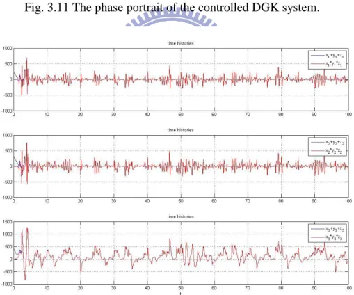
is achieved. The phase portrait of the controlled DGK system and the time histories of the state errors and the time histories of G( , , , )x y z t and F x y( , , , )z t are shown in Fig. 3.11 and Fig. 3.12 and Fig. 3.13, respectively.

(41)

30

Fig. 3.1 The chaotic attractor of the Lorenz system.

(42)

31

Fig. 3.3 The phase portrait of the controlled DGK system.

(43)

32

Fig. 3.5 Time histories of the errors for Case 1.

(44)

33

(45)

34

Fig. 3.9 Time histories of the errors for Case 2.

(46)

35

(47)

36

(48)

37

Chapter 4 Different Translation Pragmatical Generalized

Synchronization by Stability Theory of Partial Region for

Double Ge-Ku System

4.1 Preliminary

In this Chapter, a new strategy to achieve different translation generalized synchronization by stability theory of partial region by which the Lyapunov function is simple linear homogeneous function of error states, the controllers are more simple since they are in lower degree than that of traditional controllers.

By a pragmatical theorem of asymptotical stability based on an assumption of equal probability of initial point, an adaptive control law is derived such that it can be proved strictly that the common zero solution of error dynamics and of parameter dynamics is asymptotically stable. Numerical simulations of a new Double Ge-Ku(DGK) system are given to show the effectiveness of the proposed scheme.

4.2 The Scheme of Different Translation Pragmatical Generalized

Synchronization by Stability Theory of Partial Region

There are two identical nonlinear dynamical systems, and the master system synchronizes the slave system. The master system is given by

x A x ( ,f x B) (4.1) The master system after the origin of x-coordinate system is translated to 1 1 1

( , ,k k , )k _is

x A x (f x B, ) ( 4 . 1 ) where x[ ,x x₁ ₂,,xn]T   x k₁ [x₁k x₁, ₂k₁, ,xnk₁]Rn denotes a state

(49)

38

vector where k1[ , ,k k1 1 , ]k1 _{is a constant vector with positive coefficient} k1_as shown in Fig.4.1. A is an n n uncertain constant coefficients matrix, f is a nonlinear vector function, and B is a vector of uncertain constant coefficients in f .

The slave system is given by

y A y ( ,f y B) ( )u t (4.2) The slave system after the origin of y-coordinate system is translated to

2 2 2

( ,k k , ,k )_is

y A y (f ,y B) ( )u t ( 4 . 2 ) where y[ ,y y₁ ₂,,y_n]T  y k₂ [y₁k y₂, ₂k₂, ,y_nk₂]Rn denotes a state vector where k2 is a constant vector with positive coefficient k2 as shown in

Fig.4.2. A is an n n estimated coefficient matrix, B is a vector of estimated coefficients in f , and u t( )[ ( ),u t u t₁ ₂( ),,u tn( )]TRn is a control input vector.

Our goal is to design a controller u t( ) so that the state vector of the translated slave system (4.2) asymptotically approaches the state vector of the translated master system (4.1) plus a given nonchaotic or chaotic vector function

1 2

( ) [ ( ), ( ), , _n( )]T

F t  F t F t  F t ：

y G x( ) x F t( ). (4.3) This generalized synchronization can be accomplished when t, the limit of the error vector e t( )[ ,e e₁ ₂,,e_n]Tapproaches zero:

l i mte (4.4) 0

where

e x  F t( )  y x y( )F t. (4.5) From Eq. (4.5) we have

(50)

39

e  x y F t( ) (4.6) e A x  A y  ( f x B, )  ( f,y B) ( )F t . (4.7) ( )u t where k₁ and k₂ are chosen to guarantee that the error dynamics always occurs in the first quadrant of e coordinate system.

A Lyapunov function V e A B( , c, c)is chosen as a positive definite function in first

quadrant of e coordinate system by stability theory in partial region as shown in Appendix A：

V e A( , c , Bc  ) e cA (4.8) cB

where Ac A A , Bc  B B , A and c B are two column matrices whose c

elements are all the elements of matrix A and of matrix c B , respectively. c

Its derivative along any solution of the differential equation system consisting of Eq. (4.7) and update parameter differential equations for A and c B is c

V e A B( , c ,c ) AxAy f x B( , f y B)  ( ,F t) u t( )Ac( )Bc (4.9)

where u t( ), A , and c Bc are chosen so that V Ce, C is a diagonal negative

definite matrix, and V is a negative semi-definite function of e and parameter differences A and c Bc. By pragmatical asymptotically stability theorem in Appendix

B, the Lyapunov function used is a simple linear homogeneous function of states and the controllers are simpler because they in lower order than that of traditional controllers. In many papers [51-55], traditional Lyapunov stability theorem and Babalat lemma are used to prove the error vector approaches zero, as time approaches infinity. But the question, why the estimated parameters also approach to the uncertain parameters, remains no answer. By pragmatical asymptotical stability theorem, the question can be answered strictly.

雙 Ge-Ku系統,Sprott 4系統及 Rossler系統的渾沌與渾沌同步

國 立 交 通 大 學

機械工程學系

碩士論文