一個無線區域網路上支援即時影音傳輸的適應性輪詢機制

全文

(1)國立交通大學網路工程研究所碩士論文. 一個無線區域網路上支援即時影音傳輸的適應性輪詢機制 An Adaptive Polling Scheme Supporting Real-Time Audio/Video Transmission in Wireless LANs. 研究生：葉函儒指導教授：陳耀宗教授. 中華民國九十六年七月.

(2) 一個無線區域網路上支援即時影音傳輸的適應性輪詢機制 An Adaptive Polling Scheme Supporting Real-Time Audio/Video Transmission in Wireless LANs. 研究生：葉函儒. Student：Han-Ru Yeh. 指導教授：陳耀宗. Advisor：Yaw-Chung Chen. 國立交通大學網路工程研究所碩士論文. A Thesis Submitted to Institute of Network Engineering College of Computer Science National Chiao Tung University in partial Fulfillment of the Requirements for the Degree of Master in Computer Science June 2007 Hsinchu, Taiwan, Republic of China. 中華民國九十六年七月.

(3) 一個無線區域網路上支援即時影音傳輸的適應性輪詢機制研究生：葉函儒. 指導教授：陳耀宗. 國立交通大學網路工程所. 摘要 IEEE 802.11e 標準主要是為了提供無線區域網路上的服務品質(QoS)。然而它卻依然無法做到即時媒體傳輸的品質保證，同時也會產生不少頻寬的浪費。本篇論文提出一種新的輪詢機制以達到更好的服務品質，像是改進時間顫動(jitter)、減少存取延遲(access delay)，以及提高頻寬的使用率。我們提出一個適應性的輪詢機制，此機制基於不同的工作站需要不同的服務區間，計算出每個工作站更合適的輪詢時間，以避免被輪詢到的工作站沒有訊框可以傳送，而造成浪費。不同的影音編碼方式，也會在這個新的輪詢機制考量範圍內。此外，為了偵測出更合適的輪詢時間以減少存取延遲，我們會在短暫的時間內，使用較短的服務區間來輪詢。同時我們會動態地增減語音傳輸資料流的服務區間，來適應此語音類型資料流的特徵。我們利用 NS-2 進行模擬實驗，數據結果顯示，我們提出的方法比起慣用的輪詢機制，可以減少更多存取延遲，也能降低時間顫動的標準差，同時提高整個無線頻寬的使用率。. i.

(4) An Adaptive Polling Scheme Supporting Real-Time Audio/Video Transmission in Wireless LANs Student: Han-Ru Yeh. Advisor: Yaw-Chung Chen Institute of Network Engineering National Chiao Tung University. Abstract The main goal of IEEE 802.11e standard is to support Quality of Service (QoS) in wireless local area networks (WLANs). However, it makes a lot of unnecessary overheads and is still unable to guarantee QoS for real-time audio/video services. The motivation of this thesis is to provide better QoS, such as reducing jitter and access delay, and to improve the channel utilization. We propose an adaptive polling scheme which minimizes QoS-Null replies by calculating much appropriate polling time for all QoS traffic streams, based on much accurate service intervals for different QoS traffic streams. Also different codecs are taken into consideration in our proposed scheme. Besides, in order to reduce access delay and find a much precise polling time, we reduce polling interval to poll some traffic streams. Further, we dynamically increase or decrease service interval for voice transmission based on its talk-spurt and silence alternation characteristic. The simulation results through NS-2 show that our proposed scheme can reduce access delay and standard deviation of jitter as well as enhance channel throughput comparing with the commonly used round-robin polling scheme.. Keywords: QoS, jitter, access delay, polling scheme ii.

(5) Acknowledgement. First of all, I would like to express my sincerity to the Prof. Yaw-Chung Chen who gave me a lot of precious suggestions, supported me with his experience, professional knowledge and valuable time. He guided me through the difficulties to a proper goal and inspired me so much to complete this thesis. I would also appreciate my family for their encouragement and trust all the time. Besides, I need to thank my laboratory mates Chun-Yung Lin, Cheng-Yuan Ho, Zhen-Hua Shi, and my roommate Cheng-Han Jiang. They gave me many useful comments. Finally, I would like to thank all members in my laboratory for the wonderful time.. iii.

(6) Table of Contents 摘要. ………………………………………………………………………………….i. Abstract …………………………………………………………………………………ii Acknowledgement ……………………………………………………………………...iii List of Figures ………………………………………………………………………vi List of Tables ..........................................................................................................vii List of Equations ..........................................................................................................vii Chapter 1 Introduction …………………………………………………………….1 Chapter 2 Background and Related Work ……………………………………….6 2.1 Review of IEEE 802.11 MAC …………………………………………….6 2.1.1 Distributed Coordination Function …………………………….6 2.1.2 Point Coordination Function ………………………………….8 2.2 Introduction to IEEE 802.11e ………………………………………….10 2.2.1 Enhanced Distributed Channel Access (EDCA) …………...11 2.2.2 HCF Controlled Channel Access (HCCA) ……………………...14 2.3 Summary of WLAN MAC Mechanisms …………………………...17 2.4 Attributes of Real-Time Multimedia ………………………………...18 2.5 Related Works ……………………………………………………….......20 Chapter 3 Proposed Polling Scheme ………………...........................................22 3.1 Main Architecture ……………………………………………………...23 3.2 Polling Scheduling Mechanism ……………………………………...24 3.2.1 Time-Stamp Poll Scheduling ………………………………...24 3.2.2 Polling Policy and Priority ……………………………………...28 3.2.3 Jitter Deviation Reduction ……………………………………...29 3.3 Access Delay Reduction ………………………………………………...32 3.3.1 Relationship of Frame Arriving Time and Access Delay ……...32 3.3.2 Short Interval Polling Function ………………………………...33 3.4 Talk-spurt and Silence Detection and Management ………………...35 3.5 Polling List Table ……………………………………………………...38 3.5.1 Polling List Format …………………………………………...38 3.5.2 Polling List Update …………………………………………...40 3.6 TXOP Calculation ……………………………………………………...41 3.7 Admission Control ……………………………………………………...43 3.8 Summary ………………………………………………………………...45 Chapter 4 Simulation and Numerical Results ………………………………...47 4.1 Simulation environment ………………………………………………...47 4.2 Numerical Result Analysis …………………………………………...48 4.2.1 Throughput Enhancement …………………………………………...49 iv.

(7) 4.2.2 Jitter Deviation Reduction …………………………………………...51 4.2.3 Access Delay Improvement …………………………………………...52 Chapter 5 Conclusion and Future Works ………………………………….…..54 References …………………………………………………………………………...56. v.

(8) Table of Figures Figure 2.1 DCF transmission scheme …………………………………………………………….7 Figure 2.2 DSSS contention window size ………………………………………………………7 Figure 2.3 DCF timing chart. ………………………………………………………………….8. Figure 2.4 PCF timing chart. ………………………………………………………………….9. Figure 2.5 MAC architecture. ………………………………………………………………10. Figure 2.6 MAC frame format ………………………………………………………………...11 Figure 2.7 reference implementation model. .………………………………………………12. Figure 2.8 IFS relationship and related terms. ……………………………………………….14. Figure 2.9 TSPEC element format. …………………………………………………………..15. Figure 2.10 CAP/CFP/CP/SI periods …………………………………………………………...16 Figure 3.1 AP decision flow chart. ………………………………………………………...…24. Figure 3.2 Illustration of traditional RR polling scheme. ……………………………………26. Figure 3.3 Illustration of adaptive time-stamp polling scheme th. Figure 3.4 Illustration of n polling with responding data. ……………………………...27. ……………………………………30. th. Figure 3.5 Illustration of polling with responding m data ……………………………………30 Figure 3.6 Relationship of frame arriving time and access delay …………………………...…33 Figure 3.7 Illustration of short interval polling function. ……………………………………34. Figure 3.8 Illustration of talk-spurt and silence management process Figure 3.9 Illustration of TS that comes back to talk-spurt state. ………………………..36. ……………………………...37. Figure 3.10 Algorithm of proposed scheme …………………………………………………...46 Figure 4.1 Average throughput against QSTA number for ATSP and RR schemes. ………49. Figure 4.2 Standard deviation of jitter against number of QSTA ……………………………...51 Figure 4.3 Jitter between packets in RR scheme ……………………………………………….52 Figure 4.4 Jitter between packets in ATSP scheme. …………………………………………52. Figure 4.5 Average access delay against number of QSTA ……………………………………53. vi.

(9) Table of Tables Table 1.1 The IEEE 802.11 family Table 2.1 UP-to-AC mapping. …………………………………………………….............2. ………………………………………………………………...12. Table 2.2 Default EDCA Parameter Set element parameter values. ………………………..14. Table 2.3 VoIP codec standards …………………………………………………………….......18 Table 3.1 Proposed polling list format ……………………………...……………………………39 Table 4.1 MAC and physical parameters. ……………………………………………………..47. Table 4.2 Simulation result and comparison. ……………………………………………….48. Table 4.3 Average throughput for different polling schemes ……………………………………50. Table of Equations Equation (2.1) …………………………………………………………………………………16 Equation (3.1) …………………………………………………………………………………25 Equation (3.2) …………………………………………………………………………………25 Equation (3.3) …………………………………………………………………………………25 Equation (3.4) …………………………………………………………………………………30 Equation (3.5) …………………………………………………………………………………31 Equation (3.6) …………………………………………………………………………………31 Equation (3.7) …………………………………………………………………………………31 Equation (3.8) …………………………………………………………………………………31 Equation (3.9) …………………………………………………………………………………31 Equation (3.10) …………………………………………………………………………………32 Equation (3.11) …………………………………………………………………………………36 Equation (3.12) …………………………………………………………………………………38 Equation (3.13) …………………………………………………………………………………41 Equation (3.14) …………………………………………………………………………………42 Equation (3.15) …………………………………………………………………………………42 Equation (3.16) …………………………………………………………………………………43 Equation (3.17) …………………………………………………………………………………43 Equation (3.18) …………………………………………………………………………………44 Equation (3.19) …………………………………………………………………………………44. vii.

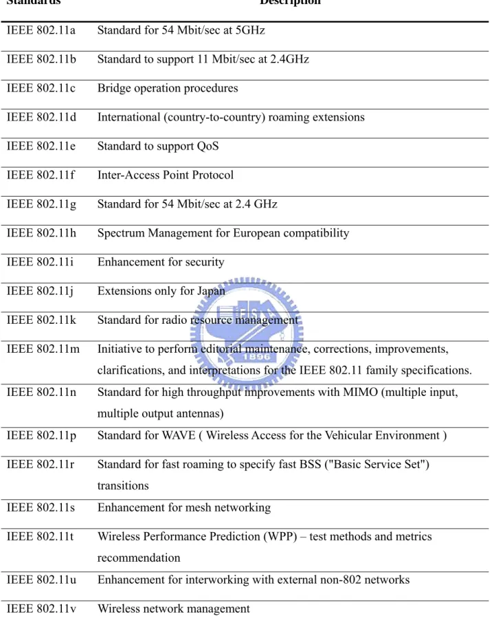
(10) Chapter 1 Introduction. Deployment of wireless networks has grown rapidly in the last decade. It is convenient to connect mobile devices to the Internet without wired line in the public areas, such as libraries, train stations, hotel lobbies, cafeterias, airports, and campus. Nowadays, most of mobile devices such as notebooks, tablet PCs, and PDAs are equipped with one or more wireless communication interfaces. So far, IEEE 802.11 is the most mature and popular protocol amongst other wireless protocols such as Bluetooth, WiMAX, and UWB. The goal of IEEE 802.11 working group established in 1990 is to develop a wireless local area network (WLAN) standard. In 1997, the group approved IEEE 802.11 as the first WLAN standard with data rates of 1 and 2 Mbps only, through three physical medium, infrared (IR), frequency hopping spread spectrum radio (FHSS) and direct sequence spread spectrum radio (DSSS). The IEEE 802.11 MAC sub-layer defines two medium access coordination functions, the base Distributed Coordination Function (DCF) and the optional Point Coordination Function (PCF). Two year later, in 1999, the working group approved two extended WLAN protocol standards. One is 802.11a, it is based on orthogonal frequency division multiplexing (OFDM), operates on U-NII band (Unlicensed National Information Infrastructure) in 5.4GHz, and with a maximum data rate of 54 Mbps. The other is 802.11b, it is based on DSSS, operates in 2.4GHz ISM band, with a maximum data rate of 11 Mbps. The family of IEEE 802.11 is shown in Table 1.1.. 1.

(11) Table 1.1 The IEEE 802.11 family. Description. Standards IEEE 802.11a. Standard for 54 Mbit/sec at 5GHz. IEEE 802.11b. Standard to support 11 Mbit/sec at 2.4GHz. IEEE 802.11c. Bridge operation procedures. IEEE 802.11d. International (country-to-country) roaming extensions. IEEE 802.11e. Standard to support QoS. IEEE 802.11f. Inter-Access Point Protocol. IEEE 802.11g. Standard for 54 Mbit/sec at 2.4 GHz. IEEE 802.11h. Spectrum Management for European compatibility. IEEE 802.11i. Enhancement for security. IEEE 802.11j. Extensions only for Japan. IEEE 802.11k. Standard for radio resource management. IEEE 802.11m. Initiative to perform editorial maintenance, corrections, improvements, clarifications, and interpretations for the IEEE 802.11 family specifications.. IEEE 802.11n. Standard for high throughput improvements with MIMO (multiple input, multiple output antennas). IEEE 802.11p. Standard for WAVE ( Wireless Access for the Vehicular Environment ). IEEE 802.11r. Standard for fast roaming to specify fast BSS ("Basic Service Set") transitions. IEEE 802.11s. Enhancement for mesh networking. IEEE 802.11t. Wireless Performance Prediction (WPP) – test methods and metrics recommendation. IEEE 802.11u. Enhancement for interworking with external non-802 networks. IEEE 802.11v. Wireless network management. 2.

(12) Recently, voice over Internet Protocol (VoIP) became one of the most popular applications. Some products of VoIP, such as Skype, are able to support good quality of voice communication over wired networks. VoIP market grows up quickly due to its low cost and easiness to construct IP network than traditional telecommunication networks. Everyone can use its computer to make cheaper or even free voice call instead of using the expensive cell phone services. According to statistics, it says that the number of residential VoIP users will rise from three million at 2005 to 27 million by the end of 2009 [13]. Therefore, more and more people try to use handheld devices to make VoIP calls through wireless LANs. For this reason, the quality of service (QoS) in WLAN becomes increasingly important. However, voice communication over WLAN features many challenges, such as low bandwidth, large interference, long latency, high loss rates, and jitter. The distributed coordination function (DCF) and the point coordination function (PCF) are unable to guarantee QoS effectively [3], this is because DCF cannot provide QoS trivially, PCF is not efficient for only one frame sent at each polling, point coordinator does not know the QoS requirement of traffic and does not guarantee the delay and jitter bound, so it is harder to provide QoS for real-time audio/video transmission in wireless networks than in wired networks. IEEE 802.11e standard [1] defined at IEEE 802.11 Task Group E is expected to solve the QoS problem of latency sensitive applications over wireless local area networks. 802.11e standard proposes some MAC mechanisms to support time-sensitive applications. Hybrid Coordination Function (HCF) includes two methods, one is Enhanced Distributed Channel Access (EDCA) that combines DCF, and the other is HCF-Controlled Channel Access (HCCA) that is similar to PCF but with enhancement. Direct Link Protocol (DLP) is the option that allows stations to exchange packets directly with other stations, bypassing the AP. Block Acknowledgement, an optional function in implementation, improves channel efficiency by aggregating several acks into one frame. However, IEEE 802.11e is still unable to support satisfactory QoS for time sensitive 3.

(13) applications. EDCA provides QoS based on probability, not determinism. This means, in worst case, the quality of delay time or jitter bound is not desirable. Besides, HCCA polling scheme is not specified in the standard, and the study in [2] shows the HCCA polling overhead problem and its negative effect on the QoS of real-time applications in WLAN. Consequently, a good polling scheme can improve the channel performance and thus QoS for time sensitive applications. Nowadays, the most popular polling scheduler is the round robin (RR) polling scheduler [5] because it is simple in implementation. Many other polling schemes such as [4], [6], [7], [8] have been proposed. In this study, we focus on HCCA polling scheme mainly. We amend a new time-based polling scheduler called Adaptive Time-Stamp Polling (ATSP) scheme. ATSP scheme shows that it can improve total channel utilization and decrease delay jitter variation. In our scheme, Hybrid Coordination (HC) operates at the access point (AP), receives traffic specification (TSPEC) from stations which require polling to send out QoS frames, and records the service start time and maximum service interval corresponding to each station. Then, to avoid polling all stations in turn within one contention-free period (CFP), and using the same service interval for all stations to be polled with different duration of interval, we start to poll a station at its start time of registered service, and the interval for polling this station is same as the interval registered in its TSPEC. By this way, we can reduce the number of polling responded with QoS-Null frame because we don’t poll a station with excessive frequency than its frame sampling frequency, and do not poll a station before it starts communication. In addition, we use a simple mechanism to detect silence mode of a VoIP conversation. Then, we reduced the frequency of polling a silence station in order to decrease unnecessary waste of time. When the station comes back to talk-spurt mode, we revert to the original frequency to poll. The rest of this thesis is organized as follows. Chapter 2 introduces the background of 802.11, 802.11e, voice/video transmission characteristic, and a brief survey of current polling 4.

(14) mechanisms. In Chapter 3, we discuss the proposed polling mechanism in detail. In Chapter 4, simulation and numerical results are demonstrated. Finally, the conclusion and future works are presented in Chapter 5.. 5.

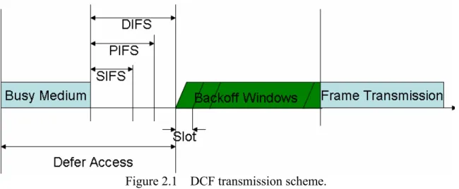
(15) Chapter 2 Background and Related Work. In this chapter, we will review IEEE 802.11 MAC, including DCF and PCF. Next, we review IEEE 802.11e, including how EDCA and HCCA work. Then we will give a brief of the advantages and disadvantages of WLAN MAC mechanisms. Furthermore, we will go through the attributes of multimedia transmissions and how their codec work. Finally, we will list some related works that have been proposed.. 2.1 Review of IEEE 802.11 MAC Access to the wireless medium is controlled by coordination functions. 802.11 defines two different basic exchange procedures. One is the distributed coordination function (DCF) which is used in contention-based services; the other is the point coordination function (PCF), if contention-free service is required. Contention-free services are provided only in infrastructure networks. The coordination functions are described as follows.. 2.1.1 Distributed Coordination Function DCF is a fundamental function in IEEE 802.11 protocol. It is the basis of the standard Carrier Sense Multiple Access with Collision Avoidance (CSMA/CA) access mechanism with binary slotted exponential backoff. Like Ethernet, when a station needs to send packets, it first checks to see whether the channel is clear before transmitting. If the channel has been idle for longer than DCF Interframe Space (DIFS), the station will try to transmit packets. If the channel is busy, the station should wait for the channel to become idle for DIFS and prepare for the exponential backoff procedure in order to avoid collisions. 802.11 refers to the wait as access 6.

(16) deferral (see Fig. 2.1).. Figure 2.1 DCF transmission scheme. The backoff window is divided into slots. Slot length is medium-dependent, generally, higher speed physical layers use shorter slot times. During the backoff procedure, station picks a random number of slots from contention window size. In other words, after a packet transmission was completed and DIFS has elapsed, several stations attempt to transmit again, the station that picks the lowest random number of slots wins.. Figure 2.2 DSSS contention window size. Contention window sizes are always a power of 2 minus 1 (e.g., 31, 63, 127, 255). The size of the contention window depends on the physical layer. For example, the DS physical layer limits the contention window to 1023 transmission slots, and after each unsuccessful transmission, 7.

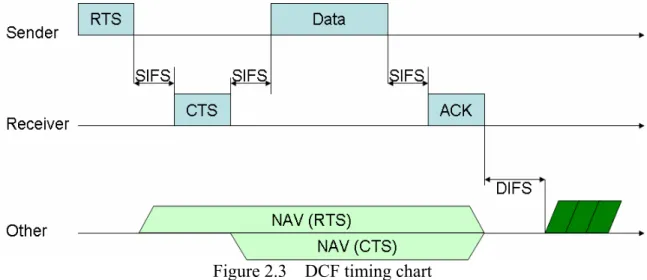
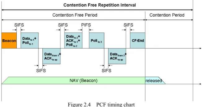
(17) the contention window moves to the next greatest power of two (see Fig. 2.2) until it reaches the limit. Furthermore, with hidden nodes problem, RTS/CTS exchange procedure is an optional scheme. The sender transmits a request-to-send (RTS) packet before data frame transmission, and the receiver answers a clear-to-send (CTS) packet. RTS and CTS packets include information called network allocation vectors (NAV), station will set NAV to the time that it expects to use the medium. Then, other stations count down from NAV to 0. When the NAV reaches 0, it means that the channel is idle (see Fig. 2.3). Since this scheme may generate huge overhead when data packets are small, RTS/CTS is introduced for only those packets whose sizes larger than a certain threshold.. Figure 2.3 DCF timing chart. 2.1.2 Point Coordination Function The PCF is an optional access mechanism of the 802.11 specification, it is a centralized scheme which uses the AP as a point coordinator (PC). When the PCF is enabled, time on the channel is divided into the contention-free period (CFP) and the contention period (CP). The periods of contention-free service and contention-based service repeat at regular time intervals, which are called the contention-free repetition interval. In order to prevent interference, all 8.

(18) transmissions in contention-free period are separated by the short interframe space (SIFS) and the PCF interframe space (PIFS). Since SIFS and PIFS are shorter than DIFS, DCF-based stations can not gain access to the medium using the DCF. When a station is polled, it starts to send a data frame after SIFS, according to the specification, each poll is a license to send only one data frame. Multiple frames can be transmitted only if the access point sends multiple poll requests. To make sure that the point coordinator owns control of the channel, it may poll the next station on its polling list if there is no response after an elapsed PCF interframe space (see Fig. 2.4).. Figure 2.4 PCF timing chart To improve efficiency, ACK, polling, and data transfer in the contention-free period may be combined, for example, Data+CF-Poll, Data+CF-ACK, Data+CF-Ack+CF-Poll, etc. And, the contention period must be large enough for the transmission of at least one maximum-size frame plus an ACK. When the contention-free period begins, the access point transmits a beacon frame. The beacon will announce the maximum duration of the contention-free period. All stations receiving the beacon would set the NAV to the maximum duration to avoid DCF-based access to the wireless. If the existing frame exchange will occupy the contention-free period, it is allowed to 9.

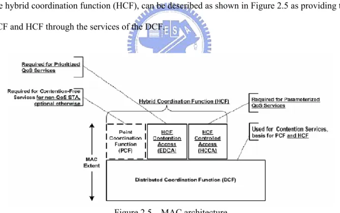
(19) complete the transmission. Then, the AP transmits a beacon frame to announce the start of the contention-free period. The contention-free period is shortened by the amount of the delay. The point coordinator may also terminate the contention-free period before its maximum duration by broadcasting a CF-End frame.. 2.2 Introduction to IEEE 802.11e The IEEE 802.11e defines the medium access control (MAC) procedures to support applications with quality of service (QoS) requirements, including the transport of voice, audio, and video over IEEE 802.11 wireless LANs (WLANs). The architecture of the MAC sublayer, including the distributed coordination function (DCF), the point coordination function (PCF), and the hybrid coordination function (HCF), can be described as shown in Figure 2.5 as providing the PCF and HCF through the services of the DCF.. Figure 2.5 MAC architecture The HCF uses both a contention-based channel access method, called the enhanced distributed channel access (EDCA) mechanism for contention-based transmission and a controlled channel access, called the HCF controlled channel access (HCCA) mechanism for contention-free transmission. 10.

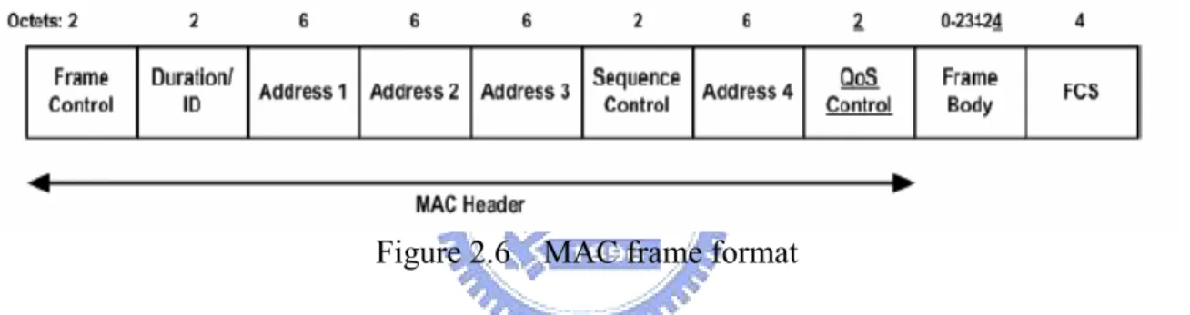
(20) Stations that implement the 802.11e facility may obtain transmission opportunity (TXOP), which is an interval of time that station has the right to initiate frame exchange sequences on the wireless channel. A TXOP is defined by a starting time and a maximum duration, and the station that has obtained TXOP by successfully contending for the channel or assigned by the hybrid coordination (HC) can transfer one or more frames on the channel until the duration is over. Each QoS data frame in 802.11e consists of a QoS control information, Figure 2.6 shows the 802.11e MAC frame format. The QoS Control field identifies that the traffic category (TC) or traffic stream (TS) which the frame belongs to and other QoS information, for example, the information about the corresponding MSDU, limit of TXOP, TXOP duration requested, ACK policy, etc.. Figure 2.6 MAC frame format In the following list, we will describe the major coordination function of 802.11e MAC architecture, the Enhanced Distributed Channel Access (EDCA) and the HCF-Controlled Channel Access (HCCA), and how they work to implement QoS requirement in detail.. 2.2.1 Enhanced Distributed Channel Access (EDCA) The EDCA mechanism defines four access categories (ACs) that provide support for the delivery of traffic with user priorities (UPs) at QoS stations (QSTAs). Voice, video, best-effort and background traffics are mapped into these four ACs. The ACs are used to contend for the channel in order to transmit data frames with certain priorities and are derived from UPs as shown in Table 2.1. Unlike DCF mechanism whose contention is between stations, in EDCA 11.

(21) mechanism, each AC behaves as a single DCF contending entity and each AC has a corresponding parameter set. In fact, data frames are classified into four different FIFO queues in accordance with ACs (see Figure 2.7). Table 2.1 UP-to-AC mapping.. Fig. 2.7. Reference implementation model. For each AC, EDCA assigns different arbitration interframe space (AIFS), minimum contention window size (CWmin), maximum contention windows size (CWmax) and TXOP duration. Those parameter sets are announced by the AP periodically via beacon frames. It assigns smaller CWmin, CWmax and AIFS to ACs with higher priorities in order to bias the success probability that the QoS data frames can be sent with smaller delay. EDCA uses a new 12.

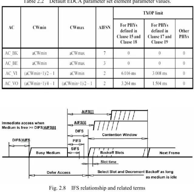
(22) type of interframe space called AIFS, it is an time interval with arbitrary length and determined by the following equation, AIFS[AC] = AIFSN[AC] * aSlotTime + aSIFSTime. The parameter set is shown in Table 2.2. In 802.11e standard, the value of AIFSN[AC] of QSTAs must be greater than or equal to 2, and the value of AIFSN[AC] of QoS access points (QAPs) must be greater than or equal to 1. Generally, AIFSN of AC_VI and AC_VO (see Table 2.2) for QAPs are set to 1, others for QAPs are same as that in Table 2.2, and DIFS = 2*aSlotTime + aSIFSTime. It means that AIFS of AC_VI and AC_VO is equal to DIFS for QSTAs, and AIFS of those is less than DIFS for QAPs. For this reason, the QAPs can transfer video and voice data frames with highest probability and the QSTAs transfer video and voice with second highest probability. 802.11e defines a TXOP limit as the interval of time during which a station has the right to initiate transmissions. The TXOP limit duration is introduced by the QAP as information element in the EDCA parameter set of beacon frames and probe-response frames. During a TXOP, stations can transmit one and more data frames from the same AC with a SIFS time between an ACK and the following data frame. A TXOP limit value of 0 means that a single MSDU only, in addition to a possible RTS/CTS frames exchange or CTS frame to itself, can be transmitted during each TXOP. Figure 2.8 illustrates these EDCA parameters and the access procedure. Before each AC tries to send frames onto wireless channel, it needs to wait for an idle interval time of AIFS[AC], and a random backoff time from its corresponding CW. The purpose of different contention parameters for different queues of ACs is to give high-priority traffic more chances to gain the right to use the channel. The end of backoff times of different ACs in one station may be the same sometimes, this situation will cause internal collisions and reduce the efficiency of service. In order to avoid these internal collisions, EDCA establishes a virtual layer inside MAC layer (see Fig 2.7) to allow the higher priority AC to send frames earlier. Therefore, the EDCA can support prioritized QoS for 13.

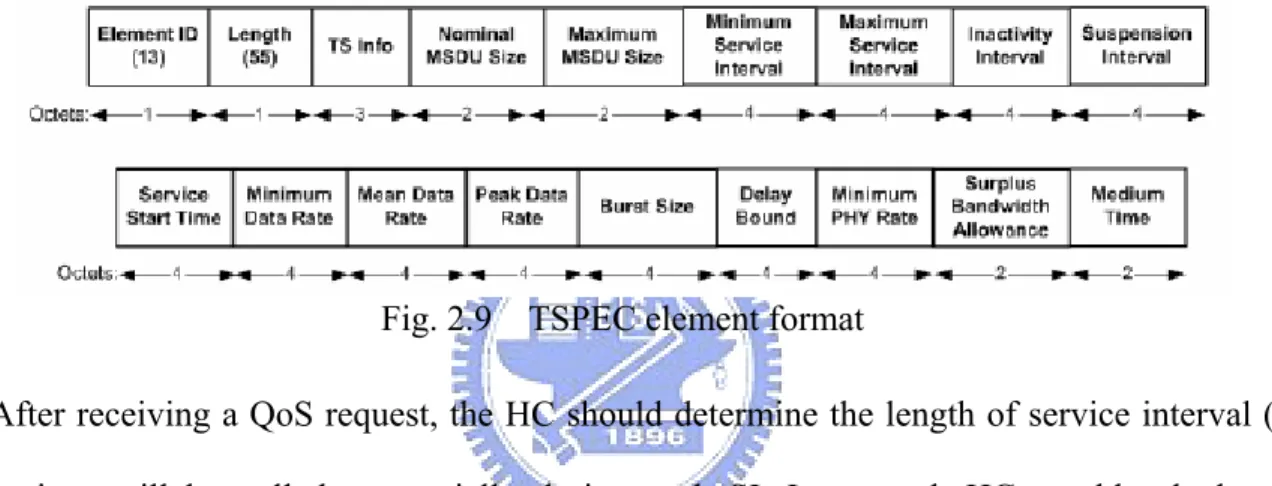
(23) time-sensitive audio/video applications. Table 2.2 Default EDCA parameter set element parameter values.. Fig. 2.8. IFS relationship and related terms. 2.2.2 HCF Controlled Channel Access (HCCA) The HCCA mechanism manages access to the channel, using an AP as hybrid coordinator (HC) that has higher access priority than stations. An AP can poll stations during contention free period (CFP) and contention period (CP). But in traditional PCF, polling is only allowed during CFP. This makes HCCA more flexible. During a CP, an AP is able to obtain the control of the channel for a certain time period, called controlled access phase (CAP), in order to poll multiple 14.

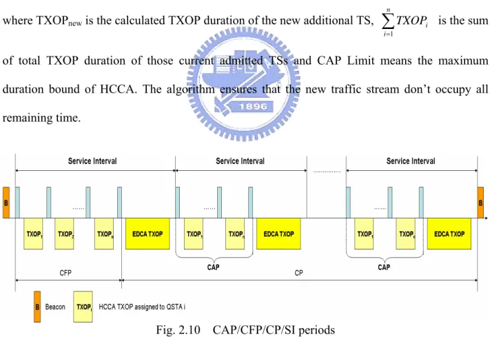
(24) stations after sensing the channel to be idle for a PCF interframe space (PIFS). The AP has higher priority to start CAP and polling during CP because PIFS is shorter than DIFS and any AIFSs. In HCCA, each QSTA which wants to be polled for QoS support must register a traffic stream (TS) to the HC by delivering the QoS parameter values in a particular traffic specification (TSPEC). The TSPEC includes information about the TS, such as mean data rate, delay bound, and maximum service interval (see Fig. 2.9). Then, QAP needs to provide services that conform to the demands registered in the TSPEC under controlled operating condition if this QAP admitted it and established the TS.. Fig. 2.9. TSPEC element format. After receiving a QoS request, the HC should determine the length of service interval (SI), and stations will be polled sequentially during each SI. In general, HC would calculate the smallest one among all maximum service intervals for those accepted TSPECs. Let the chosen one be SImin. Then, HC chooses a value smaller than SImin and this value should be a sub-multiple of the beacon interval. This value is the final SI for all QSTAs and admitted traffic streams, in this way, the beacon interval would be cut into several service intervals. Figure 2.10 shows the relationship of the CAP, CP, CFP and SI. After HC calculated the SI for HCCA mechanism, it will also calculate the TXOP for those admitted TSs. First, HC calculates the number of frames that will arrive at the mean data rate. ⎡ SI * ρ i ⎤ during an SI by Ni = ⎢ ⎥ , where Ni is the number of frames sent from the stream i during ⎢ Li ⎥ an SI, ρi is the mean data rate for stream i and Li is the nominal MSDU size of stream i. Then HC 15.

(25) ⎛ N * Li ⎞ M + O, + O ⎟⎟ , where TXOPi is the polled calculates the TXOP duration by TXOPi = max ⎜⎜ i Ri ⎝ Ri ⎠ TXOP duration of stream i, Ri is the physical transmission rate, M is the maximum MSDU size and O refers to the transmission overheads. By using those calculated TXOPs, we can make a simple admission control algorithm. The algorithm is to make sure that the sum of total TXOPs duration must be less than a CAP upper bound. When a new TS wants to be added into the HCCA polling list, it must meet the following equation, n. TXOPnew + ∑ TXOPi i =1. SI. ≤. CAP Limit Beacon Interval. ,. …………………………………………….(2.1). where TXOPnew is the calculated TXOP duration of the new additional TS,. n. ∑ TXOP i =1. i. is the sum. of total TXOP duration of those current admitted TSs and CAP Limit means the maximum duration bound of HCCA. The algorithm ensures that the new traffic stream don’t occupy all remaining time.. Fig. 2.10 CAP/CFP/CP/SI periods However, this algorithm for calculating TXOP assumes all traffic streams are in constant bit rate. In practice, lots of real-time applications, such as VoIP or video conference, are using variable bit rate. So it may cause the queue overflow and packet drop that decreases the level of 16.

(26) QoS.. 2.3 Summary of WLAN MAC Mechanisms Two WLAN MAC mechanisms defined in IEEE 802.11 and 802.11e had been discussed in the previous chapter. One is contention-based, such as DCF and EDCA, and the other is contention-free-based (poll-based), such as PCF and HCCA. These two types of MAC mechanism have their own advantages and disadvantages, and we address them in this section. The contention-based mechanism has several advantages. DCF and EDCA have a lower complexity of implementation than the contention-free-based mechanism which includes PCF and HCCA. Furthermore, contention-based mechanism is adaptive to dynamic change of traffic load and network condition. However, when more and more QSTAs enter the same channel, the waiting time of QoS data transmission may become longer and longer. This type of mechanism has hidden node problems that may cause extra collisions. The main drawback is that contention-based mechanism cannot guarantee QoS because it uses random backoff for QoS provisioning. It means probability takes the place of guarantee. Further, the backoff time is another overhead. There are several advantages in contention-free-based mechanisms. The first advantage is the higher dependability on supporting QoS because it uses contention free transmission and centralized control mechanism on AP. It also can eliminate the hidden node problems. The channel utilization might be better than contention-based in the same situation because it reduces backoff time and collision overhead. Nevertheless, the complexity of implementing contention-free-based mechanisms is much higher than contention-based mechanisms since AP needs to schedule the sequence of QSTAs and might need to calculate transmission time. Furthermore, the excessive polling overhead is a critical problem if AP polls a station which has no QoS data frame in queue. 17.

(27) 2.4 Attributes of Real-Time Multimedia Transmissions We will introduce attributes of voice and video traffics briefly in this section, these include the packet duration, required bandwidth, the characteristics of those traffic streams. It shows that there are many voice and video requirements for the channel capacity over the wireless LANs. First we discuss voice traffic, referring specifically to VoIP. Most applications of VoIP generate variable bit rate (VBR) traffic, this means that they generate packets only when the users of those applications are talking. Less applications of VoIP generate packets at constant bit rate (CBR), it means that they generate packets continuously with constant interval, 10ms, 20ms, 30ms, etc. Every VoIP codec might have different packet intervals and different transmission frequencies in Table 2.3 no matter it is CBR or VBR.. Codec. ITU-T G.711. ITU-T G.723.1 ITU-T G.726 ITU-T G.728 ITU-T G.729A GSM 06.10. Table 2.3 VoIP codec standards Bit Rate Payload Packet per Second (kbps) (bytes) (pps) 80 100 64 160 50 240 33.3 24 33.3 6.4 30 25.96 20 33.3 5.3 30 22.2 32 120 33.3 16 60 33.3 20 50 8 30 33.3 13 33 20. Packet Duration (ms) 10 20 30 30 38.5 30 45 30 30 20 30 50. It will cause extra polling overhead when the AP chooses the smallest one among all maximum service intervals as the final service interval for the AP to poll QSTAs (see Chapter 2.2.2). For example, there are two VoIP applications with different service intervals 20ms and 50ms, AP will poll both stations every 20ms. Hence, for the station with service interval 50ms, it should return QoS data frames 20 ( 1000 / 50 = 20 ) times after AP polls it within 1000ms, but actually it will be polled 50 times. This causes 30 useless pollings which waste time. In 802.11b 18.

(28) wireless LAN, we assume that the physical overhead is 192µs, SIFS is 10µs and CF-Poll frame transmission is at the basic rate (2 Mbit/sec) regardless of the data rate, and QoS-Null frame is transmitted at the maximum physical data rate (11 Mbit/sec), then we ignore the packet propagation time because this time is only few microseconds. So the time wasted would be. 30 × {(192 + 36 × 8 ÷ 2) + 10 + (192 + 36 × 8 ÷ 11)} ÷ 1000 ≈ 17 ms in every 1000ms. According to Table 2.3, we also can see that VoIP requires relatively low bandwidth, the VoIP packet transmission frequency is very high and the payload size of voice traffic packets is smaller than other type of packets. Furthermore, it usually causes greater transmission overhead in VoIP than in general data transmission. For example, in G.711 over 802.11b wireless LANs, it needs 192µs for physical overhead duration, 52bytes for UDP, IP and MAC headers cost 38µs, and average backoff time is CW min ÷ 2 × Slot Time = 32 ÷ 2 × 20 = 320 μs whereas only 116µs is required to transfer a pure VoIP payload of 160bytes. In contention-free period based on polling mechanism, it still costs 336µs to transmit a CF-Poll frame instead of backoff time. Only about. 116 (192 + 38 + 320 + 116) × 100% ≅ 17.42% of transmission time is used to transfer VoIP data even we use low rate VoIP codec at 802.11b wireless LANs. The main attribute of voice transmission application is the alternation of talk-spurt and silence, that means users would stop talking and just listen to others sometimes, then they restart to talk later. This alternation is independent of the codec and application. If the voice application is VBR, during talk-spurt period the voice source works as isochronous source with stable interval time which is defined by the voice codec, and the voice source does not generate any voice frames during silence period. This attribution of voice transmission makes the original round robin (RR) polling schedule not efficient at all. This is because that the AP will not stop to poll VoIP stations which are in silence period. The AP continues to poll those VoIP stations even they respond no frame every time. It causes waste of bandwidth and increases unnecessary delay to other traffic streams. 19.

(29) Similarly, in video codec, there are several specifications, such as popular MEPG-1/2/4/7 standards defined by ISO and promising H.263 and H.264 standards defined by ITU-T. Video codecs have different sampling rates and intervals. For this reason, there might be lots of video transmissions with different service intervals in the same channel. Same as voice codec, it will still cause extra polling overhead when an AP chooses the smallest one amoung all maximum service intervals as the final service interval to poll QSTAs. Nevertheless, the payload size of video packet is usually up to 1000Bytes and most video streams do not have talk-spurt and silence alternation. So they cause less problem than voice streams.. 2.5 Related Works In our survey, most of those enhanced EDCA schemes tend to adjust the contention parameters of EDCA, for example, CWmin, TXOP duration, AIFS length. Some schemes try to change CWmin and AIFS length for the design of each AC such as that in [21], and some change those parameters dynamically according to the network condition such as traffic load [22]. Other adaptive schemes are focusing on adjusting the process of random backoff in contention depending on the network utilization or the priority of each AC such as that in [20]. In conclusion, the main improvement scheme of EDCA is to find better parameters for CWmin, AIFS length and etc, then let the frames of higher priority of AC be sent sooner and sooner. For those enhanced polling schemes, there are fewer researches about HCCA than EDCA. Those adaptive schemes for HCCA usually try to find a mechanism to solve polling those stations without data frame ready in order to reduce the polling overhead. In [6], HC increases the polling interval of those stations that do not respond data frame to decrease the total polling overhead. In [9], AP will stop polling those stations which are considered silence stations, and increase the priorities of those stations during contention periods, and start to poll when they transmit QoS frames again. In [10], the VBR traffics and CBR traffics are transmitted in 20.

(30) contention periods and contention-free periods respectively, this means AP only polls stations with CBR traffic. Another improvement schemes of HCCA focus on adjusting the TXOP duration to make polling process fairly. In [11], the determination of TXOP duration depends on TSPEC and current traffic status. Admission control is important for AP to support QoS. Nowadays, there are two kinds of suggested admission control methods. One is that the AP measures the network condition continuously. To accept or deny a QoS request is based on the current throughput, average delay or other estimations. The other method is that the AP constructs a certain performance metric to forecast the status of the network and decide whether the QoS request is accepted or not. However, since there are a lot of interference factors which are difficult to be handled, the research of admission control in WLAN is still an active topic of study.. 21.

(31) Chapter 3 Proposed Polling Scheme. In the previous chapter, the traditional round-robin polling scheme is not efficient for VBR traffic streams due to talk-spurt and silence alternation, and it causes large polling overhead because it uses the same service interval for all QoS traffic streams with requested different service intervals. Whether the AP polls the stations during silence periods or polls those stations with shorter service intervals than its actual frame intervals, both events will result in large polling overhead. Unnecessary overheads will decrease the channel utilization, raise the packet access delay, and influence the deviation of jitter. If we want to provide higher quality of service for voice and video streams, we need a more efficient polling scheme that can avoid polling those stations which might not respond any data. In this chapter, we propose an adaptive time-stamp poll scheming based on HCCA to provide better QoS in wireless LAN environment, and its associated auxiliary mechanisms that detect the silence periods and reduce the access delay. This scheme is able to reduce the number of unnecessary polling but not degrade the requested QoS, and the scheme operates on the top of MAC layer in the AP to manage the polling schedule and mitigate the access delay and jitter of those QoS traffic streams. First, we will introduce our proposed scheme and explain how it works in detail. Then we discuss all kinds of situation that may happen in our proposed scheme and show how we handle them. We also rehearse this scheme by presenting some examples to compare it with round-robin polling scheme.. 22.

(32) 3.1 Main Architecture The key idea of our proposed scheme is that HC calculates more suitable time to poll those traffic streams. The HC does not poll all traffic streams in the polling list during one CAP because each traffic stream has its own service start time, and requires a different service interval. So we propose an adaptive time-stamp poll scheduling which tries to calculate fairer and more efficient polling time for each traffic stream. After the HC calculates the suitable polling time, it polls those traffic streams exactly at their own calculated polling time. However, only using this schedule is not sufficient for QoS of real-time applications. Therefore, we use a shorter interval to poll some traffic streams at the beginning of their transmission during a very small period, called the short interval polling function, in order to reduce the access delay. We also endeavor to solve the talk-spurt and silence problem of voice traffic streams such as VoIP. When a traffic stream has not generated data frames for a while, we use a simple count of receiving QoS-Null frames to determine whether it enters into silence mode or not. Figure 3.1 shows an AP decision flow. When the current time equals or exceeds the calculated polling time, the HC sends a CF-Poll frame for this traffic stream. After it responds, the HC calculates the next polling time by adding different intervals depending on its current situation as shown in Figure 3.1. Our proposed polling scheme does not modify the 802.11e standard; we do not need to add any new frame type. It enhances the original HCCA protocol with better poll scheduling policy. In the following, we will focus on those mechanisms mentioned previously in detail. We present adaptive time-stamp poll scheduling in Section 3.2 and show its advantages. In Section 3.3, we introduce the short interval polling function. And we show how we solve the talk-spurt and silence alternation problem in Section 3.4.. 23.

(33) Fig. 3.1. AP decision flow chart. 3.2 Poll Scheduling Mechanism. 3.2.1 Time-Stamp Poll Scheduling We propose an adaptive time-stamp poll scheduling method, the method starts to poll a new QoS station at its service start time which is registered in the accepted TSPEC (see Fig. 2.9). The service start time of a TSPEC means the time this QoS traffic stream needs the HC to poll it for transferring QoS data frame. Sometimes the original HCCA or PCF methods will start to poll the stations before their service start time because it tends to poll all accepted QoS traffic streams in a single contention-free period (CAP). It usually wastes time because these streams may not be 24.

(34) ready to send frames. In order to avoid such time consumption, when a new traffic stream’s QoS request is accepted, the HC starts to poll those stations exactly at its service start time. When a QoS traffic stream has been polled, the HC calculates the next time to poll this stream by adding the maximum service interval in the TSPEC of this stream. Unlike original HCCA method, it uses adaptive polling intervals to each traffic stream instead of the unitary service interval. We do not use very small intervals to poll stations, instead we use maximum service intervals of them, so as to avoid unnecessary polling. Our basic polling time calculation formula is as follows: 1st PollingTim ei = ServiceSta rtTime i ,. ....…………………………………………........ (3.1). 2 nd PollingTim ei = 1st PollingTim ei + MaximumSer viceInterval i , ……………………….(3.2) n + 1th PollingTim ei = n th PollingTim ei + MaximumSer viceInterval i , ………………….(3.3). where PollingTimei is the predetermined time in which the traffic stream i will be polled, and MaximumServiceIntervali is the maximum service interval specified in the TSPEC of the traffic stream i. In general, every HC has a clock to provide current time. When one of the polling time of a traffic stream is encountered, the HC tries to poll this traffic stream to give the temporal ownership of the channel to this stream for transmission. However, in some special case that we would discuss later, the HC can not poll these stations at their expected polling time exactly but delay for a while. In such situation, the HC should endeavor to poll this postponed traffic stream as soon as possible because it has passed the exact polling time. The method of polling stations and exchanging frames during TXOP duration in our adaptive time-stamp scheme is same as the one in the original 802.11e HCCA scheme. When the HC detects that the present time equals to one of expected polling time of those traffic streams, the HC first checks to see whether the channel is clear before transmitting. If the channel is busy, the HC should wait for the channel to become idle for PCF Interframe Space (PIFS). If the 25.

(35) channel has been idle for longer than PIFS, the HC sends CF-Poll for this assigned traffic stream to provide ownership and calculated TXOP duration. Both the HC and the station which had been polled would exchange frames with combining ACK, data or polling types at interval of SIFS. If there is no data frame to transmit by this traffic stream before the end of TXOP duration, the HC sends the CF-End frame to all stations and comes back to the contention modes. And if there is one or more expected polling time occur among the current TXOP duration, the HC do not halt the current TXOP. The HC would poll these traffic streams just following the termination of the present TXOP duration by transferring Data+CF-ACK-CF-Poll frames or CF-Ack+CF-Poll frames like the method of HCCA. In traditional round-robin poll scheduling of HCCA mechanism, it chooses the smallest service interval among all maximum service intervals of those accepted traffic streams as the interval in which the AP polls all stations as described in Section 2.2.2. However, it will cause extra polling when it uses a shorter service interval than that the station really needs.. Fig. 3.2. Illustration of traditional RR polling scheme. For example, there are three stations which need to be polled for QoS transmission in HCCA method, station 1 requests polling with a maximum interval of 20ms that equals to the duration it 26.

(36) generates the video or voice frames. Similarly, station 2 requests polling with a maximum interval of 30ms, station 3 requests polling with a maximum interval of 50ms and the beacon interval is 100ms. The hybrid coordinator (HC) will choose 20ms as the final service interval to start contention-free periods or controlled access phases (CAPs). During contention-free periods, all QoS-requested stations to be polled by the HC will be polled certainly in proper order. Figure 3.2 is an illustration for the previous example. After the beacon, it will start the contention-free period to poll three stations in turn, then after a service interval of 20ms, it starts the CAP to poll those stations one by one again, and it repeats every 20ms. This means that the HC polls all three stations every 20ms regardless of the true intervals in which those stations generate their video or voice frames actually. Therefore, station 2 generates QoS data frame in 30ms but is polled every 20ms and station 3 generates frames every 50ms; both of them will no doubt respond the QoS-Null frames after certain times of polling. It causes extra polling overheads and decreases the channel utilization.. Fig. 3.3. Illustration of adaptive time-stamp polling scheme. However, the previous problem will be overcome in our proposed adaptive time-stamp 27.

(37) scheme. For the same example, station 1 is polled at a maximum interval of 20ms, station 2 is polled at a maximum interval of 30ms, and station 3 is polled at a maximum interval of 50ms. They start to be polled at their own service start time with different service intervals. Figure 3.3 is an illustration for the same example using our proposed scheme. It looks like no contention-free periods, but the HC polls all stations during CAPs in contention periods. Each CAP period contains one or more polled TXOPs in accordance with the actual needs. In this illustration, there are some polled TXOP delays for station 1 and 2, because the polled TXOP duration of station 3 extends to the polling time of station 1, and in turn the TXOP of station 1 extends to the polling time of station 2. As Figure 3.2 and Figure 3.3 demonstrated, our proposed polling method can avoid unnecessary polling and improve the channel utilization.. 3.2.2 Polling Policy and Priority We address the scheduling policy and priority of polled TXOP in this section. As discussed in the previous chapter, the HC may not be able to poll certain station exactly at its intended polling time because the channel is not idle at that time. In this case, the HC should reschedule the polling of this traffic stream immediately. Here we will present all possibilities in detail. To start, no matter what was the reason of delay, the HC still needs to wait for one PIFS time to see whether the channel is clear before transmitting, then the HC could send a CF-Poll frame to poll a traffic stream. In our adaptive scheme, the contention function is same as 802.11e EDCA standard which was introduced in Section 2.2.1. It means, the best-effort data transmission could be sent just one frame at every successful contention, and both the voice and video data frames exchange between the AP and the QSTAs uses SIFS as intervals during EDCA TXOP durations. Similarly, the data exchange during a polled TXOP duration also uses SIFS as intervals. Consequently, the HC must not hold any current TXOP to poll any deferred traffic stream. If 28.

(38) being delayed by voice or video frames, the deferred polling must wait until the total TXOP duration finishes because SIFS is smaller than PIFS. If it is delayed by best-effort frames, the deferred polling just waits one data frame, one SIFS and one relative ACK because PIFS is smaller than DIFS. The reason is not only the interval length but also that EDCA TXOP is as important as polled TXOP, and best-effort data transfer is less urgent. Suppose that there is a lot of polled TXOP durations which had been delayed, how could we reschedule multiple deferred TXOP durations. The method we proposed in our adaptive scheme is to poll those traffic streams sequentially in accordance with the order of the intended polling time. With this method, it can avoid excessive and aggregate delay in some particular traffic stream. In the worst case, if all expected TXOP durations have been delayed during the same time, the HC needs rescheduling all TXOP duration sequentially. The outcome will be the same as the original round-robin polling scheme and it will not make other unnecessary delay.. 3.2.3 Jitter Deviation Reduction For voice and video traffic streams, the jitter deviation is very important for the QoS applications. If the deviation of jitter is large, it means the frame inter-arrival time of this traffic stream varies seriously and this event will make users uncomfortable because the voice or video traffic streams might intermit randomly. So we need to minimize the jitter deviation to supply better QoS. Our adaptive time-stamp polling scheme can reduce the deviation of jitter easily. In general, the packet generating duration of the traffic stream will be the same as the maximum service interval registered in the TSPEC. For example, the traffic with the codec G.726 (see Table 2.3) will generate packets every 30ms and the maximum service interval in registered TSPEC is 30ms. The HC will poll this traffic stream every 30ms. While the polling interval of this traffic stream is the same as the interval with which the frame of this stream is generated, the jitter deviation will 29.

(39) be very small and stable.. Fig. 3.4 Illustration of nth polling with responding data. Fig. 3.5. Illustration of polling with responding mth data. We use mathematical equations to express this jitter deviation reduction in our proposed scheme. Since we can not confirm whether the service start time equals to the first packet generating time, so we assume that the HC got response with data frames at first time in nth polling, and the latest one of those transferred frame is the mth frame generated (see Fig 3.4 and 3.5). Then we consider the jitter barely between the QSTAs and the AP. The equations about transmission time and access delay are as follows: TransmissionTime = AccessDelay + PropagationDelay,. ……………………………(3.4). where propagation delay means the time of frame propagation in channel and is the same for the frames in the same traffic stream. The access delay is the time that the frame in queue waits to be 30.

(40) transmitted. 1st AccessDelay = nth PollingTime + Overhead1 – mth FrameArrivingTime, ……………(3.5) 2nd AccessDelay = n+1th PollingTime + Overhead2 – m+1th FrameArrivingTime,. …(3.6). 1+ith AccessDelay = n+ith PollingTime + Overheadn+i – m+ith FrameArrivingTime, …(3.7) where polling time is calculated by Equation 3.1, 3.2 and 3.3. Frame arriving time means the time at which the frame was ready and arrived at queue, and overhead is the sum of the delay caused by other frames or TXOP duration, CF-Poll transmission time, inter-frame space before data frame transmission and other delays. The jitter means the difference of the transmission times of the adjective frames, and the equations about jitter in our proposed scheme are as follows: 1st Jitter = 2nd TransmissionTime – 1st TransmissionTime = ( 2nd AccessDelay + PropagationDelay ) – ( 1st AccessDelay + PropagationDelay ) = 2nd AccessDelay – 1st AccessDelay = ( n+1th PollingTime + Overhead2 – m+1th FrameArrivingTime ) – ( nth PollingTime + Overhead1 – mth FrameArrivingTime ) = ( n+1th PollingTime – nth PollingTime ) + ( Overhead2 – Overhead1 ) – ( m+1th FrameArrivingTime – mth FrameArrivingTime ) = PollingInterval + ( Overhead2 - Overhead1 ) – FrameInterval = Overhead2 – Overhead1 ,. …………………………………………………(3.8). nth Jitter = Overheadn+1 – Overheadn , …………………………………………………(3.9) where the polling interval is the same length as the frame arriving interval in our proposed scheme for identical traffic stream, this is the reason why we can cancel polling interval and frame interval out at Equation 3.8. From Equation 3.9, we know the general jitter comes from the overhead difference of adjacent frames. The adjacent overhead difference comes mainly from the delays caused by other 31.

(41) frames or TXOP duration. However, the length of this delay is no more than the sum of single EDCA TXOP duration and all polled TXOP duration minus one polled TXOP duration, but the probability of this case is very little. This is because the polling start time and the service intervals of different traffic streams are varied. For this reason, the overheads are usually little, also the differences of the adjacent overheads are very little. Therefore, we proved that the jitter deviation in our adaptive time-stamp polling scheme will be smaller than that in original RR polling scheme based on mathematical analysis as discussed in this section.. 3.3 Access Delay Reduction We can know the access delay of the preceding frame is very close to the access delay of the following one in the same traffic stream if we subtract the access delays (see Equation 3.7) of those adjective frames such as that in the following equation: i + 1th AccessDela y − i th AccessDela y = Overhead n + i +1 − Overhead n + i , ……………...... (3.10). we can easily understand that the difference of those adjective access delays will be close to zero, this means that access delays will be vary stable because most of the overheads are very small. However, if there was one QoS traffic stream that transmits first frame with much higher access delay, the access delay of its succeeding frames may be high accordingly.. 3.3.1 Relationship of Frame Arriving Time and Access Delay Assuming the access delay of the frame is the waiting time for transmission in the queue, and the frame arriving time is its arrival time at queue and is ready to be sent. So the average access delay would be decided by the difference of the frame arriving time and the relative polling time. 32.

(42) Fig. 3.6. Relationship of frame arriving time and access delay. As Figure 3.6 shows, there are three dotted lines, each represents one situations. If the QoS traffic stream starts before the service start time, the average access delay will be close to the access delay a. If it starts after the service start time, the average access delay will be close to the access delay b. Since the frame arriving time is not under control by the HC, the average access delay may be up to its polling interval. For example, there is a traffic stream with registered polling interval of 100ms, it may have an average access delay up to 100ms. This issue will be enlarged when the traffic streams have large polling intervals.. 3.3.2 Short Interval Polling Function In order to reduce the average access delay of each traffic stream, we propose a short interval polling function, which is able to reduce the access delay down to less than an artificial number. If we choose 10ms as the short interval for this function, the access delay won’t be more than 10ms. The function is that the HC polls the traffic stream with its short interval after it polled this traffic stream, and was replied QoS data frames at the first time. For example, as Figure 3.7 shows, the original polling interval is much longer than the defined short interval, and the HC 33.

(43) received the first QoS data frame at nth polling. Then the HC starts the short interval polling function to poll this traffic stream at short interval. So the new access delay will be less than the short interval and may be much less than the old access delay.. Fig. 3.7 Illustration of short interval polling function We do not worry about traffic streams in silence mode at the beginning that may interfere this short interval polling function because the HC executes this function only after it received QoS data frames at the first time. It could reduce the possibility that the HC was replied QoS-Null frames for a long time in short interval polling function. However, if there really are such cases, we propose that each execution period of this function must be no more than the length of the original polling interval in order to avoid the wasting. When execution period exceeds the original polling interval, the HC will do poll using original polling interval. This short interval polling function should be an optional one and not all traffic streams need this function to reduce their own access delays. The HC does not execute this function on those traffic streams if their polling intervals are small enough. It is only executed on those streams whose original polling intervals are twice longer than the defined short interval. Nevertheless, to define the length of the short interval is difficult. The smaller short intervals cause larger polling overheads. In our opinion, 10ms or 20ms is appropriate for the short interval because usually the minimum of those maximum service intervals is only 20ms in most VoIP applications. This function wastes time and enlarge overheads, but the duration to execute it is short and usually 34.