COMPARISON OF ACTIVE NOISE CONTROL
STRUCTURES IN THE PRESENCE OF
ACOUSTICAL FEEDBACK BY USING THE H
aSYNTHESIS TECHNIQUE
M. R. B H. H. LDepartment of Mechanical Engineering, Chiao-Tung University, 1001 Ta-Hsueh Rd., Hsin-Chu, Taiwan, Republic of China
(Received 18 November 1996, and in final form 23 April 1997)
This study compares three control structures of active noise cancellation for ducts: feedback control, feedforward control, and hybrid control. These structures are compared in terms of performance, stability, and robustness by using a general framework of the Ha robust control theory. In addition, the Hasynthesis procedure automatically incorporates the acoustic feedback path that is usually a plaguing problem to feedforward control design. The controllers are implemented by using a digital signal processor and tested on a finite-length duct. In an experimental verification, the proposed controllers are also compared with the well-known filtered-u least mean square (FULMS) controller. The advantages and disadvantages of each ANC structure as well as the adverse effects due to acoustic feedback are addressed.
7 1997 Academic Press Limited
1. INTRODUCTION
Active noise control (ANC) techniques complement traditional methods for suppressing low frequency disturbances [1, 2]. In the ANC applications up to date, feedforward control has been widely used whenever a non-acoustical reference signal has been available. In particular, the least mean square (LMS) method and its variants have formed the majority of the ANC approaches [3–5]. However, this does not preclude the use of the other structures that have been well established in the control community. This paper is aimed to compare three ANC structures (feedforward structure, feedback structure, and hybrid structure) on the basis of the Ha theory [6–11]. Important issues such as performance,
stability, and robustness are all taken simultaneously into account in the Hadesign. In
addition, the Ha synthesis procedure automatically incorporates the acoustic feedback
path that is usually a plaguing problem to ANC applications. Acoustic feedforward usually arises in feedforward ANC structure for suppressing broadband random noises, where in many practical situations only the acoustical noise reference is available. In this configuration, a positive feedback loop exists between the cancelling loudspeaker and the feedback microphone, which tends to destabilize an ANC system. Acoustic feedback introduces poles to the system and thus stability problems if the loop gain becomes too large. An excellent review concerning acoustic feedback can be found in the book by Kuo and Morgan [12]. The solutions to the problem of acoustic feedback mentioned in the book include directional microphones and loudspeakers, motional feedback loudspeakers, neutralization filter, dual-microphone reference sensing, filter-u LMS (FULMS) method, non-acoustic sensors, and so forth. In contrast, this paper adopts a new approach based 0022–460X/97/390453 + 19 $25.00/0/sv971101 7 1997 Academic Press Limited
on Hatheory to explore the acoustic feedback problem in the ANC application domain
from the standpoint of control theories.
The Ha controllers are implemented by using a floating-point digital signal processor
(DSP) and tested on a finite-length duct. Various types of noises including a Gaussian white noise, an engine exhaust noise, an impact noise, and a sweep-sine were chosen for validating the control structures. As will be seen in the experimental results, the problem of acoustic feedback is successfully dealt with by the hybrid Ha controller that provides
marked improvement of performance and robustness over the feedforward Hacontroller,
the feedback Ha controller, and the well-known filter-u least mean square algorithm
(FULMS) that has long been recognized as an effective solution to the acoustic feedback problem [4]. The advantages, disadvantages, and design considerations indicated in the experimental results for each ANC structure are summarized in the conclusion.
2. THEORIES AND METHODS 2.1. Ha
In this paper, the Harobust control theory based on two Riccati equations (the so-called
1988 approach) is employed for controller synthesis because it provides a unified framework for all control structures [6–11]. In addition, the Ha theory reveals physical
insights into the perturbations and uncertainties of models that result from system identification, aging of electronic components, environmental changes, non-linearity, and drifting of acoustic system properties that generally arise in practical applications. These factors might cause deterioration of performance or even stability. It is then desirable to develop an ANC controller capable of accommodating these detrimental effects. To this end, the Ha control theory is employed to meet the requirements of robust performance
and robust stability in the face of plant uncertainties by choosing proper weighting functions.
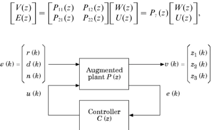
In modern control theory, all control structures can be described by using a generalized control framework, as depicted in Figure 1. The variables and functions in the Z domain are all capitalized. The framework contains a controller C(z) and an augmented plant P(z). The controlled variable v(k) corresponds to various control objectives z1(k), z2(k) and z3(k), and the extraneous input w(k) consists of the reference r(k), the distubance d(k),
and the noise n(k). The signals u(k) and e(k) are the control input to the plant and the measured output from the plant, respectively. The general input–output relation can be expressed as
$
V(z) E(z)%
=$
P11(z) P21(z) P12(z) P22(z)%$
W(z) U(z)%
= Pg(z)$
W(z) U(z)%
, (1)where the submatrices Pij(z), i, j = 1, 2 are compatible partitions of the augmented plant
Pg(z), and the signal variables are capitalized to represent the symbols in the Z domain.
The rationale of the Hacontrol is to minimize the infinity norm of the transfer function TVW(z) between v(k) and w(k), where the infinity norm represents the output energy (in
l2 norm) for the worst input of energy less than or equal to unity. It is straightforward
to show that Tvw(z) can be expressed as [10]
TVW(z) = P11(z) + P12(z)C(z) [1 − P22(z)C(z)]−1P21(z). (2)
Hence, the mathematical statement of the optimal Ha problem reads
min
C(z) >TVW(z)>a= minC(z) 0E u Q 2psup >TVW(e
ju)>. (3)
With the optimal Ha controller, best tracking performance, disturbance, rejection, and
uncertainty accommodation can be achieved under the condition that the whole system is internally stable. However, instead of the optimal solution that is generally very difficult to find, one is content with the suboptimal solution of the so-called standard Haproblem:
finding C(z) such that >TVW(z)>aQ 1.
2.2.
In this section, the feedback structure, the feedforward structure, and the hybrid structure are formulated on the basis of the aforementioned generalized control framework. In the feedforward and hybrid structure, it is further assumed that only the acoustical reference at the upstream of the canceling source is available, as usually is the case in practical applications. Because the upstream feedforward microphone will pick up both the noise from the primary source and the noise produced by the canceling loudspeaker, the positive acoustic feedback problem can no longer be ignored. It is this positive feedback problem that considerably complicates the active control design and so limits the performance and stability of the ANC system.
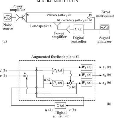
First, the feedback structure is illustrated in Figure 2. To find an Ha controller, one
weighs the error signal e(k) by W1(z), the control input u(k) by W2(z), and the plant output y(k) with W3(z). At this point, it is relevant to introduce two important sensitivity
functions: the sensitivity function S (z) and the complementary sensitivity function T (z) defined as [9]
S (z) = 1/[1 + P2(z)C(z)] (4)
and
T (z) = P2(z)C(z)/[1 + P2(z)C(z)]. (5)
The sensitivity functions S (z) and T (z) are, respectively, the indices of the system’s ability to cope with disturbances and uncertainties [9]. For good disturbance rejection, the normal performance condition must be satisfied
>S (z)W1(z)>aQ 1. (6)
On the other hand, to maintain stability of the system against plant perturbations and model uncertainties, the robustness condition that can be derived from the small-gain theorem must be satisfied [9]
>T (z)W3(z)>aQ 1. (7)
In general, W1(z) is chosen as a lowpass function and W3(z) is chosen as a highpass
Figure 2. Feedback ANC structure: (a) experimental setup; (b) block diagram.
band is more of a concern and plant uncertainties tend to fall in high frequencies due to, for example, modal truncation. It is yet very difficult to simultaneously minimize both sensitivity functions by simply noting that S (z) + T (z) = 1. The tradeoff between S (z) and
T (z) is further complicated by the waterbed effect. That is, one cannot minimize either
sensitivity function in a frequency range without inducing amplification of the same function at the other frequencies if the plant is at non-minimum phase [10]. This classical tradeoff between the performance and robustness renders the following mixed sensitivity problem [9]
>=S (z)W1(z)= + =T (z)W3(z)=>aQ 1. (8)
The input–output relation of the augmented plant corresponding to the feedback structure is
K
Z1(z)L
K
W1(z) −W1(z)P2(z)L
G
Z2(z)G
G
G K
L
= 0 W2(z) D(z) , (9)G
G
G
G
G
G
Z3(z) 0 W3(z)P2(z) U(z)G
G
G
G k
l
k
E(z)l
k
1 −P2(z)l
where P1(z) is the primary path and P2(z) is the secondary path. Hence, the suboptimal
condition of the feedback controller can be shown to be
N&
W1(z)S (z) W2(z)R(z) W3(z)T (z)'N
a
P3 (z) C (z) Power amplifier Noise source Loudspeaker Primary path P1 (z) Secondary path P2 (z) Power amplifier Digital controller Signal analyzer Error microphone d (k) u (k) e (k)
Augmented feedforward plant G + + (b) (a) path P3 (z) Acoustical feedback Upstream detector W1 (z) z1 (k) W2 (z) z2 (k) P1 (z) C (z) P2 (z) + +
where S (z) and T (z) are defined by equations (4) and (5), and R(z) = C(z)/[1 + P2(z)C(z)].
The additional weighting function W2(z) is used to limit the control input u(k) and is
generally chosen to be a small constant.
Next, consider the acoustic feedback problem. As has been mentioned previously, acoustic feedback generally causes detrimental effects to the ANC systems whenever feedforward sensors are used, such as the feedforward structure and the hybrid structure in our case. However, it will become clear later that acoustic feedback is naturally incorporated into the Ha synthesis procedure. Indeed, the merit of the Ha general
framework lies in the fact that it does not require special treatment insofar as acoustic feedback is concerned. The block diagram of the feedforward structure with acoustic feedback is illustrated in Figure 3. The input–output relation of the augmented plant corresponding to the feedforward structure is
&
Z1(z) Z2(z) E(z)'
=&
W1(z)P1(z) 0 1 W1(z)P2(z) W2(z) P3(z)'
$
D(z) U(z)%
, (11)where P3(z) is the transfer function of the acoustic feedback path. Dropping (z) for
convenience, the suboptimal condition of the Hafeedforward controller can be shown to
be
B$
W1FSW2FR
%B
aQ 1, (12)where
FS = P1(1 − CP3) + CP2/(1 − CP3), FR = C/(1 − CP3).
Figure 3. Feedforward ANC structure including an acoustical feedback path: (a) experimental setup; (b) block diagram. The shaded block indicates the acoustic feedback path.
C2 (z) Power amplifier Noise source Loudspeaker Primary path P1(z) Secondary path P2(z) Power amplifier Signal analyzer Error microphone u (k) e2 (k)
Augmented hybrid plant G
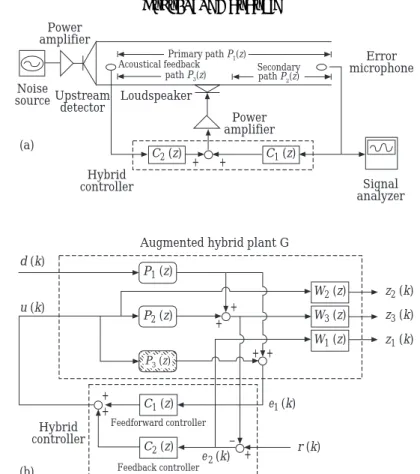
+ + (b) (a) path P3(z) Acoustical feedback Upstream detector W1 (z) z1 (k) W3 (z) z3 (k) P1 (z) C1 (z) + + C1 (z) + + P2 (z) W2 (z) z2 (k) C2 (z) e1 (k) r (k) + + Feedforward controller Hybrid controller Feedback controller – d (k) + P3 (z) Hybrid controller
Figure 4. Hybrid ANC structure including an acoustical feedback path: (a) experimental setup; (b) control block diagram. The shaded block indicates the acoustic feedback path.
FS(z) is the transfer function from the disturbance to the output. To achieve good
disturbance rejection, FS(z) should be small in the present low frequency control band. The downstream microphone output is weighed by W1(z) and the control input u(k) by W2(z). In general, W1(z) is chosen to be a lowpass function and W2(z) a small constant.
By the same token, the block diagram of the hybrid structure with acoustic feedback is illustrated in Figure 4. Dropping (z) for convenience, the input–output relation of the augmented plant corresponding to the hybrid structure is
Z1 W1 −W1P1 −W1P2
K L
K
L
G G
Z2G
0 0 W2G K L
RG G
Z3 =G
0 W3P1 W3P2G G G
D . (13)G G
G
G G G
E1 1 −P1 −P2 UG G
G
G k l
E2 0 1 P3k l
k
l
Hence, the suboptimal condition of the Ha hybrid controller can be shown to be
N&
W1HS W2HR W3HT −W1[P1(1 − C2P3) + C2P2]HS W2[C2(z) − C1(z)P1]HS W3[P1(1 − C2P3) + C2P2]HS'N
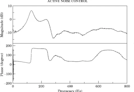
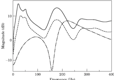
a Q 1, (14)Figure 5. The frequency response of the primary path plant. —, Measured curve; ---, modelled curve.
where
HS = (1 − C2P3)/(1 − C2P2+ C1P2), HR = (C2− P1C1)/(1 − C2P3+ C1P2),
and
HT = (P1(1 − C2P3) + C2P2)/(1 − C2P3+ C1P2).
HS(z) represents the transfer function from the disturbance to the downstream
microphone output. HT(z) is the transfer function associated with the unstructured
multiplicative uncertainty [10] for the hybrid structure. In the structure, one weighs the error
T 1 The models of the primary path , secondary path , and the acoustical feedback path of the duct identified by the ARX procedure Primary path Secondary path Acoustical feedback path delay = 5, gain = −0·0641 dealy = 1, gain = 0·9089 delay = 1, gain = 0·0064 ZXXXXXXXCXXXXXXXV ZXXXXXXXCXXXXXXXV ZXXXXXXXCXXXXXXXV zeros poles zeros poles zeros poles (−1·7519 −0·9446 −0·5625 2 0·6278i −0·8745 (−1·7519 −0·7250 (1·0369 2 0·0706i −0·8639 2 0·2333i −0·1412 2 0·8068i − 0·6287 2 0·5669i (−1·0706 −0·7521 2 0·4749i 0·5948 2 0·7568i −0·7408 2 0·4752i −0·3310 2 0·6297i −0·5297 2 0·6706i ( 1·0389 −0·8119 2 0·2015i 0·6995 2 0·3955i −0·5923 2 0·6439i 0·2763 2 0·8562i −0·3523 2 0·7715i 0·9233 −0·4763 2 0·7045i 0·3147 2 0·8005i −0·4231 2 0·7432i 0·6592 2 0·6741i −0·1286 2 0·8607i (2·0484 2 1·8137i −0·3262 2 0·7085i 0·1822 2 0·7931i −0·2251 2 0·8700i (1·0633 0·3184 2 0·8165i (1·0837 2 2·0421i −0·0983 2 0·8864i −0·2188 2 0·8650I 0·0814 2 0·8060i 0·4148 2 0·3587i 0·5475 2 0·6839i 0·6327 2 0·6693i 0·3223 2 0·8489i −0·5331 2 0·7142i 0·3095 2 0·8262i 0·8927 0·7766 2 0·4995i 0·5956 2 0·6923i 0·2237 2 0·7123i −0·7162 2 0·4606i 0·5782 2 0·7653i −0·4849 0·9629 2 0·1435i 0·3143 2 0·7870i 0·6590 2 0·6588i −0·7992 2 0·2037i 0·7640 2 0·4875i −0·2726 0·6336 2 0·3425i −0·8401 2 0·3254i 0·7800 2 0·4911i −0·7025 0·5964 2 0·4081i — −0·1661 −0·0532 2 0·7865i 0·8501 2 0·2237i — 0·9252 2 0·1603i — — −0·4994 2 0·4428i 0·9679 2 0·1476i — 0·9129 — — −0·2340 2 0·6325i — — 0·7411 — — — — ( Denotes non-minimal phase zeros
signal e2(k) by a low-pass W1(z), the control input u(k) by a small constant W2(z), and
the downstream microphone output by a high-pass W3(z).
Recognizing that plant uncertainties and perturbations will affect the performance of ANC systems, it is desirable to quantitatively assess the performance robustness of the forging three ANC structures. This is done by defining the following performance robustness (PR) index of how performance of disturbance rejection varies with respect to plant perturbations:
PR = lim
DP(z):0
DTyd(z)/Tyd(z)
DP(z)/P(z) =1ln (T1ln (P(z))yd(z))=
0
1TDP(z)yd(z)10
TP(z)yd(z)1
, (15)where the performance function Tyddenotes the transfer function from the disturbance d(k)
to the output y(k) and P(z) denotes the transfer function of the plant of interest. As can be seen in the definition, the larger the PR is, the worse the performance of disturbance rejection becomes in the presence of plant perturbations. In what follows, the PR indices
PR1, PR2, and PR3stand for the PR indices associated with the primary path P1(z), the
secondary path P2(z), and the acoustic feedback path P3(z), respectively, of the duct.
As will be seen shortly in the experimental results, a further improvement against plant perturbations can be achieved by the hybrid control structure. This interesting feature of hybrid control has also been noted by some other researchers [13, 14].
3. EXPERIMENTAL INVESTIGATIONS
Experiments were performed to compare the Ha-based ANC structures in the presence
of acoustic feedback problem. The Hacontroller synthesis technique is employed to design
an active electronic silencer for a duct. A rectangular duct of cross-section 0·25 × 0·25 m and length 1 m is used for the experiment, which renders the cutoff frequency 690 Hz. Within this control bandwidth, two fourth order Butterworth low-pass filters of cutoff frequency 600 Hz are employed as the antialiasing filter and reconstruction filter. The sampling rate is selected to be 2 kHz. The upstream reference microphone and error
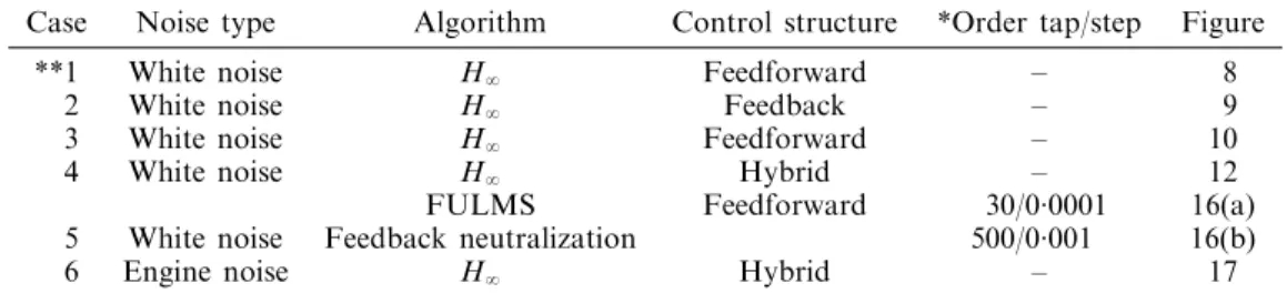
T 2
Experimental cases of the active electronic silencer for a duct
Case Noise type Algorithm Control structure *Order tap/step Figure
**1 White noise Ha Feedforward – 8
2 White noise Ha Feedback – 9
3 White noise Ha Feedforward – 10
4 White noise Ha Hybrid – 12
FULMS Feedforward 30/0·0001 16(a)
5 White noise Feedback neutralization 500/0·001 16(b)
6 Engine noise Ha Hybrid – 17
* Order, tap/step denotes either the order of the IIR filter for both the numerator and denominator, and the step size used in the FULMS algorithm, or the tap length of the FIR filter and the step size used in the feedback neutralization method.
** Case 1 is a reference case of purely feedforward control in the absence of acoustic feedback.
microphone are located at 0·25 m and 0·75 m, respectively, from the source end. It may first appear that the duct is very short compared to its cross-section, where the causality problem and excessive acoustic feedback may arise. This is indeed an unwilling compromise to make so that the the plant can be of sufficient low order below the cutoff frequency and numerical problems with the Ha calculation can be minimized. Besides,
causality is a simplified criterion applicable to infinite-length ducts only. For the finite-length duct at hand, the complex dynamics of the acoustic system are reflected by the poles and zeros, but not simply the pure time delays as in the case of infinite-length ducts. On the other hand, the duct is lined with some fiberglass sound-absorbing material to provide appropriate damping for the system. The importance of passive damping that has often been overlooked in active design lies in not only high frequency attenuation but also the robustness of active control with respect to plant uncertainties [15]. With sufficient damping treatment, the order of plant uncertainty is generally less than that of the unlined duct. On the other hand, the error microphone is placed in the close vicinity of the control loudspeaker to form the so-called collocated control. In doing so, the waterbed effect in conjunction with non-minimal phase zeros and time delay can be alleviated [9, 16].
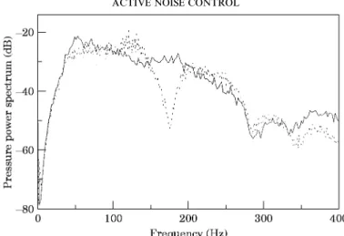
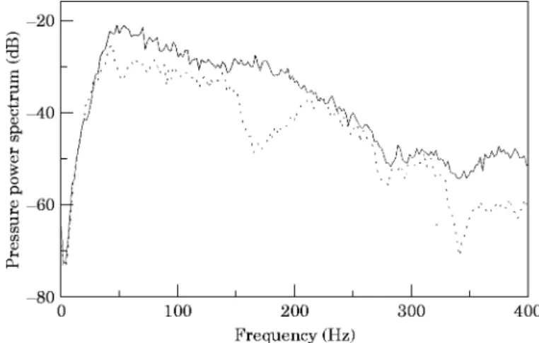
Figure 8. The residual sound pressure spectra of Case 1 for the white noise in the absence of acoustical feedback before and after ANC is activated by using the purely feedforward Hacontroller. —, Control off; ---, control
Figure 9. The residual sound pressure spectra of Case 2 for the white noise source when acoustical feedback is present before and after ANC is activated by using the Hafeedback controller. Key as for Figure 5.
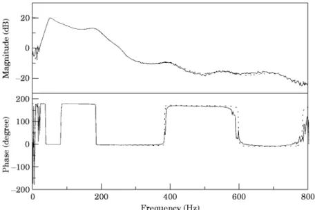
In the experiment, the mathematical models of the primary path, the secondary path and acoustical feedback path are established via an ARX system identification procedure [17]. The identified poles and zeros of these three plants are listed in Table 1. The frequency responses of the primary path, the secondary path, and the acoustical feedback path are shown in Figures 5–7, respectively. On the basis of the plant models, the Ha synthesis
procedure is applied to obtain the Hacontroller. The controller is then coded into a digital
filter on the platform of a floating-point DSP, TMS320C31. The experimental arrangements are illustrated in Figures 2(a), 3(a), and 4(a) for the feedback structure, the feedforward structure, and the hybrid structure, respectively. In addition, three synthetic as well as practical noise types, including a Gaussian white noise, an engine exhaust noise and an impact noise are chosen for comparing the different ANC structures. The experimental case design is shown in Table 2.
Case 1 is a reference case of purely feedforward Ha control, where the source voltage
signal is used as the feedforward reference so that acoustic feedback can be neglected. It
Figure 10. The residual sound pressure spectra of Case 3 for white noise source when acoustical feedback is present before and after ANC is activated by using the Hafeedforward controller. Key as for Figure 8.
T 3 The poles and zeros of the feedback controller delay = 0, gain = −0·1280 zeros (−2·9311 −0·8762 −0·9756 −0·7016 2 0·2218i −0·2417 2 0·8509i poles − 0·9801 −0·8531 −0·8023 −0·7190 −0·4830 2 0·6829i zeros −0·4763 2 0·7045i −0·3582 2 0·6160i −0·7250 −0·3262 2 0·7085i −0·0983 2 0·8864i poles −0·3866 2 0·7704i −0·3335 2 0·6933i −0·2206 2 0·7853i −0·1049 2 0·8777i −0·3871 2 0·1128i zeros 0·3223 2 0·8489i 0·4660 2 0·7756i 0·2237 2 0·7123i 0·0044 0·0928 poles 0·3196 2 0·8828i −0·0003 0·3170 2 0·7497i 0·2561 2 0·5695i 0·4275 2 0·7483i zeros 0·6283 2 0·7327i 0·5821 2 0·5469i 0·6590 2 0·6588i 0·4977 2 0·2561i 0·6335 poles 0·2953 2 0·3680i 0·6640 2 0·6908i 0·6361 2 0·6557i 0·4810 0·9754 2 0·1493i zeros 0·5192 0·8053 2 0·4126i 0·7562 2 0·5021i 0·9911 0·9272 poles 0·9818 2 0·0441i 0·9924 0·9351 0·8664 2 0·1298i 0·6888 2 0·5185i zeros 0·9603 2 0·1314i 0·9579 2 0·1476i 0·8501 2 0·2237i 0·7822 2 0·4891i 0·7800 2 0·4911i poles 0·8044 2 0·4186i 0·8350 2 0·4186i 0·7791 2 0·5313i 0·7788 2 0·4977i – ( Denotes non-minimal phase zeros. T 4 The poles and zeros of feedforward controller delay = 0, gain = 0·3725 zeros *−1·0125 −0·9756 −0·7367 2 0·3400i −0·5724 2 0·5447i −0·2417 2 0·8059i poles −0·2228 2 0·7830i −0·7419 2 0·2637i −0·5260 2 0·4643i −0·5420 2 0·3497i −0·5067 zeros −0·3582 2 0·6160i 0·1132 2 0·8661i 0·4660 2 0·7756i 0·5821 2 0·5469i 0·8998 2 0·4702i poles 0·2704 2 0·9413i 0·1332 2 0·8898i 0·3838 2 0·7692i −0·1020 0·6763 2 0·6445i zeros 0·7822 2 0·4891i 0·9603 2 0·1314i 0·9462 0·6335 −0·1020 poles 0·8539 2 0·5105i 0·9743 2 0·1807i 0·4790 0·9604 0·9621 ( Denotes non-minimal phase zeros
Figure 11. The predicted performance function Tyd(z) of three active noise controllers for the duct. —,
Feedforward controller; - - - - , feedforward controller in the presence of acoustical feedback; – · – · , hybrid controller in the presence of acoustical feedback.
can be seen from the result of Figure 8 that significant attenuation (approximately 5–20 dB) is obtained in the frequency range 40–200 Hz. In Cases 2–4, the signal detected by an upstream microphone is used as the feedforward reference so that the effect of acoustic feedback can no longer be ignored in the feedforward and the hybrid structures. In these cases, the HaANC systems are employed for attenuating the white noise. In the
experimental results shown in Figure 9, it can be observed that the noise attenuation reaches approximately 20 dB at 175 Hz, but the effective band appears quite narrow (145–180 Hz). The poles and zeros of the feedback controller are listed in Table 3. The total attenuation within the dominant band 0–400 Hz is found to be 2·02 dB. The experimental results of the Ha feedback control show similar waterbed effect to that of
the H2control [18] and the pole placement method [19], and in these cases only narrowband
attenuation can be achieved. It is found in the H2method that noise attenuation is obtained
in the band 200–320 Hz at the expense of creating peaks at higher frequencies. In the pole placement technique, the attenuation is observed at the first two modes (47 Hz and 95 Hz, respectively).
Figure 12. The residual sound pressure spectra of Case 4 for the white noise source when acoustical feedback is present before and after ANC is activated by using the Hahybrid controller. Key as for Figure 8.
T 5
The poles and zeros of hybrid controller
Feedforward part Feedback part
delay = 0, gain = 0·1108 delay = 0, gain = −0·1237
ZXXXXXXXXCXXXXXXXXV ZXXXXXXXXXCXXXXXXXXXV
zeros poles zeros poles
−0·9801 −0·9803 (−3·3641 −0·9803
−0·8536 −0·8398 − 0·8879 −0·8398
−0·9756 −0·8264 −0·9756 −0·8264
−0·7250 −0·7364 −0·7666 0·7364
−0·59562 0·6923i −0·59342 0·6922i −0·58362 0·7081i −0·59342 0·6922i −0·47632 0·7045i −0·48172 0·6807i −0·7250 −0·48172 0·6807i −0·44392 0·7825i −0·44822 0·7854i −0·44132 0·7938i −0·44822 0·7854i −0·09832 0·8864i −0·38502 0·7648i −0·30842 0·8506i −0·38502 0·7648i −0·32622 0·7085i −0·29982 0·8688i −0·47632 0·7045i −0·29982 0·8688i −0·39992 0·7295i −0·33162 0·6935i −0·15712 0·9104i −0·33162 0·6935i −0·29922 0·8666i −0·15202 0·9215i −0·35822 0·6160i −0·15202 0·9215i −0·35822 0·6160i −0·22142 0·7848i −0·24172 0·8059i −0·22142 0·7848i −0·14972 0·9207i −0·10102 0·8757i −0·32622 0·7085i −0·10102 0·8757i −0·24172 0·8059i 0·06812 0·9241i 0·06372 0·9400i 0·06812 0·9241i −0·1020 0·13362 0·8844i −0·09832 0·8864i −0·13362 0·8844i
0·07042 0·9221i −0·1694 0·11322 0·8661i −0·1694
0·11322 0·8661i 0·25152 0·8673i 0·27392 0·8749i 0·25152 0·8673i 0·32232 0·8489i 0·31802 0·8784i −0·0670 0·31802 0·8784i
0·22372 0·7123i 0·0001 0·32232 0·8489i 0·0001
0·26532 0·8560i 0·0331 0·50902 0·8052i 0·0331
0·50362 0·7872i 0·30622 0·7624i 0·46602 0·7756i 0·30622 0·7624i 0·46602 0·7756i 0·23162 0·5719i 0·22372 0·7123i 0·23162 0·5719i 0·41522 0·6802i 0·50482 0·7883i 0·29952 0·5814i 0·50482 0·7883i 0·65902 0·6588i 0·42882 0·7452i 0·62032 0·7336i 0·42882 0·7452i 0·95792 0·1476i 0·33592 0·5933i 0·58212 0·5469i 0·33592 0·5933i 0·85012 0·2237i 0·66362 0·6933i 0·65902 0·6588i 0·66362 0·6933i (1·0295 0·63622 0·6564i 0·84542 0·5052i 0·63622 0·6564i
0·9975 0·97022 0·1803i (1·1395 0·97022 0·1803i
( Denotes non-minimal phase zeros.
In contrast to the feedback structure, a broader band of attenuation can be obtained by using the feedforward structure. In Figure 10, significant attenuation up to approximately 12–22 dB of the random noise has been achieved throughout the band 150–220 Hz by using the feedforward control and total attenuation within the band 0–400 Hz is found to be 2·96 dB. The poles and zeros of feedforward controller are listed in Table 4.
In viewing the above results of noise attenuation, it is instructive to plot the transfer functions between the disturbance and the downstream microphone of the three ANC structures (Figure 11). The feedback structure displays only very narrowband noise rejection, as have been confirmed by the experimental results. The feedforward structure and the hybrid structure appear to have comparable performance, both better than that of the feedback control. Nevertheless, it is noteworthy that the experimental results reported in Figure 12 show considerable improvement of the hybrid structure over the feedforward structure. Attenuation has been achieved in two regions, 40–200 Hz and 330–400 Hz, by using the hybrid control and the poles and zeros of hybrid controller are listed in Table 5. Attenuation up to approximately 20 dB is obtained in the first region and 18 dB in the second region. The total attenuation within the band 0–400 Hz is found
Figure 13. The performance robustness index PR1of three active noise controllers for the duct in the presence
of acoustical feedback. —, Feedback controller; - - - - , feedforward controller; – · – · , hybrid controller.
to be 3·42 dB. This result is of comparable order with the theoretical prediction except some minor discrepancy due to modeling error by using the ARX procedure. Some additional insights can be obtained by calculating the PR indices, as shown in Figures 13–15. The indices PR1, PR2and PR3of the feedforward structure are the largest
among the ANC structures in most of the frequencies, while the indices PR1and PR2of
the feedback structure are the smallest. That is, the performance of the feedforward control is the most susceptible to plant uncertainties among the ANC structures, while the performance of the feedback control is the most robust against the plant perturbations. As a compromise between the feedforward control and the feedback control, the robustness of performance of the hybrid control is partially improved by the introduction of the feedback structure. Hence, the experimental results of the hybrid control agree more closely with the predicted performance than the feedforward control.
Figure 14. The performance robustness index PR2 of the three active noise controllers for the duct in the
Figure 15. The performance robustness index PR3of active noise feedforward and hybrid controller for the
duct in the presence of acoustical feedback. - - - - , Feedforward controller; —— , hybrid controller.
In the fifth case, two commonly used methods for dealing with acoustical feedback, the FULMS method and the feedback neutralization method, are employed in the present experiment for comparison with the proposed techniques. The details of these two methods can be found in reference [12] and are omitted here for brevity. Both the orders of the numerator and the denominator of the IIR filter used in FULMS method are 30. The tap length of FIR controller in the feedback neutralization technique is 300. The step size is 0·0001 in the two methods. The FULMS method produces 3–20 dB attenuation in the frequency range 50–200 Hz (Figure 16(a)). Total attenuation within the band 0–400 Hz is found to be 2·42 dB. The result was obtained 1 min after the active control was activated. However, a strong peak was found at 235 Hz in the spectrum of the FULMS algorithm. It appears that the FULMS method is prone to stability problems for the algorithm is trapped in a local minimum (because its performance index is generally not quadratic) and
Figure 16. The residual sound pressure spectra of Case 5 for the white noise source when acoustical feedback is present before and after ANC is activated: (a) FULMS method; (b) the feedback neutralization method. Key as for Figure 8.
Figure 17. The residual sound pressure spectra of Case 8 for the engine exhaust noise when acoustical feedback is present before and after ANC is activated by using the Hahybrid controller. Key as for Figure 8.
the control drifts away slowly so that the system can be unstable. As pointed out by the reviewer, the problem with stability may be solved by using the leaky LMS algorithm [12]. On the other hand, the experimental results of the feedback neutralization method are shown in Figure 16(b). Almost no attenuation can be obtained by using this method, the detrimental effect of acoustic feedback being evident from these results. Irrespective of which method used, the performance of noise attenuation is significantly degraded in comparison with the purely feedforward control in Case 1.
In the last case dealing with more practical noise, an exhaust noise from a 2000 cm3
gasoline engine running at 4000 r.p.m., is investigated by using the Hahybrid controller.
The results are shown in Figure 17. Signifiicant attenuation, approximately 20 dB and 12 dB can be observed at the second and third peak of the power spectra and total attenuation within the band 0–400 Hz is found to be 5·43 dB.
4. CONCLUSIONS
Three ANC structures of active noise cancellation for ducts: feedback control, feedforward control, and hybrid control have been compared in this paper by using a general framework of the Ha robust control theory. The Ha synthesis procedure
incorporates, without special treatment, the acoustic feedback path that is usually a plaguing problem to feedforward control design. Three ANC systems have been practically implemented by using a DSP.
The characteristics of each ANC structure, as indicated in the experimental results, can be summarized as follows. The main advantage of the feedback control is that no reference input is needed so that the acoustic feedback problem can be avoided. Nevertheless, the feedback control suffers from the waterbed effect due to time delay and non-minimum phase zeros and only narrowband noise rejection is achievable. For a high order plant such as a duct in our case, feedforward control appears to be a more viable approach for broadband noise rejection at the expense of performance robustness against plant uncertainties. Alternatively, hybrid control can be used to simultaneously achieve broadband noise rejection and robust performance. In comparison with the
feedforward control, the feedback control, and the well-known FULMS method, the experimental results of the Ha hybrid controller exhibit excellent performance for
suppressing stationary and transient noises, even in the presence of serious acoustic feedback. Nevertheless, it is remarked that the experimental duct is very short compared to its cross-section in the study, which might violate the causality constraint that is generally used as a design criterion of an infinite-length duct. The experimental results may be improved with a longer duct, provided the increased order of plant models is not an issue.
Despite the preliminary success, the Hahybrid controller is a fixed controller that may
not be able to accommodate excessive plant perturbations, e.g., large temperature variations in a muffler. It is reported in Eriksson’s work [20] that an adaptive controller with online plant modelling is capable of tracking such plant variations (despite some drawbacks detailed in the book by Kuo and Morgan [12]). From the same perspective, combination of the fixed and the adaptive controllers may make it possible to improve the robustness and thus will be explored in a future study.
ACKNOWLEDGMENTS
Special thanks go to Professors F. B. Yeh and M. C. Tsai for the helpful discussions on the Hacontrol theory. The work was supported by the National Science Council in
Taiwan, Republic of China, under the project number NSC 83-0401-E-009-024.
REFERENCES
1. S. J. E and P. A. N 1993 IEEE Signal Processing Magazine 10, 12–35. Active noise control.
2. C. R. F and A. H. F 1995 IEEE Control Systems Magazine 2, 9–19. Active control of sound and vibration.
3. J. C. B 1981 Journal of the Acoustical Society of America 70, 715–726. Active adaptive sound control in a duct: a computer simulation.
4. L. J. E 1990 Journal of the Acoustical Society of America 89, 257–265. Development of the filter-u algorithm for active noise control.
5. V. E and H. G. L 1982 Journal of the Acoustical Society of America 71, 608–611. Active attenuation of noise: the monopole system.
6. J. C. D, K. G, P. K, and B. A. F 1989 IEEE Transactions on Automatic Control 34, 832–847. State space solution to standard H2and Hacontrol problems. 7. P. A. I and K. G 1991 International Journal of Control 54, 1031–1073. State-space
approach to discrete-time Hacontrol.
8. I. Y and U. S 1991 IEEE Transactions on Automatic Control 36, 1264–1271. Transfer function approach to the problems on discrete-time systems: Ha optimal linear control and filtering.
9. J. C. D, B. A. F and A. R. T 1992 Feedback Control Theory. New York: Macmillan Publishing Company.
10. F. B. Y and C. D. Y 1992 Post Modern Control Theory And Design. New York: Eurasia. 11. M. C. T and C. S. T 1995 International Journal of Control 5, 155–173. A transfer matrix
framework approach to the synthesis of Ha controllers.
12. S. M. K and D. R. M 1996 Active Noise Control Systems Algorithms and DSP Implementations. New York: John Wiley.
13. M. M and E. Z 1989 Robust Process Control. Englewood Cliffs, N.J.: Prentice-Hall. 14. H. I and H. H 1995 Proceedings of International Symposium on Active Control of Sound and Vibration, ’95 875–880. Active noise control system based on the hybrid design of feedback and feedforward control.
15. R. G, A. H. F and D. W. V 1993 Journal of Guidance, Control and Dynamics 16, 662–667. Passive damping for robust feedback control of flexible structures.
16. G. F. F, J. D. P and A. E-N 1994 Feedback Control of Dynamic Systems. Reading, M.A.: Addison-Wesley.
17. L. L 1987 System Identification: Theory for the User. Englewood Cliffs, N.J.: Prentice-Hall. 18. J. H, J. C. A, R. V, M. N. L, A. G. S, P. D. W and D. S. B 1996 IEEE Transactions on Control Systems Technology 4, 283–291. Modeling, identification and feedback control noise in an acoustic duct.
19. A. J. H, C. R. R and S. C. S 1993 ASME Journal of Dynamic Systems, Measurement and Control 115, 488–494. Global active noise control of a one-dimensional acoustic duct using a feedback controller.
20. L. J. E and M. C. A 1989 Journal of the Acoustical Society of America 85, 797–802. Use of random noise for on-line transducer modeling in an adaptive active attenuation system.