新竹科學園區產業群聚因素影響分析

國

立

交

通

大

學

科技管理研究所

博 士 論 文

新竹科學園區產業群聚因素影響分析

Assessing the Critical Factors to Industrial

Clustering in Taiwan HsinChu Science Park

博 士 研 究 生：孫嘉祈

指導教授：林亭汝 博士

新竹科學園區產業群聚因素影響分析

Assessing the Critical Factors to Industrial

Clustering in Taiwan HsinChu Science Park

研 究 生：孫嘉祈 Student：Chia-Chi Sun

指導教授：林亭汝 博士 Advisor：Grace T R Lin

國 立 交 通 大 學

科技管理研究所

博 士 論 文

Dissertation

Submitted to Institute of Management of Technology College of Management

National Chiao Tung University in partial Fulfillment of the Requirements

for the Degree of Ph. D in

Management of Technology

June 2009

Hsinchu, Taiwan, Republic of China

新竹科學園區產業群聚因素影響分析

學生：孫 嘉 祈 指導教授：林 亭 汝 博士

國立交通大學科技管理研究所博士班

摘要

本論文將分為兩部分研究，首先，本論文將預測新竹科學園區半導體產業與電腦周 邊產業，2001 年至 2007 年之產值預測，本論文應用平滑指數模型、灰預測模型與馬可 夫灰預測模型為預測工具，由預測結果得知半導體產業其成長率呈現緩慢下降趨勢，而 電腦周邊產業則為衰退趨勢，半導體產業與電腦周邊產業其產值超過新竹科學園區整體 產值之百分之五十，而台灣產業群聚為台灣國家競爭優勢主要來源，產業群聚能提升生 產力，促進新企業發展與創新，並提升行銷與顧客關係，因此，如何改善新竹科學園區 整體產值下降，對於企業家與政府而言將是一個重要且急迫的任務，基於此，引發本論 文進行第二部分之研究， 本論文第二部分研究欲瞭解產業群聚發展背後之驅動力為何，本論文引用 Porter (1980) 國家競爭優勢與群聚驅動力概念，為本論文第二階段之探討主軸。 本論文試著探討不同驅動力對產業成長之影響程度，並探索驅動力彼此間之關係程 度， 基於此研究目的，本論文以鑽石模型 (Porter, 1980) 與文化概念，探討產業成長驅 動力之優先排序情況，本論文以DEMATEL 為研究工具，探討不同驅動力之影響關係， 並描繪出驅動力之因果關係圖，判別何者為影響驅動力，何者為被影響驅動力 以提供 台灣產業與政府相關策略建議，由研究結果得知主要影響驅動力為要素秉賦條件與當地 需求條件，而產業結構、策略與競爭程度，相關支援產業與政府支援為台灣新竹科學園 區群聚成長之間接驅動力 最後本論文將根據研究結論提出相關群聚政策，以幫助政府

或產業分析師改善台灣產業群聚政策。

Assessing the Critical Factors to Industrial

Clustering in Taiwan HsinChu Science Park

Student: Chia-Chi Sun Advisors: Dr. Grace T R Lin

Institute of Management of Technology

National Chiao Tung University

ABSTRACT

This research includes two parts. First, we want to forecast the annual output using the exponential smoothing forecasting model, the GM (1, 1) model, and the Grey-Markov model. The period of this research is from 2001 to 2007. The computer and semiconductor industries are the research examples for estimating model. From our estimation results, we understand that the annual output of the semiconductor industry will slow down in the future while that of the computer industry has a decreasing trend. The annual values of semiconductor industry and computer industry account for over 50% for the Hsinchu Science Industrial Park (HSIP). Industrial clusters can be seen as a main source of national competitiveness, serving to upgrade productivity, new business formation and innovation, and advance marketing/customer relations for Taiwan. Therefore, how to improve the alarmingly decreasing annual output and industrial value of HSIP is a critical and urgent task for industrial practitioners and government officials of Taiwan now and in the future. This point therefore triggers our research motivation for next step.

Therefore, the second part of this research is to contribute to the understanding of the casual and effect factors among those influencing an industrial cluster. Another core viewpoint anchored in this section is that national competitive advantages can be achieved by industrial clusters. That is, we would like to make use of the concepts of national competitiveness proposed by Porter (1980) and cluster drivers toward cluster value to conduct

our second part of research.

We try to examine the impacts of and determine the relationships among different driving forces. To this end, we adopt the Diamond Model (Porter, 1998) in addition to the concept of culture to give the priority to these driving forces. This research then applies the Decision Making Trial and Evaluation Laboratory (DEMATEL) to address the related issues. Discussing the relationship between different drivers and making a causal map that finds out the causal group and effect group, this research provides Taiwan industries and government with some strategic recommendations. From our results, we know that the major causal dimensions are local demand conditions and factor conditions. The factors of cure, firm structure, strategy, and rivalry, related and supporting industries, and government support as the indirect factors will be affected by the two causal factor, factor conditions and local demand conditions for the growth of industrial clusters in Taiwan. Finally we will attempt to draw upon our policy analysis results in order to assist government officials or industrial analysts in improving Taiwan’s industrial cluster policy and fostering the growth of the clusters.

Keywords:

Grey forecasting model, Markov chain, industrial cluster, driving force, Taiwan Hsinchu Science Park, Decision Making Trial and Evaluation Laboratory (DEMATEL)

誌 謝

三年前的六月，在驚訝中收到榜單，三年前的九月，帶著惶恐與喜悅的心情，來到 新竹，來到交通大學科管所，這一切一切感覺就像昨天才發生一樣。 回首當時，對環境感到恐懼，對同學感到陌生，對課業也不怎上手，其實滿辛苦， 就在慢慢適應之下，漸漸瞭解學校環境，也於所上認識許多同學，包括碩班、碩專班與 博班學長姐，彼此課業上互相幫助與討論，生活上互相分享心得，在此要特別感謝我的 指導教授 - 林亭汝老師，老師總是細心指導如何撰寫論文，林老師總是犧牲休息時間 與假日，與我討論論文，幫我修改論文，老師總是有耐心逐字看完我文章，再逐句與我 解釋，教導我研究方法與寫作技巧；另外，老師時時關心我生活情形和修課狀況，也教 導我許多人生道理，對老師滿懷感激與感恩，在此，跟老師說聲：老師，謝謝您。另外， 感謝虞孝成教授、袁建中教授、徐作聖教授、洪志洋教授於課業上教導，讓我對於科技 管理領域能有更深入瞭解，也奠定我未來研究基礎。 這次論文能順利完成，也要感謝這次口試委員徐作聖老師、虞孝成老師、劉世南老 師、吳信宏老師、吳宗修老師於口試時給我許多寶貴建議，使得論文其結構更為完整， 也使論文內容更為紮實。此外，同時也感謝幾位接受訪問與填答之專家，提供寶貴意見， 對本研究提供建設性建議，使論文更為豐富。 博士班生涯雖然辛苦，同學與學弟妹鼓勵與打氣，是我繼續前進動力，要感謝博班 同學友嵐、雅迪、啟陽、志杰、佳翰、蒧均、依錦、素雲，有你們的協助，讓我更順利 完成學業，也謝謝博班學弟妹崑銘、慶瑋、柔臻、豐光、邦寧、嘉麗、萬隆、永祺、佩 翰、榮新、光彬平時照顧，與同門學弟妹毓廷、運佳(The Rock)、亦泰、培芳關心打氣， 讓我博班生活更加多采多姿，也預祝你們學業順利。 最後，要感謝我爸媽和我哥，因為有您們的支持與鼓勵，讓我更有勇氣面對挑戰， 有您們無私奉獻，才能成就今日的我，我今日的成果，因為背後有您們最偉大的推手， 在此，將此喜悅與榮耀與您們分享。 孫嘉祈 謹誌於 國立交通大學科技管理研究所 中華民國九十八年六月

Table of Contents

摘要

... i

ABSTRACT ...iii

誌 謝 ... v

Table of Contents... vi

List of Tables ...viii

List of Figures ... ix

Chapter 1 Introduction ... 1

1.1

Research Background... 1

1.2

Research Motivation and Purpose ... 1

1.3

Dissertation Organization ... 5

Chapter 2 A Hybrid Grey Forecasting Model for Taiwan Clustering Growth

... 6

2.1

Background... 6

2.2

Taiwan’s Semiconductor and Computer Industries in Hsinchu

Science Park ... 10

2.3

The Exponential Smoothing Forecasting Model... 11

2.4

Grey Forecasting Model GM (1, 1)... 13

2.5

Markov Residual Modified Model ... 16

2.6

Error Analysis... 18

2.7

The Empirical Application Using the Samples of Hsinchu Science

Park 19

2.7.1

The Data of computer and semiconductor industries ... 19

2.7.2

The Research Framework of Estimation Annual Outputs 20

2.7.3

The Empirical Result of the Exponential Smoothing

Forecasting Model ... 21

2.7.4

The Empirical Result for the Grey Model... 23

2.7.6

Error Measurement and Analysis ... 29

2.8

Summary... 32

Chapter 3 Driving Industrial Clusters to be Nationally Competitive... 34

3.1

Background... 34

3.2

What Factors Drive Industrial Clusters to be nationally

Competitive? ... 37

3.2.1

Factor Conditions ... 38

3.2.2

Local Demand Conditions... 39

3.2.3

Related and Supporting Industries ... 39

3.2.4

Firm Structure, Strategy, and Rivalry ... 40

3.2.5

Government Support... 40

3.2.6

Culture ... 41

3.2.7

Cluster Drivers and System-effects... 41

3.3

The Decision Making Trial and Evaluation Laboratory

(DEMATEL) Method ... 43

3.4

Empirical Evidence from Hsinchu Science Park ... 46

3.4.1

Research Framework of Measuring the Driving Forces ... 47

3.4.2

Identify Relationship between Driving Forces Using

DEMATEL ... 47

3.4.3

Discussions... 52

3.5

Conclusion... 59

Chapter 4 Dissertation Conclusions and Suggestions... 62

References ... 67

Appendix I WEF Ranking of the Competitiveness of Industrial Clusters .. 76

Appendix II The profile of ten experts ... 77

List of Tables

Table 1Output value of the Computer and Semiconductor Industries in

Hsinchu Science Industrial Park from 2001 to 2007 (in NT$ billion)... 20

Table 2 Actual Output Value, Historical Forecasted Output Value, and

Residual Error of the Exponential Smoothing Model for the Computer

Industry (in NT$ billions) ... 22

Table 3 Actual Output Value, Historical Forecasted Output Value, and

Residual Error of the Exponential Smoothing Model for the Semiconductor

Industry (in NT$ billions) ... 23

Table 4 Actual Output Value, Historical Forecasted Output Value, and

Residual Error of Grey Model for the Semiconductor Industry (in NT$

billions) ... 25

Table 5 Actual Output Value, Historical Forecasted Output Value, and

Residual Error of Grey Model for the Computer Industry (in NT$ billions)

... 26

Table 6 Actual Output Value, Historical Forecasted Output Value, and

Residual Error of Markov Modified Model for the Semiconductor Industry

(in NT$ billions) ... 28

Table 7 Actual Output Value, Historical Forecasted Output Value, and

Residual Error of Markov Modified Model for the Computer Industry (in

NT$ billions)... 29

Table 8 Dimensions of the Driving Forces for the Growth of Industrial

Clusters... 49

Table 9 Direct-Influence Matrix ... 50

Table 10 Direct-Relation Matrix ... 50

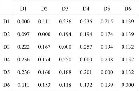
Table 11 Total-Influence Matrix... 51

List of Figures

Figure 1 Framework of estimation the annual outputs ... 20

Figure 2 Trend of the actual value and historical forecast value for the

semiconductor industry ... 31

Figure 3 Trend of the actual value and historical forecast value for the

computer industry ... 31

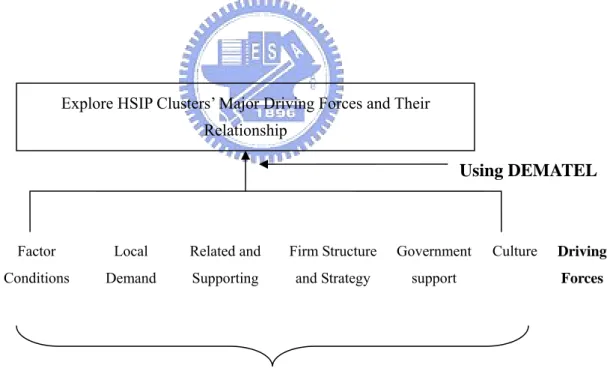
Figure 4 Research Framework of measuring the driving forces for HSIP.. 47

Figure 5 Impact-Relationship Map ... 52

Chapter 1 Introduction

1.1 Research Background

Taiwan owns the world’s largest manufacturing companies of high-tech components and products. According to the World Economic Forum’s “2007-2008

Global Competitiveness Report,” Taiwan has again taken first place in the world in the “State of Cluster Development” index. HsinChu Science Industrial Pak (HSIP)

was established in northwestern Taiwan as a focal point for high-tech R&D and production. Since the park’s beginnings, in 1980, the government has invested

approximately US$3.67 billion in it. By the end of March 2007, 475 high-tech companies in six industries (integrated circuits, computers and peripherals,

telecommunications, optoelectronics, precision machinery, and biotechnology) were situated within the 625-hectare park. At the end of 2006, the park’s total paid-in

capital exceeded US$35.4 billion, and more than 100 park companies were listed on Taiwan's main exchange, the Taiwan Stock Exchange, and on over-the-counter

markets (Chen, 2007)

1.2 Research Motivation and Purpose

Industrial clusters can be characterized as being networks of production of

strongly interdependent firms (including specialized suppliers), knowledge producing agents (universities, research institutes, engineering companies), bridging institutions

(brokers, consultants) and customers, linked to each other in a value adding production chain. It is clear that clusters are dependent upon informal contacts which

are based upon trust and reciprocity. Equally the transfer of ideas and a common labor pool enhances competition and reinforces the competitive advantage of the cluster as

development, and the local organizations and institutions that evolved to serve them (Cortright and Mayer, 2001). Ketels (2003) argued that clusters develop over time;

they are not a phenomenon that just appears or disappears overnight. Clusters develop because regional proximity among firms promotes learning and competence building.

The industrial cluster will attract similar and related firms because they want to exploit the common knowledge base and take part in the interactive learning that

takes place.

Cluster development, however, should be derived from cluster growth. Economic

growth can primarily be explained and measured by per capita income output (Marshall, 1920; Rostow, 1960; Hicks, 1946; Lewis, 1955). Likewise, usually the

growth of industrial cluster can be evaluated by annual industrial output changes. There are some examples to measure the growth of industrial clusters in

literature. Sull (2001) adopted an embedded case study design that explores the growth of the U.S. automotive tire industry at the level of the industry as a whole, the

cluster centered in Akron, Ohio and constituent firms. Sull (2001) takes a historical perspective, covering the period between the emergences of the automotive tire

industry in the early 1900s through to 1988, by which time only a single major U.S. tire manufacturer remained after all others had been acquired by European or

Japanese competitors. Moore (1978) proposed a method of characterizing the growth using two parameters, a production index measuring growth, and a structural change

index measuring the change in the composition of output. Liu (2004) examined the sources of structural changes in output growth of China’s industrial cluster over

1987–1992 using a decomposition method.

As noted above, the HSIP will be our dissertation topic. Most specifically, this

research applied historically quantitative forecasting methods to measure the growth of industrial clusters by observing and analyzing the changes of related industrial

output at HSIP. They are exponential smoothing forecasting model, the GM (1, 1) model, and the Grey-Markov model. We want to forecast the annual output using the

exponential smoothing forecasting model, the GM (1, 1) model, and the Grey-Markov model. The period of this research is from 2001 to 2007. The computer and

semiconductor industries are the research examples for estimating model. The first part of this research is to understand and estimate the annual output growth trend.

However in this section we offered an extra contribution which relates to offering an example as to how people in the future can apply a good estimation tool for industrial

output efficiency. From the research results, the error rates for the exponential smoothing model are 13.48% and 13.49% for the two industries. The relative

percentage errors of the GM (1, 1) model are 6.7116% and 7.20% for our surveyed industries. Notably, after the GM (1, 1) was modified using the Markov chain, the

semiconductor industry’s annual output of absolute error decreased to 6.54%, while the computer industry’s annual output of absolute error decreased to 7.01%. Thus, our

research results indicate that Grey-Markov estimating model is much more accurate for estimating the annual output of the semiconductor and computer industries in the

case of HSIP.

From our estimation results, we also understand that the annual output of the

semiconductor industry will slow down in the future while that of the computer industry has a decreasing trend. The annual values of semiconductor industry and

computer industry account for over 50% for the HSIP. Industrial clusters can be seen as a main source of national competitiveness, serving to upgrade productivity, new

business formation and innovation, and advance marketing/customer relations for Taiwan. Therefore, how to improve the alarmingly decreasing annual output and

our research motivation for next step.

Therefore, the second part of this research is to contribute to the understanding of

the casual and effect factors among those influencing an industrial cluster. Another core viewpoint anchored in this section is that national competitive advantages can be

achieved by industrial clusters. That is, we would like to make use of the concepts of national competitiveness proposed by Porter (1980) and cluster drivers toward cluster

value to conduct our second part of research.

We try to examine the impacts of and determine the relationships among different

driving forces. Hence, we attempt to find out the impact of the major driving forces behind HSIP clustering and to measure the relationships among those forces. These

factors of industrial clusters also exist for improving national competitiveness. To this end, we adopt the Diamond Model (Porter, 1998) in addition to the concept of culture

to give the priority to these driving forces. Based on deductions from the prior literature, the driving forces in question are factor conditions, local demand conditions,

related and supporting industries, firm structure and strategy and rivalry, government support, and culture. This research then applies the Decision Making Trial and

Evaluation Laboratory (DEMATEL) to address the related issues. Discussing the relationship between different drivers and making a causal map that finds out the

causal group and effect group, this research provides Taiwan industries and government with some strategic recommendations. It is because we believe that

Taiwan can be viewed as an appropriate case demonstrating how her industrial clustering have resulted in particular national competitiveness, and from this

perspective we wish to find out how those drivers associate with each other, finally leading to successful forms of clusters. Moreover, we attempt to draw upon our policy

analysis results in order to assist government officials or industrial analysts in improving Taiwan’s industrial cluster policy and fostering the growth of the clusters.

1.3 Dissertation Organization

The dissertation is organized as follows. Section 2 is the first part. It presents a hybrid grey forecasting model for Hsinchu Science Industrial Park. Section 3 is the

second part. It applies the DEMATEL method to find out the impact of the major driving forces behind HSIP clustering and to measure the relationships among those

Chapter 2 A Hybrid Grey Forecasting Model for Taiwan Clustering

Growth

2.1 Background

Cluster development, however, should be derived from cluster growth. Economic growth can primarily be explained and measured by per capita income output

(Marshall, 1920; Rostow, 1960; Hicks, 1946; Lewis, 1955). Likewise, usually the growth of industrial cluster can be evaluated by annual industrial output changes. This

research applied historical quantitative forecasting methods to measure the growth of industrial clusters.

The historical forecasting of annual output in high-tech industries is useful for companies to prepare marketing strategies and perform production capacity planning

and for financial institutions to make investment decisions (Chang, Lai, and Yu, 2003). This work attempts to forecast the annual output of semiconductor and

computer industries of Hsinchu Science Industrial Park (HSIP) historically. HSIP provides a unique environment for accelerating technological innovation, nurturing

new start-up firms, attracting investment, and generating economic growth (Potworowski, 2002). According to the historical forecasting analysis, industrial

practitioners can understand market trends and customer’s needs and, in turn, modify their production strategies and replan their resources and capacities.

Taiwan is one of the world’s largest manufacturers of high-tech components and products. According to the World Economic Forum’s “2007-2008 Global

Competitiveness Report,” Taiwan has again taken first place in the world in the “State of Cluster Development” index (see Appendix 1). HSIP was established in

northwestern Taiwan as a focal point for high-tech R&D and production. Since the park’s beginnings, in 1980, the government has invested approximately US$3.67

billion in it. By the end of March 2007, 475 high-tech companies in six industries (integrated circuits, computers and peripherals, telecommunications, optoelectronics,

precision machinery, and biotechnology) were situated within the 625-hectare park. At the end of 2006, the park’s total paid-in capital exceeded US$35.4 billion, and

more than 100 park companies were listed on Taiwan's main exchange, the Taiwan Stock Exchange, and on over-the-counter markets (Chen, 2007).

We can look to past research studies to observe the many historical forecasting methods that have been employed over the years, including quantitative and

qualitative methods. Qualitative forecasting methods include the expert system and the Delphi method. Quantitative forecasting methods then include regression analysis,

exponential smoothing, neural networks, and the Grey forecasting model (Chang et al., 2003).

Of the various forecasting models, the exponential smoothing model has been found to be one of the most effective. Since Brown (1959) began to use simple

exponential smoothing to predict inventory demand, exponential smoothing models have been widely used in business and finance (Gardner, 1985). However,

exponential smoothing methods are only a class of linear model, and, thus, it can only capture linear features of financial time series. Furthermore, as the smoothing

constant decreases exponentially, the disadvantage of the exponential smoothing model is that it gives simplistic results that only use several previous values to

forecast the future. The exponential smoothing model is, therefore, unable to find subtle nonlinear patterns in the financial time series data.

The Grey forecasting model has numerous applications. Hsu and Chen (2003) examines the precision of the Grey forecasting model applied to samples based on

of Taiwan’s opto-electronics industry from 2000 to 2005. Chang (2004) uses a grey forecasting model GM (1, 1) to improve the estimation of systematic risk of the

classical capital asset pricing model.

In order to improve forecast accuracy, many researchers have modified the GM

(1, 1) model. Liang, Zhao, Chang, and Liang (2001) utilized an improved grey model GM (1, 1) combined with a statistical method developed to evaluate the durability of

concrete bridges due to carbonation damage. Yao, Chi, and Chen (2003) presented an improved Grey-based prediction algorithm to forecast a very short-term electric

power demand for the demand-control of electricity. Chang, Lai, and Yu (2005) constructed a rolling Grey forecasting model (RGM) to predict Taiwan’s annual

semiconductor production. Tien’s (2005) grey dynamic model DGDM (1, 1, 1) was first combined with the Grey-Markov chain forecasting model to predict the time for

which the deviation is over the limit of tolerance deviation. Lin and Lee (2007) proposed a novel forecasting model termed MFGMn (1, 1) and modified the

algorithm of the grey forecasting model to enhance the tendency catching ability. Wang (2004) provided empirical evidence using grey theory and fuzzy time series,

which do not require a large sample and long past time series. Yao et al. (2003) then presented an improved Grey-based prediction algorithm to forecast a very short-term

electric power demand for the demand-control of electricity.

In the current research, we mainly apply quantitative historically forecasting

methods to predict the annual output of computer and semiconductor industries in HSIP. First, we use an exponential smoothing method to historical forecast the annual

output. Then, we apply the historically grey forecasting model to predict in the same regard. This research has also adopted a novel high-precision historical forecasting

model, the Grey-Markov model, to enhance the prediction accuracy. Finally, we compare the prophecy accurateness among these three historical forecasting methods.

Again, we applied these historically quantitative forecasting methods to try to measure the growth of industrial clusters by observing and analyzing the changes of

2.2 Taiwan’s Semiconductor and Computer Industries in Hsinchu Science Park

Taiwan has created its computer and semiconductor industry cluster in HSIP. An

essential aspect of the cluster is its development of close cooperative relationships. More specifically, Taiwan has promoted its own “Silicon Valley” cluster located in

HSIP, which is organized and run by a government agency. The HSIP is virtually composed of all the Taiwan semiconductor firms engaged in every facet of the

business, from IC design to chip fabrication, testing and assembly, and the utilization of chips in system products such as computers, hubs, switches, and scanners.

The electronics industry is the largest and fastest growing manufacturing industry in the world. The rapid rate of globalization is made possible by the rapid

development and expansion of the Internet economy, which, in turn, is fueled by the unprecedented growth of high-tech electronics manufacturing. HSIP is one of the

world's most significant areas for semiconductor manufacturing. Taiwan semiconductor industry consists of more than 100 design companies, 20 firms

producing wafers, over 40 packaging firms, and 30 testing firms. Taiwan Semiconductor Manufacturing (TSMC) and United Microelectronics (UMC) have

become the number 1 and 2 IC foundry operators in the world, respectively (Chang et al., 2005).

Taiwan’s computer industries also play a dominant role around the world. Taiwan’s computer industries in HSIP become the largest in the world – this growth

has been accompanied by a transition from original equipment manufacture and original design manufacture to original design logistics (Wang, Chiu, and Chen, 2003).

The market share has ranked first globally from 2001 to 2007 (Sun and Lin, 2007; Hung, 2000).

2.3 The Exponential Smoothing Forecasting Model

The exponential smoothing methods are relatively simple approaches to

forecasting. Three basic variations of exponential smoothing are commonly used: simple exponential smoothing (Brown, 1959; Billah, King, Snyder and Koehler,

2006), trend-corrected exponential smoothing (Holt, 1957), and the Holt–Winters’ method (Winters, 1960).

The current research applies an exponential smoothing method that forecasts the annual output of the semiconductor industry and the computer industry in HSIP.

Suppose that the time series x x₁, ,₂ … is described by the following model: xn

0

t t

x =β ε+ ………..………(1)

where B is the average of the time series and ₀ ε_t is the random error. Then the

estimate x of _t β₀ made in time is given by the smoothing equation below. t 1

(1 )

t _{t t}

x =αx + −α x₋ ………(2)

where α denotes a weighted index, 0< < , If the value of α 1 α is equal to 1 (one) then the previous observations are ignored entirely; if it is equal to 0 (zero),

then the current observation is ignored entirely, and the smoothed value consists entirely of the previous smoothed value. Lai et al. (2006) applied the ordinary least square (OLS) to determine the value ofα. This research adopt Holt-independent model using a large parameter value (α=0.9) for smoothing the level component. Then

the value of x is the observation value of period t , and t x is the forecasting value t

of period . t

Thus, a point forecast made in time for t xt+1 is

1 (1 )

t _t t

x+ =αx + −α x ………(3)

1 (1 )

t _t t

x+ = + −x α x ………...………(4)

The Grey forecasting model and GM-Markov forecasting model are explained as following sections.

2.4 Grey Forecasting Model GM (1, 1)

Grey theory is one of the new mathematical theories born out of the concept of

the grey set (Chang and Kung, 2006). It is an effective method used to solve uncertainty problems with discrete data and incomplete information. The GM (1, 1) is

one of the most frequently used grey forecasting models. This model is a time series forecasting model, encompassing a group of differential equations adapted for

parameter variance rather than a first-order differential equation. Its difference equations have structures that vary with time rather than being general difference

equations (Chang, 2003). Although it is not necessary to employ all the data from the original series to construct the GM (1, 1), the potency of the series must be greater

than four. In addition, the data must be taken at equal intervals and in consecutive order without bypassing any data (Deng, 1986). The grey forecasting model has three

basic operations: (1) accumulated generation, (2) inverse accumulated generation, and (3) grey modeling (Mao and Chirwa, 2006). The mathematics concept is borrowed

from Mao and Chirwa (2006). The GM (1, 1) model construction process is described below.

Step 1: For an initial time sequence

( )

{

( )

_{( )}

( )

_{( )}

( )

_{( )}

( )

_{( )}

}

n x i x x x X 0 = 0 1, 0 2,…, 0 ,…, 0 ………(5)

Step 2: On the basis of initial sequence ( )0

X , a new sequence X( )1 is set up through

the accumulated generating operation in order to provide the middle message

of building a model and to weaken the variation tendency.

( )

{

_x( )

_{( )}

_x( )

_{( )}

_x( )

_{( )}

_{i x}( )

_{( )}

_n

}

X 1 = 1 1, 1 2,…, 1 ,…, 1 ………..(6)

( )

_{( )}

_{k x}( )

_{( )}

_{i k n} X k i , , 2 , 1 1 0 1 ₌

∑

_{= …} =

Step 3: The first-order differential equation of GM (1, 1) model is then the following:

( ) ( ) _b aX dt dX = + 1 1 ………(7)

and its difference equation is

( )

_{( )}

_{k aZ}( )

_{( )}

_{k b k n}

X 0 + 1 = =2,3,…,

and, from Equation (7), we get

( )

_{( )}

( )

_{( )}

( )

_{( )}

( )

_{( )}

( )

_{( )}

( )

_{( )}

⎥ ⎦ ⎤ ⎢ ⎣ ⎡ × ⎥ ⎥ ⎥ ⎥ ⎥ ⎦ ⎤ ⎢ ⎢ ⎢ ⎢ ⎢ ⎣ ⎡ − − − = ⎥ ⎥ ⎥ ⎥ ⎥ ⎦ ⎤ ⎢ ⎢ ⎢ ⎢ ⎢ ⎣ ⎡ b a n Z Z Z n x x x 1 1 3 1 2 3 2 1 1 1 0 0 0 ……….(8)

where and are the coefficients to be identified. Let a b

( )

_{( )}

( )

_{( )}

( )

_{( )}

[

T n x x x n Y = 0 2, 0 3,…, 0

]

……….(9) ( )

_{( )}

( )

_{( )}

( )

_{( )}

_⎥⎥ ⎥ ⎥ ⎥ ⎦ ⎤ ⎢ ⎢ ⎢ ⎢ ⎢ ⎣ ⎡ − − − = 1 1 3 1 2 1 1 1 n Z Z Z B ………..…………..……(10) also take ( )

₍

₎

(

( )

_{( )}

( )

₍

₁

₎

)

_{1,2, ,}

₍

₁ 2 1 1 1 1 1 _{+ = + + = −} n k k x k x k Z …

)

………..(11) and

[ ]

T b a A= , ………..(12)

where Ynand B are the constant vector and the accumulated matrix, respectively. ( )1

(

₊1 is the k Z

)

(

k+1

)

thbackground value.

( )

n T T Y B B B A= −1 ………..………(13)

Step 4: Substituting A in Equation (12) with Equation (13), the approximate

equation becomes the following:

( )

( )

( )

_{( )}

1 0 ( 1) 0 1 (1 ) 2,3, , , a a k b x k x e e a k n ∧ − − ⎛ ⎞ =_⎜ − _⎟ − ⎝ ⎠ = … … ………...……….(14)

where is the predicted value of at time

( )

(

1 1 + ∧ k x

)

(

+1

)

∧ k x

(

k+1

)

. After the

completion of an inverse-accumulated generating operation on Equation (15),

at time becomes available and, therefore,

( )

(

1 0 + ∧ k x

)

(

k+1

)

( )

(

k

)

x( )

(

k

)

x( )

( )

k x 1 1 0 1 1 ∧ ∧ ∧ − + = + ……….……….(15)

2.5 Markov Residual Modified Model

In order to improve on the GM (1, 1) model, we used the Markov chain to

modify the residual errors of GM (1, 1). We borrowed the mathematics concept from Hsu and Wen (1998) and Wang (2004).

Step 1: Define the residual series (0).

q (0) (0) (0) (0) (0) (0) (0) 0 (2), (3), , ( ) ( ) ( ) ( ), 2,3, , q q q q n where q k x k x k k n ⎡ ⎤ = ⎣ ⎦ = − = … … ………..……….(16)

Step 2: Denote the absolute values of the residual series as_{ε .} (0)

(0) (0) (0) (0) (0) (0) (2), (3), , ( ) ( ) ( ) , 2,3, , n where k q k k n ε ε ε ε ε ⎡ ⎤ = ⎣ = = … … ⎦ _{……….………..(17)}

Step 3: A GM (1, 1) model of _{ε can be established as follows:} (0) ( 1) (0) ( ) (1) b (1 a ) a k k e a ε ε ε ε ε ₌⎡ε ₋ ⎤ ₋ − − ⎢ ⎥ ⎣ ⎦ e ………..(18)

where ,a b_{ε ε} is estimated using OLS.

Step 4: Assume that the sign of the data residual is in state 1 when it is

positive and in state 2 when it is negative. A one-step transition probability is associated with each possible transition from state to state

kth P i j , and can be estimated using P / ij ij i

P =M M ,i=1, 2 and j=1, 2. M means the number of the years _i

whose residuals are statei, and M_ij is the number of transitions from state to

state

i

j that have occurred. These values can be presented as a transition

matrix

ij P

R.

Step 5: These P values can be arranged as a transition matrix:

11 12 21 22 P P R P P ⎡ = ⎢ ⎣ ⎦ ⎤ ⎥ ……….……….(19) where R can be estimated by examining the signs of residuals for all years.

Step 6: Denote the initial state distribution by the vector: (0) (0) (0) 1 , 2 π _{= ⎣}⎡π π ⎤_⎦, where π₁ is state 1(+) probabilities, and π₂ is state 2(-) probabilities. The state probabilities after ' transitions are given by

n π( )n π(0)Rn ′ ′ _{= , where} ( ) ( ) ( ) ( ) 1 , 2 n n n n π ′ _=⎡π ′ π ′ _⎤×π

⎣ ⎦ ′ are (n+n th′) year residual state probabilities. Let the sign

of the (n+n th′) year residual be represented as follows: ( ) (0) 1 2 ( ) (0) 1 2 1 ( ) , 1, 2, 1 n n if n n n if π π σ π π ′ ′ ⎧+ > ⎫ ⎪ ⎪ ′ + =_{⎨ ⎬} = − < ⎪ ⎪ ⎩ ⎭ ……….(20)

Step 7: An improved grey model with residual modification and Markov chain sign estimation can be formulated as follows:

(0) (0) _{(0) ( 1)} 0 (0) ₍₀₎ ( ) ( ) ( ) (1) (1 ) (1) (1), ( ) 1 a a k r r b x k x k k e e a where x x k ε ε ε ε σ ε σ − − ⎡ ⎤ = + _⎢ − _⎥ − ⎣ ⎦ = = ± ……….……..…….(21)

2.6 Error Analysis

To examine the accuracy of the different forecasting models, we compare the

historically forecasting results of the value using our samples from 2001 to 2007. Relative percentage error (RPE) compares the real and historical forecast values. The

equation for RPE can be formulated as follows:

( ) ( ) 100% ( ) x k x k RPE x k − = × ………..……….(22)

2.7 The Empirical Application Using the Samples of Hsinchu Science Park

The data of this work were obtained from the bureau of HSIP (see Table 1). The

period of this research is from 2001 to 2007. We want to historically forecast the annual output using the exponential smoothing forecasting model, the GM (1, 1)

model, and the Grey-Markov model. An evaluation of the performance and accuracy of the forecast model using the error evaluation technique is discussed. These

following sections will show the detailed stages.

2.7.1 The Data of computer and semiconductor industries

The samples of this research are two high-tech industries in HSIP, which are the computer and semiconductor industries. Please see the Table 1 below for details.

Table 1Output value of the Computer and Semiconductor Industries in Hsinchu Science Industrial Park from 2001 to 2007 (in NT$ billion)

Year Computer Industry Semiconductor Industry

2001 1610.71 3757.19 2002 1245.28 4562.59 2003 1347.71 5632.75 2004 1382.45 7427.38 2005 1018.8 6851.10 2006 1014.96 7947.94 2007 949.46 8192.14

Source: Bureau of Hsinchu Science Industrial Park, 2008

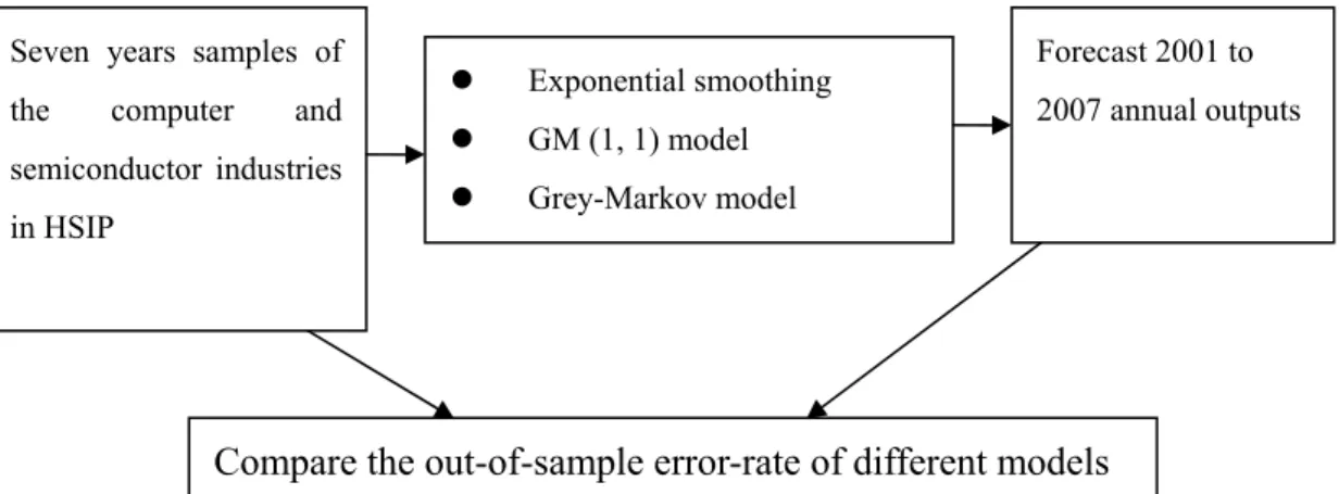
2.7.2 The Research Framework of Estimation Annual Outputs

The aim of this research is to historically forecast the annual output of the computer and semiconductor industries in Taiwan and examine the accuracy of

different historical forecasting methods. Thus, we identify which is the best among the exponential smoothing model, the GM (1, 1) model, and the Grey-Markov model.

Figure 1 illustrates the framework of this research.

Seven years samples of the computer and semiconductor industries in HSIP Forecast 2001 to 2007 annual outputs z Exponential smoothing z GM (1, 1) model z Grey-Markov model

Compare the out-of-sample error-rate of different models

2.7.3 The Empirical Result of the Exponential Smoothing Forecasting Model

The function of exponential smoothing is expressed byxt+1= +xt α(x_t−xt),

where α denotes a weighted index, 0< <α 1, x is the observation value of period _t , and

t x is the forecasting value of period . t t

The exponential smoothing prediction function for the computer industry is as follows, and the historical forecasting values are presented in Table 2.

1 ( ) 0

t t _t t

x+ = +x α x −x whereα = .9

In Table 2, the actual value, the historical forecasted output value, the residual error, and the average error are shown for the computer industry. Table 2 reveals that

Table 2 Actual Output Value, Historical Forecasted Output Value, and Residual Error of the Exponential Smoothing Model for the Computer Industry (in NT$ billions)

Year Actual Output

Value Historical Forecasted Output Value Residual Error (%) 2001 1610.71 2002 1245.28 1572.059 26.24% 2003 1347.71 1277.958 5.18% 2004 1382.45 1340.735 3.02% 2005 1018.8 1378.278 35.28% 2006 1014.96 1054.748 3.92% Computer industry 2007 949.46 1018.939 7.32% Average residual error 13.49%

The exponential smoothing prediction function for the semiconductor industry is

as follows, and the historical forecasting values are presented in Table 3.

1 ( ) 0

t t _t t

x+ = +x α x −x whereα = .9

In Table 3, the actual value, the historical forecasted output value, the residual

error, and the average error are shown for the semiconductor industry. Table 3 reveals that the residual error is 13.48%.

Table 3 Actual Output Value, Historical Forecasted Output Value, and Residual Error of the Exponential Smoothing Model for the Semiconductor Industry (in NT$

billions)

Year Actual Output

Value Historical Forecasted Output Value Residual Error (%) 2001 3757.19 3757.19 2002 4562.59 4015.344 11.99% 2003 5632.75 4507.865 19.97% 2004 7427.38 5520.262 25.68% 2005 6851.10 7236.668 5.63% 2006 7947.94 6889.657 13.32% Semiconductor industry 2007 8192.14 7842.112 4.27% Average residual error 13.48%

2.7.4 The Empirical Result for the Grey Model

The grey model GM (1, 1) is a time series prediction model (Wang, 2006). Based on GM (1, 1), the Grey historical forecasting model, and the data in Table 1, we

estimate the output value of the two industries from 2001 to 2007. The calculating steps are explained below.

Step 1: The original total annual sales series for the semiconductor industry is the following:

(0) _{{3757.19, 4562.59,5632.75,7427.38,6851.10,7947.94,8192.14}}

X =

Step 2: On the basis of the initial sequence ( )0

X , a new sequence X( )1 is set up. (1) _{[3757.19,8319.78,13952.53,21379.91,28231.01,36178.95,44371.09]}

X =

Step 3: The first-order differential equation of the GM (1, 1) model is then the following:

[

4562.59,5632.75,7427.38,6851.10,7947.94,8192.14

]

T n Y = -6038.485 1 -11136.155 1 -17666.22 1 -24805.46 1 -32204.98 1 -40275.02 1 B ⎡ ⎤ ⎢ ⎥ ⎢ ⎥ ⎢ ⎥ = ⎢ ⎥ ⎢ ⎥ ⎢ ⎥ ⎢ ⎥ ⎣ ⎦

( )

1

[

]

-0.0990706963, 4587.3422453666 T T n A= B B − B Y = Step 4

The forecast equation for the GM (1, 1) is as given below.

(0) _{0.0990706963 ( 0.0990706963)(k-1)} 0 ( ) 3757.19 4587.3422453666 (1 ) (-0.0990706963) 2,3, , 1, x k e e k n n − − − ⎛ ⎞ =_⎜ − _⎟× − × ⎝ ⎠ = … + …

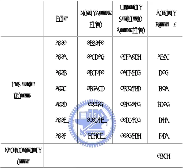
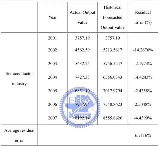
In Table 4, the actual value, the historical forecasted output value, the residual

error, and the average error are shown for the semiconductor industry. Table 4 also indicates that the residual error is 6.71%.

Table 4 Actual Output Value, Historical Forecasted Output Value, and Residual Error of Grey Model for the Semiconductor Industry (in NT$ billions)

Year Actual Output

Value Historical Forecasted Output Value Residual Error (%) 2001 3757.19 3757.19 2002 4562.59 5213.5617 -14.2676% 2003 5632.75 5756.5247 -2.1974% 2004 7427.38 6356.0343 14.4243% 2005 6851.10 7017.9794 -2.4358% 2006 7947.94 7748.8623 2.5048% Semiconductor industry 2007 8192.14 8555.8626 -4.4399% Average residual error 6.7116%

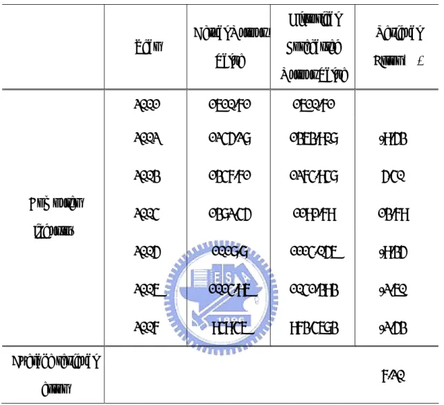
Similarly, in Table 5, the actual value, the historical forecasted output value, the residual error, and the average error are shown for the computer industry. Table 5 also

Table 5 Actual Output Value, Historical Forecasted Output Value, and Residual Error of Grey Model for the Computer Industry (in NT$ billions)

Year Actual Output

Value Historical Forecasted Output Value Residual Error (%) 2001 1610.71 1610.71 2002 1245.28 1363.908 -9.53% 2003 1347.71 1274.948 5.40% 2004 1382.45 1191.79 13.79% 2005 1018.8 1114.056 -9.35% 2006 1014.96 1041.393 -2.60% Computer industry 2007 949.46 973.4683 -2.53% Average residual error 7.20%

2.7.5 The Empirical Result for the Markov Modified Model

This research then applies a Grey-Markov chain model. The procedure of

estimation is basically the same as that for the grey model.

Step 1: Define the residual series (0).

q

[

]

(0) _{-650.9717,-132.7747,1017.3457,-166.8794,199.0777,-363.7226}

Step 2: Denote the absolute values of the residual series as_{ε .} (0)

[

]

(0) _{650.9717,132.7747,1017.3457,166.8794,199.0777,363.7226} ε = Step 3:

[

]

(1) _{650.9717,783.7464,1801.0921,1967.9715,2167.0492,2530.7718} ε = -717.3590 1 -1292.4192 1 -1884.5318 1 -2067.5104 1 -2348.9105 1 B ⎡ ⎤ ⎢ ⎥ ⎢ ⎥ ⎢ ⎥ = ⎢ ⎥ ⎢ ⎥ ⎢ ⎥ ⎣ ⎦

[

0.0781352204,505.8321788262

]

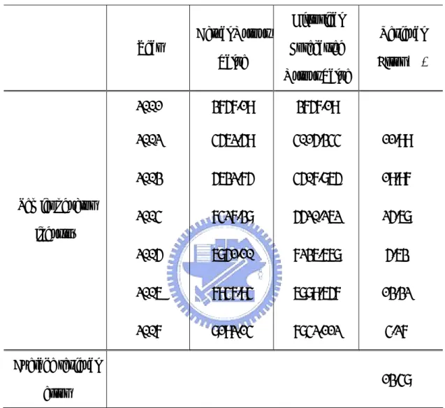
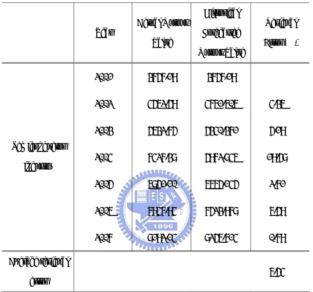
A= (0) _{0.0990706963 ( 0.0990706963)(k-1)} 0 0.0781352204) ( 0.0781352204)(k-1) 4587.3422453666 ( ) 3757.19 (1 ) (-0.0990706963) 505.8321788262 ( ) 0 (1 ) (-0.0781352204) 2,3, , 1, x k e e k e e k n n δ − − − − − − ⎛ ⎞ =_⎜ − _⎟× − × ⎝ ⎠ ⎡ ⎤ + _⎢ − _⎥× − ⎣ ⎦ = … + …

In Table 6, the actual value, the historical forecasted output value, the residual error, and the average error are shown for the semiconductor industry. Table 6 also

Table 6 Actual Output Value, Historical Forecasted Output Value, and Residual Error of Markov Modified Model for the Semiconductor Industry (in NT$ billions)

Year Actual Output

Value Historical Forecasted Output Value Residual Error (%) 2001 3757.19 3757.19 2002 4562.59 4761.606 4.36% 2003 5632.75 5340.371 5.19% 2004 7427.38 5972.846 19.58% 2005 6851.10 6665.145 2.71% 2006 7947.94 7523.978 6.59% Semiconductor industry 2007 8192.14 8256.714 0.79% Average residual error 6.54%

Furthermore, in Table 7, the actual value, the historical forecasted output value,

the residual error, and the average error are shown for the computer industry. Table 7 also indicates that the residual error is 7.01%.

Table 7 Actual Output Value,Historical Forecasted Output Value, and Residual Error of Markov Modified Model for the Computer Industry (in NT$ billions)

Year Actual Output

Value Historical Forecasted Output Value Residual Error (%) 2001 3757.19 3757.19 2002 4562.59 1228.203 1.37% 2003 5632.75 1167.335 13.38% 2004 7427.38 1106.455 19.96% 2005 6851.10 1046.386 2.71% 2006 7947.94 987.7313 2.68% Computer industry 2007 8192.14 930.9156 1.95% Average residual error 7.01%

2.7.6 Error Measurement and Analysis

Tables 2-7 list the residual errors of three historical forecast models using the RPE method. We adopted Equation (22) to measure the RPE among the three

historical forecasting models and obtained the arithmetic mean value for each model. The exponential smoothing method uses historical time series data to construct the

historical forecasting model. The error rates for the exponential smoothing model are 13.48% and 13.49% for the two industries in question. Recently, in order to improve

and scholars have applied the grey forecasting model. The comparison reveals that the GM (1, 1) model is more accurate than the exponential smoothing model. The RPE

for the GM (1, 1) model are 6.7116% and 7.20% for the semiconductor and computer industries respectively. Notably, after the GM (1, 1) was modified using the Markov

chain, the semiconductor industry’s annual output of absolute error decreased to 6.54% from 6.7116%, while the computer industry’s annual output of absolute error

decreased to 7.01% from 7.20%. Therefore, the Grey-Markov forecasting model is viewed as the most efficient tool among the three models for estimating the annual

output of the semiconductor and computer industries in the HSIP.

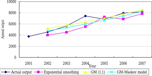
Figures 2-3 illustrate the actual value, the forecast from the exponential

smoothing model, the GM (1, 1) model, and the Grey-Markov model for the computer and semiconductor industries, respectively. These figures also show the trends of

annual output from 2001 to 2007. From the prediction, we understand that the annual output of the semiconductor industry will slow down in the future while that of the

computer industry has a decreasing trend. This implies a need for the industrial practitioners and the Taiwanese government to plan the industry’s direction and

strategies. In the meantime, they should reconsider the allocation of the research and development (R&D) resources and capacities.

Based on our research results, the annual output of semiconductor industry slow down in the future. Industrial practitioners for the semiconductor industry should

understand the market’s needs, providing unique and high-quality products and applying customer relationship management to continuously strengthen customer

satisfaction and loyalty. On the other hand, the computer industry has a decreasing trend. Industrial practitioners for this industry should consider how to upgrade

industrial competitive advantages. They need to acquire new technology and the necessary commensurate skill upgrades in order to improve their performance.

0 2000 4000 6000 8000 10000 2001 2002 2003 2004 2005 2006 2007 Year A nnua l outpu t

Actual output Exponential smoothing GM (1,1) GM-Maekov model

Figure 2 Trend of the actual value and historical forecast value for the semiconductor industry 0 500 1000 1500 2000 2001 2002 2003 2004 2005 2006 2007 Year Annual Outpu t

Actual output Exponential smoothing GM (1,1) GM-Maekov model

Figure 3 Trend of the actual value and historical forecast value for the computer industry

2.8 Summary

The current research presents an investigation of the annual output of the

semiconductor and computer industries in HSIP. The time period of this research is from 2001 to 2007. We wanted to forecast the annual output through the exponential

smoothing forecast model, the GM (1, 1) model, and the Grey-Markov model.

From the research results, the error rates for the exponential smoothing model are

13.48% and 13.49% for the two industries. The relative percentage errors of the GM (1, 1) model are 6.7116% and 7.20% for our surveyed industries. Notably, after the

GM (1, 1) was modified using the Markov chain, the semiconductor industry’s annual output of absolute error decreased to 6.54%, while the computer industry’s annual

output of absolute error decreased to 7.01%. Thus, our research results indicate that Grey-Markov estimating model is much more accurate for estimating the annual

output of the semiconductor and computer industries in the case of HSIP.

From our estimation results, we also understand that the annual output of the

semiconductor industry will slow down in the future while that of the computer industry has a decreasing trend. The annual values of semiconductor industry and

computer industry account for over 50% for the HSIP. Industrial clusters can be seen as a main source of national competitiveness, serving to upgrade productivity, new

business formation and innovation, and advance marketing/customer relations for Taiwan. Therefore, how to improve the alarmingly decreasing annual output and

industrial value of HSIP is a critical and urgent task for industrial practitioners and government officials of Taiwan now and in the future. This point therefore triggers

our research motivation for next step.

Therefore, the second part of this research is to contribute to the understanding of

the casual and effect factors among those influencing an industrial cluster. Another core viewpoint anchored in second section is that national competitive advantages can

be achieved by industrial clusters. That is, we would like to make use of the concepts of national competitiveness proposed by Porter (1998) and cluster drivers toward

cluster value to conduct our second part of research.

We try to examine the impacts of and determine the relationships among

different driving forces. Hence, we attempt to find out the impact of the major driving forces behind HSIP clustering and to measure the relationships among those forces.

These factors of industrial clusters also exist for improving national competitiveness. To this end, we adopt the Diamond Model (Porter, 1998) in addition to the concept of

culture to give the priority to these driving forces. Based on deductions from the prior literature, the driving forces in question are factor conditions, local demand conditions,

related and supporting industries, firm structure and strategy and rivalry, government support, and culture. This research then applies the Decision Making Trial and

Evaluation Laboratory (DEMATEL) to address the related issues. Discussing the relationship between different drivers and making a causal map that finds out the

causal group and effect group, this research provides Taiwan industries and government with some strategic recommendations. It is because we believe that

Taiwan can be viewed as an appropriate case demonstrating how her industrial clustering have resulted in particular national competitiveness, and from this

perspective we wish to find out how those drivers associate with each other, finally leading to successful forms of clusters. Moreover, we attempt to draw upon our policy

analysis results in order to assist government officials or industrial analysts in improving Taiwan’s industrial cluster policy and fostering the growth of the clusters.

Chapter 3 Driving Industrial Clusters to be Nationally Competitive

3.1 Background

The increasing competition and globalization of industries, markets, and technologies has raised the demand for outside-in innovation and acquisition of

technology through integrated innovation clusters (Becker and Gassmann, 2006). Companies need to develop cluster competence in order to link their organizations to

other players in the market to allow interactions beyond organizational boundaries (Ritter and Gemunden, 2004).The formation of clusters of innovation is a useful

concept for transforming both tangible and intangible knowledge into embodied and disembodied technical change (Liyanage, 1995; Isbasoiu, 2006).

Clusters are defined as selected sets of multiple autonomous organizations, which interact directly or indirectly, based on one or more agreements between them (Carroll

and Reid, 2004; Lin, Tung and Huang, 2006). The aim of clusters is to gain a competitive advantage for the individual organizations involved and occasionally for

the entire cluster as well. Cluster competence enables a company to establish and use relationships with other organizations (Ritter and Gemunden, 2004; Mills, Reynolds

and Reamer, 2008).

Previous studies also have examined the cluster structure (Ritter and Gemunden,

2004; Gemunden, Ritter, and Heydebreck, 1996; Clark and Guy, 1998), and some studies have addressed the cluster effect (Teng, Tseng, and Chiang, 2006). A number

of empirical studies have also provided evidence that clusters affect innovation performance (Colombo and Delmastro, 2002). Particularly, in past studies scholars in

the field of innovation systems have found it most useful to compare innovation systems between different industries or countries (Chang and Shih, 2004).

Some scholars have drawn attention to the Taiwanese innovation system (Hu, Lin, and Chang, 2005; Lee and Tunzelmann, 2005; Lai and Shyu, 2005; Tasi and Wang,

2005). Taiwan is one of the world’s largest manufacturers of high-technology components and products. According to the World Economic Forum’s “2007-2008

Global Competitiveness Report,” Taiwan has again taken first place in the world in the “State of Cluster Development” index (see Appendix 1) (Chen, 2007). The HSIP

is now one of the world's most significant areas for semiconductor manufacturing. It is home to the world's top two semiconductor foundries, Taiwan Semiconductor

Manufacturing Company (TSMC) and United Microelectronics Corporation (UMC) (Tasi and Wang, 2005; Lai and Shyu, 2005; Chen, 2007). The HSIP, established by the

government of Taiwan in 1980, straddles Hsinchu City and Hsinchu County on the island of Taiwan. Industries in the HSIP cover primarily six spheres—semiconductors,

computer peripherals, communications, opto-electronics, biotechnology, and precision machinery. Firms in the science park bring in high-tech industries and, in addition,

help transform Taiwan’s labor-intensive industries into technology-intensive industries.

On the other hand, while a number of studies have documented the significant role of innovation system as well as its possible cluster drivers, little is so far known

about the reflection of a link between national competitiveness and industrial cluster drivers. That said, related researches are mostly concerned with the topics of

innovation and cluster development. Drivers of industrial clusters are seldom explored from the perspective of national competitive advantages as a whole. For instance, Lai,

Chiu and Leu (2005) explored the effects of industrial cluster on innovation capacity, and to study the impact of external resources on firms’ innovation capacity especially

Knowledge Spillovers, Entrepreneurship, Path Dependence and Lock-In, Culture and Local Demand.

Accordingly, in next section we will then particularly introduce Porter’s diamond model targeting the issue of measuring as well as analyzing industrial clustering

linked to national competitiveness enhancement.

The DEMATEL is a suitable method that helps us in gathering group knowledge

for forming a structural model, as well as in visualizing the causal relationship of subsystems through a causal diagram (Wu and Lee, 2007). The other thing is that its

diagraphs are more useful than directionless graphs because diagraphs can demonstrate the directed relationships of sub-systems. Moreover, the diagraph

portrays a basic concept of contextual relation among the elements of the system, in which the numeral represents the strength of influence (Wu, 2008).

We take the HSIP for pursuing our case purposes. Discussing the relationship between different drivers and making a causal map that finds out the causal group and

effect group, this research provides Taiwan industries and government with some strategic recommendations. It is because we believe that Taiwan can be viewed as an

appropriate case demonstrating how her industrial clustering have resulted in particular national competitiveness, and from this perspective we wish to find out how

3.2 What Factors Drive Industrial Clusters to be nationally Competitive?

Kao, Wu, Hsieh, Wang, Lin and Chen (2008) applied four dimensions to measure the national competitiveness, such as economy, technology, human resource, and

management. Önse, Ülengin, Ulusoy, Aktaş, Kabak and Topcu (2008) adopted basic requirements factor, efficiency enhancers factor and innovation and sophistication

factor to estimate the national competitiveness. Wang, Chien and Kao (2007) examined the influence of technology development on national competitiveness. They

thought that technology development plays a key role in national competitiveness. Cho, Moon and Kim (2008) used eight variables to evaluate the national

competitiveness that include factor conditions, business context, related and supporting industries, demand conditions, human factors, politicians and bureaucrats,

entrepreneurs, professionals.

We believe that most of the above chiefly issue from a major breakthrough for

the cluster concept derived from Porter’s Competitive Advantage of Nations (1998), which advocated specialization according to historical strength by emphasizing the

power of industrial clusters. Porter highlighted that multiple factors beyond those internal to the firm may improve its performance. In his “diamond model,” four sets

of interrelated forces are brought forward to explain industrial clusters: factor input conditions; local demand conditions; related and supported industries; and firm

structure, strategy, and rivalry.

The industrial clusters stimulate innovation and improve productivity; they are a

critical element of national competitiveness (Cortright, 2002; Cooke, 2001; Porter, 1998). The core viewpoint anchored in this research is that national competitive

other approaches, the diamond model is therefore deemed our most fitting analytic framework while we are pursuing effective measurement of industrial cluster drivers

from the viewpoint of national competitive advantages. Our research also attempts to provoke discussion on the value of looking at the cultural influences on the growth of

clusters. This approach could be used to help determine the catalytic role that such development organizations should be playing by emphasizing the need to base

decision-making on cultural as well as on economic factors in order to stimulate cluster formation and enable innovation by optimizing cultural interchange.

The below describes key dimensions of national competitiveness, mainly derived from the Porter’s Diamond Model. And following the above arguments, these

dimensions can be also regarded as drivers of industrial clustering.

3.2.1 Factor Conditions

Porter agreed that a state’s or nation’s endowment of factors for encouraging

production has a role in determining competitive advantage. However, Porter broadened the definition of factors for production into five major categories: human

resources, physical resources, knowledge resources, capital resources, and infrastructure (Rojas, 2007).

Abundant natural resources, which are factors of production, could provide the original momentum for establishing an industry (Castells and Hall, 1994). Their

presence might also have enticed a predecessor industry to the location, thereby creating the initial framework for a subsequent industry (Porter, 1998).

The fact that competitive pressure compels firms to innovate in order to overcome their microeconomic environment’s disadvantages represents a major theme

in Porter’s work. The remaining fundamental determinants in the model play an important and powerful role in inciting firms to innovate so as to remain competitive

players in their industries. Specialized factors of production are skilled labor, capital, and information infrastructure. Specialized factors involve heavy, sustained

investment, and they are more difficult to duplicate. These factors include entrepreneurship and venture capital.

3.2.2 Local Demand Conditions

Consumer demand plays possibly the most important role in forming and building up an industrial cluster. A large number of industrial customers in the nearby

area create sufficient demand to enable suppliers to acquire and operate expensive specialized machinery.

Porter (1998) has argued that a sophisticated domestic market is an important element for producing competitiveness. Firms that face a sophisticated domestic

market are likely to sell superior products because the market demands high quality, and a close proximity to such consumers enables the firm to better understand the

needs and desires of the customers (Lai and Shyu, 2005). As a result, demand conditions can stimulate an industry through local demand for a product that also

proves viable in regional, national, and international markets (Woodward, 2004).

3.2.3 Related and Supporting Industries

Spatial proximity of upstream or downstream industries facilitates the exchange

of information and promotes a continuous exchange of ideas and innovations. The availability, density, and interconnectedness of vertically and horizontally related

industries are important drivers for industrial clusters (Lai and Shyu, 2005). This includes suppliers and related industries.