國 立 交 通 大 學
電 信 工 程 學 系 碩 士 班
碩 士 論 文
應用於 LZW 壓縮序列之高效能字串比對機制
Efficient Pattern Matching Scheme in LZW
Compressed Sequences
研究生 :黃迺倫
指導教授:李程輝 教授
Efficient Pattern Matching Scheme in LZW
Compressed Sequences
研 究 生: 黃迺倫
Student: Nai-Lun Huang
指導教授: 李程輝 教授
Advisor: Prof. Tsern-Huei Lee
國 立 交 通 大 學
電 信 工 程 學 系 碩 士 班
碩 士 論 文
A Thesis
Submitted to Department of Communication Engineering College of Electrical and Computer Engineering
National Chiao Tung University in Partial Fulfillment of the Requirements
for the Degree of Master of Science
in
Communication Engineering June 2006
Hsinchu, Taiwan, Republic of China.
應用於 LZW 壓縮序列之高效能字串比對機制
學生: 黃迺倫 指導教授: 李程輝 教授
國立交通大學電信工程學系碩士班
中文摘要
壓縮字串比對(CPM; compressed pattern matching)乃一新興之研究領域,著 眼於此類問題:給定一壓縮序列及一字串,在最少量之解壓縮作用(或無解壓縮 作用)下,於序列中尋找字串的出現(pattern occurrences)。可應用於直接在壓縮 檔案中做電腦病毒及機密資訊外洩漏與否的偵查。LZW 為一廣受應用且壓縮效 率高的壓縮演算法,本論文即記述了我們在壓縮字串比對上,對於處理 LZW 壓 縮序列的研究成果。著名的 Amir-Benson-Farach 演算法是最早能在 LZW 壓縮序 列中尋得字串的首次出現位置的演算法,我們針對此演算法提出一以位元串映像 為基礎的(bitmap-based)實現方式,同時亦將其推廣為可尋得所有的字串出現,並 回報它們在序列未壓縮前所處的絕對位置。程式模擬結果顯示,相較於解壓縮後 再於解開之序列中搜尋的機制,我們採用的機制具有較高的時間效能;而相較於 另一套同樣以位元串映像實現的壓縮字串比對演算法──Navarro-Raffinot 機 制,我們的機制對於中等長度以上的字串,在所需的記憶體空間上,是較為節省 的。 i
Compressed Sequences
Student: Nai-Lun Huang Advisor: Prof. Tsern-Huei Lee
Institute of Communication Engineering
National Chiao Tung University
Abstract
Compressed pattern matching (CPM) is an emerging research field addressing the problem: Given a compressed sequence and a pattern, find the pattern occurrence(s) in the (uncompressed) sequence with minimal (or no) decompression. It can be applied to detection of computer virus and confidential information leakage in compressed files directly. In this thesis, we report our work of CPM in LZW compressed sequences. LZW is one of the most effective compression algorithms used extensively. We propose a simple bitmap-based realization of the well-known Amir-Benson-Farach algorithm. We also generalize the algorithm to find all pattern occurrences (rather than just the first one) and to report their absolute positions in the uncompressed sequence. Experiments are conducted to compare the performance of our proposed generalization with the decompress-then-search scheme. We found that our proposed generalization is much faster than the decompress-then-search scheme. The memory space requirement of our proposed generalization is compared with that of the Navarro-Raffinot scheme, an alternative CPM algorithm which can also be realized with bitmaps. Results show that our proposed generalization has better space performance than the Navarro-Raffinot scheme for moderate and long patterns.
誌謝
由衷感謝我的指導教授──李程輝教授。在研究的過程中,您給予充分的信 任,讓我有足夠的空間思考,並選擇感興趣的題目著手研究。在您的教誨下,我 學到做研究的正確態度與方法,此外,您適時的鼓勵也讓我增加自信心。尤其感 謝您的悉心指導以及在本論文研究上所提供的各項建議與協助,讓我有機會將研 究成果投稿至IEE期刊,這對我來說是莫大的鼓舞。 感謝網路技術實驗室的魏震榮學長、郭耀文學長和謝景融學長在課業及研 究上的指教,也要感謝一起奮鬥的同窗夥伴──郁文、政家和紹瑜,不論在課業、 研究或生活上,都能不吝分享、相互勉勵,能成為你們之中的一份子,我感到幸 運而且珍惜。 最後,我要特別感謝我的父親黃金宗先生與母親柯祝女女士,感謝您們的 栽培與教養,以及無限的關懷和鼓勵,每當遭遇挫折,是您們給予我溫暖的避風 港,也是您們再度教會我勇敢,讓我能重拾信心,接受挑戰。同時,感謝我的男 友羅木榮先生所給予我的一切支持與包容。 謹將此論文獻給我的父親與母親。 西元2006年6月 於風城交大 iiiContents
中文摘要 i English Abstract ii 誌謝 iii Contents iv List of Tables v List of Figures vi Chapter 1 Introduction 1 Chapter 2 Background 4
2.1 The LZW Compression Algorithm 4
2.2 The Amir-Benson-Farach Algorithm 5
Chapter 3 An Efficient Pattern Matching Scheme in LZW
Compressed Sequences 11
3.1 An Efficient Realization of Amir-Benson-Farach Algorithm 11
3.2 Generalization to All Pattern Occurrences 16
Chapter 4 Related Work 24
Chapter 5 Comparison and Experimental Results 28
Chapter 6 Conclusion 34
List of Tables
List of Tables
Table 3-1. Prefix bitmaps of P = abcab 15
Table 3-2. Suffix bitmaps of P = abcab 15
Table 3-3. Prefix bitmaps of P = ababc 16
Table 3-4. Bitmaps associated with explicit nodes 16
Table 3-5. Prefix bitmaps of P = ababc 22
Table 3-6. Suffix bitmaps P = ababc 22
Table 3-7. Contents of nodes along the path from root to Np on Ts 22
Table 3-8. Brief summary of the results when the last three chunks are
processed 23
List of Figures
Figure 3-1. The uncompacted suffix trie STp of P = ababc 16
Figure 5-1. Performance comparison for test case 1 29
Figure 5-2. Performance comparison for test case 2 29
Figure 5-3. Comparison of space requirements for test case 3 32
Figure 5-4. Comparison of space requirements for test case 4 32
Figure 5-5. Comparison of space requirements for test case 5 33
Figure 5-6. Comparison of space requirements for different number of
Chapter 1 Introduction
Chapter 1
Introduction
As the population of communication networks users grows at a rapid rate, it is expected that the networks be capable of delivering data more effectively. In other words, how to utilize the transmission bandwidth efficiently is a key upon which the success of the communication networks heavily relies. Obviously, an economic way to utilize limited bandwidth efficiently is to send smaller amount of data by using data compression mechanisms. Accordingly, compressed pattern matching (CPM) that performs pattern search directly on the compressed data without initial decompression gains more and more attention. The CPM problem is often defined as: Given a compressed sequence and a pattern, find the pattern occurrence(s) in the (uncompressed) sequence with minimal (or no) decompression. Possible applications of CPM include detection of computer virus and confidential information leakage in compressed files directly.
Since LZW [1] is one of the most effective and popular lossless compression algorithms, CPM in LZW compressed sequences is quite important. In the last decade, many related researches have been conducted. The first CPM algorithm which finds the first pattern occurrence in an LZW compressed file was presented in [2]. The complexity of the algorithm is O(n+ ) in both time and space, where n and m are, respectively, the lengths of the compressed text and the pattern. It was shown that, with different implementations, one can trade between the amount of extra space used and the algorithmm’s time complexity. This algorithm is now
2
m
well-known and will be referred to as the Amir-Benson-Farach (ABF) algorithm in this thesis. Details of the ABF algorithm are presented in Chapter 2.2. In [3], the ABF algorithm is extended to find all pattern occurrences. The basic idea is to use a flag to indicate that complete pattern occurs inside a compressed data block, in addition to checking pattern occurrences across two consecutive blocks. However, the algorithm cannot tell how many occurrences are there inside a block. Moreover, there is no discussion about how to efficiently realize it. In [4], another CPM algorithm was proposed to do decompression and pattern matching on-the-fly. The drawback of the algorithm is its high computation complexity because it still needs partial decompression. Reference [5] presented a general scheme to find all pattern occurrences in sequential blocks and realized the scheme by using the technique of bit-parallelism. This scheme can be applied to LZ-family compression algorithms such as LZW and LZ77 and will be referred to as the Navarro-Raffinot (NR) algorithm in this thesis. A similar bitmap based implementation for pattern matching in LZW compressed sequences was independently proposed in [6]. The scheme was then generalized to match multiple patterns simultaneously [7].
In this thesis, we present our work of CPM in LZW compressed sequences. We propose a simple and efficient realization of the ABF algorithm. Moreover, a generalization of the ABF algorithm to find all pattern occurrences and report their absolute positions in the uncompressed sequence is presented. Experiments are conducted to compare the performance of our proposed generalization with the decompress-then-search scheme. We found that our proposed generalization significantly outperforms the decompress-then-search scheme. When compared with the NR scheme, our proposed generalization requires less memory space for moderate and long patterns with roughly the same throughput performance.
Chapter 1 Introduction
The rest of this thesis is organized as follows. Chapter 2.1 and Chapter 2.2 give brief reviews of LZW and ABF algorithms, respectively. Efficient realization of the ABF algorithm with bitmaps is presented in Chapter 3.1, followed by the generalization for all pattern occurrences in Chapter 3.2. Chapter 4 describes the most related work, i.e., the NR scheme. Experimental results and comparisons are shown in Chapter 5. Finally, Chapter 6 concludes this thesis.
Chapter 2
Background
2.1 The LZW Compression Algorithm
In this chapter, we briefly review the LZW compression algorithm and the corresponding decompression procedure [1]. The notations used here are similar to those in [2]. Let S = c1c2c3…cu be the uncompressed sequence (or text) of length u
over alphabet Σ = {a1, a2, a3, …, aq}, where q is the size of the alphabet. The LZW
compressed format of S is S.Z and each code in S.Z is S.Z[i], where 1 S.Z[i] n+q-1 for i = 1, ..., n. The pattern being searched is P = p
≤ ≤
1p2p3…pm, where m denotes the
length of P and pi∈Σ for 1≤ i m. For convenience, we use the notation to
denote the concatenation of two strings and .
≤ S1 S2
1
S S2
The LZW is a dictionary-based compression algorithm that uses a trie to
generate the compressed sequence. Each node on contains:
S
T
S
T
• A node number: A unique number in the range [0, n+q-1]. (“node N” or “N”
represents “the node numbered N” in this thesis.)
• A label: A symbol belonging to Σ.
• A chunk: The string that the node represents. It is simply the concatenation of the labels on the path from root to the node.
S
T and the compressed sequence are constructed as follows:
1. is initialized as a (q+1)-node trie consisting of a root node numbered 0 and labeled NULL and q child nodes numbered 1, ..., q. Child node i is labeled a
S
T
_ Chapter 2 Background
2. During compression, the LZW algorithm finds the longest substring in the
uncompressed sequence that is a chunk represented by some node N on and
outputs N to S.Z. is then grown by adding a new node as a child of N. The new node’s label is the next unencoded symbol in the sequence.
S
T
S
T
At the end of the compression, there are n+q nodes on TS.
The decompression procedure constructs the same trie and uses it to decode
S.Z. It is obvious that both compression and decompression can be done in time O(u). The following observation makes it possible to construct from S.Z in time
O(n) without decoding S.Z [2]. Note that, in order to construct from S.Z, an additional symbol is stored in each node. This additional symbol is the first symbol of the string represented by the node.
S T S T S T
Observation. Each code S.Z[l] (1≤ l≤n-1) causes creation of a new node numbered
l+q as a child of node S.Z[l].
• The first symbol of node l+q is the first symbol of S.Z[l]’s chunk.
• The last symbol or the label of node l+q is the first symbol of S.Z[l+1]’s chunk if
S.Z[l+1] is different from l+q or the first symbol of S.Z[l] otherwise.
2.2 The Amir-Benson-Farach Algorithm
The Amir-Benson-Farach (ABF) algorithm [2] is an effective scheme which finds the first pattern occurrence in LZW compressed sequence without decompression. To facilitate pattern matching, the following terms of a node on are defined with respect to pattern P.
S
T
Definition 1: A chunk is a prefix chunk if it ends with a nonempty prefix of P. Similarly, a chuck is a suffix chunk if it begins with a nonempty suffix of P.
Definition 2: A chunk is an internal chunk if it is an internal substring of P. That is, the substring pi…pj is an internal chunk if 1≤i≤j≤ m.
Definition 3: The prefix number of a chunk is the length of the longest pattern prefix the chunk ends with. Similarly, the suffix number of a chunk is the length of the longest pattern suffix the chunk begins with.
Definition 4: The internal range [i, j] (1≤i≤ j≤m) of a chunk indicates that the chunk is the internal substring pi…pj.
If a node’s chunk is a prefix chunk, a suffix chunk, or an internal chunk, the node is called a prefix node, a suffix node, or an internal node, respectively. Moreover, prefix number = 0, suffix number = 0, or internal range = [0, 0] means that the node is not a prefix node, a suffix node, or an internal node, respectively.
The ABF algorithm consists of the Pattern Preprocessing part and the Compressed Text Scanning part which are described separately below.
A. Pattern Preprocessing
The pattern is pre-processed to allow answering the following queries:
1 Let S1 be a pattern prefix with prefix number Px (which is 0 if S1 is a null string) and be a string with internal range I (which is [0, 0] if is not an internal substring of P).
2
S S2
1( , )x
_ Chapter 2 Background
2 Let S1 be a pattern prefix with prefix number Px (which is 0 if S1 is a null string) and S2 be a pattern suffix with suffix number Sx.
1 2 2
1 2.
, is the smallest index of where the pattern occures. ( , ) 0, no pattern occurs in x x i i S S Q P S S S ⎧ = ⎨ ⎩
3 Let S1 be an internal substring of P and α∈Σ.
1 3 1
1 .
[ , ], is the internal substring ... . ( , )
[0, 0], is not an internal substring of
i j i j S p p Q S S P α α α ⎧ = ⎨ ⎩
B. Compressed Text Scanning
The compressed text scanning part is further divided into two components: the LZW Trie Construction and the Pattern Search. When constructing , each node is assigned a node number, a first symbol, a label, a prefix number, a suffix number, and an internal range. The Pattern Search part keeps track of the largest partial match and finds out if the partial match can be extended to a complete match. The compressed text scanning procedure is described below.
S
T
Initialize: variable Prefix Å 0 for l = 1 to n do
(Let node S.Z[l]’s prefix number = Px, suffix number = Sx and internal range = I.) 1 LZW Trie Construction
1.1 Add a new node numbered l+q to as a child node of S.Z[l]. Let α be
the label of node l+q.
S
T
1.2 The first symbol of node l+q is that of node S.Z[l].
1.3 The label of node l+q is the first symbol of node S.Z[l+1]. (If S.Z[l+1] =
l+q then the label is S.Z[l]'s first symbol.)
1.4 If S.Z[l] is an internal node with corresponding string S1
Set l+q's internal range [i, j] as Q S3( , )1 α . Else
Set l+q's internal range [i, j] as [0, 0].
1.5 If j = m, set l+q's suffix number as m-i+1. Otherwise, set l+q's suffix number as Sx.
1.6 Set l+q's prefix number as Q P I , where 1( , )x α Iα is the internal range of α.
2 Pattern Search If Prefix = 0
Prefix Å Px
Else // Prefix ≠ 0
If S.Z[l] is a suffix node // Sx ≠ 0
// Check the pattern occurrence with Q2(Prefix,Sx)
If Q2(Prefix,Sx) ≠ 0
a pattern occurrence is found If S.Z[l] is an internal node // I ≠ [0, 0]
Prefix Å Q1(Prefix,I)
Else // S.Z[l] is not an internal node
Prefix Å Px
To answer query Q3, we need to construct the suffix trie of P, denoted by ST . P
Note that there are m nonempty suffixes of P and the number of nodes in ST is P
O(m2). Moreover, there is a unique node on
P
ST which represents a specific
substring of P (even if the substring appears multiple times in P). Query Q S3( , )1 α can be easily answered by tracing ST . If there is a node representing substring P S1
_ Chapter 2 Background
on ST which has an outgoing edge labeled α, then P α is an internal substring of P.
If no such outgoing edge exists, then α is not an internal substring of P and its
internal range is [0, 0].
1
S
1
S
Note that it is possible to reduce the space complexity of ST . A node on P
P
ST is said to be explicit if and only if (iff) either it represents a suffix of P or it has
more than one child node. The nodes that are not explicit are said to be implicit.
One can construct the compacted ST which contains only explicit nodes of the P
uncompacted ST by eliminating all implicit nodes in between two explicit nodes. P
As a result, the label on each edge becomes a substring of P. The space complexity
can be reduced because the number of explicit nodes on the uncompacted ST is P
O(m) [2].
Query Q3 can be answered with the compacted ST as follows. Let be P
an internal substring of P. If is represented by a node, say node N, on the compacted 1 S 1 S P
ST , then α is an internal substring iff α is the first symbol of a label
on some outgoing edge of node N. Suppose that there is no node on the compacted
1
S
P
ST which represents . In this case, one can find two nodes on the compacted S1
P
ST , say nodes and , such that node represents the longest prefix (could
be empty) of and node represents the shortest internal substring of P which
contains 1 N N2 N1 1 S N2 1
S as a prefix. Note that node is actually a parent node of node on the compacted
1
N N2
P
ST . Assume that node represents substring . As a result, α is an internal substring iff the
1 N ' 1 S 1 S ' 1 1
(|S | |− S | 1)+ th symbol of the label on the edge connecting nodes N1 and N2 is equal to α.
Queries Q1 and Q2 can be answered in constant time during text scanning if two
tables of space complexity O(m2) are constructed in advance [2]. Obviously, when
m is large, these two tables require significant amount of memory. In the following
Chapter 3 An Efficient Pattern Matching Scheme In LZW Compressed Sequences
Chapter 3
An Efficient Pattern Matching Scheme in LZW
Compressed Sequences
3.1 An Efficient Realization of Amir-Benson-Farach
Algorithm
Let us consider the implementation of query Q2 first. Given a pattern P =
p1p2p3…pm of length m, we need two sets of bitmaps where each bitmap has m bits.
The first set, called prefix bitmaps, consists of m bitmaps that correspond to the m
possible prefix numbers 0, 1, 2, …, m-1. Let = denote the prefix
bitmap which corresponds to prefix number i-1. We assign = 1 iff k i and
p i A 1 2... m i i i a a a ith k i a ≤
i-k+1…pi-1 is a nonempty prefix of P, i.e., pi k− +1...pi−1=p p1... k 1− . Note that pi-k+1…pi-1
represents a null string if k =1. Clearly, with the assignment, we have = 0 for all i,
1 i≤ m, = 1 if 1<i m, and 1 i a ≤ i i a ≤ j i a = 0 if j > i.
The second set of bitmaps, called suffix bitmaps, consists of m-1 bitmaps which correspond to the m-1 possible suffix numbers 1, 2, …, m-1. Again, the size of each
suffix bitmap is m bits. Let B = i be the suffix bitmap which
corresponds to suffix number i. Assign = 1 iff k m-i+1 and is
a nonempty suffix of P, i.e.,
1 2... m i i i b b b ith k i b ≥ pm i− +1...p2m i k− − +1 1 1... 2 − + − − m i m i k
p p + = pk...p . In other words, m = 1 iff the length-(m-k+1) prefix of
k i b 1... − + m i m
p p is a nonempty suffix of P. Similarly, with
the assignment, we have m i− +1= 1 and i
b j
i
b = 0 if j < m-i+1.
We now show that query can be answered with the two sets of
bitmaps. Let = i-1 and =k. In other words, we have =
2( , )x x Q P S x P Sx S1 p p1... i−1, S2 = 1... − + m k m
p p , and S1 S2 = p p p1... i−1 m k− +1...p . Note that = m S1 p p1... i 1− represents
a null string if i = 1. To answer query , we first perform the bitwise AND
operation of and
2
Q
i
A B . Let R = k r r r1 2...m denote the result, i.e., R = Ai⊗ B , k
where represents the bitwise AND operation. If i > 1 and there is a
cross-boundary pattern occurrence starting at the position of , then it must
hold that ⊗ th j S1 1 ... j i
p p− is a prefix of P and pm k− +1...p2m k i j− −+ is a suffix of P. Since
1 ... j i p p− is a prefix of , we have P i j 1 i a− + = 1. Similarly, 1... 2 − + − − m k m k i j p p + is a
suffix of P implies = 1. Consequently, the pattern occurrence can be detected
because it holds that = 1. To determine the first pattern occurrence, we need only identify the rightmost 1 of R. Assume that the rightmost 1 of R occurs in the
position, i.e., = 1 and = 0 for l+1
1 i j k b− + 1 i j r− + th
l rl ri ≤ i ≤ m, then the first pattern occurrence is
found starting at the position of . There is no pattern occurrence
crossing the boundary of and if r
1
(|S |− +l 2)th
1
S
1
S S2 x = 0 for all x, 1≤ x ≤ m. In the case that i =
1, i.e., S1 is a null string, x = 0 for all x, 1 i
a ≤ x ≤ m implies rx = 0 for all x, 1 x≤ m
as expected. Note that the implementation can actually find all cross-boundary pattern occurrences. This function will be used in the generalization to find all pattern occurrences presented in Chapter 3.2.
≤
Chapter 3 An Efficient Pattern Matching Scheme In LZW Compressed Sequences
The answer of Q3 can be obtained by tracing the compacted ST , as mentioned P
before. It is obvious that the implementation can result in correct answer for query and thus its proof is omitted.
3
Q
Let us consider the implementation of query . A third set of m-bit bitmaps are required. For convenience, we number the nonempty suffixes of P so that suffix
i is of length i, 1
1
Q
≤ i m. We need a bitmap to be associated with each node on the compacted
≤ P
ST . Consider the bitmap CN = 1 2... m N N N
c c c associated with a
particular node N. Assign i
N
c = 0 for all i, 1≤ i ≤ m, if node N is the root node. The bitmap associated with the root node is for the internal range [0, 0]. Assume that node N is not the root node. It is clear that node N represents a unique
nonempty substring of P. Assign m k 1
N
c − + = 1 iff node N represents suffix k or the node which represents suffix k is a descendent node of N. Note that the above
assignment results in = 1 iff the substring represented by node N is a
nonempty prefix of suffix k.
1
m k N
c − +
With the prefix bitmaps and the bitmaps associated with the nodes on the
compacted ST , one can now answer query P . Let M be the node on the
LZW trie which represents the substring with internal range I. Also, let N be the node on the compacted
1( , )x
Q P I
S
T S2
P
ST which either represents the substring or the substring it represents is the shortest substring represented by any node on the compacted
2
S
P
ST which contains as a prefix. Node M contains a pointer which
points to the bitmap associated with node N. To answer query , we
perform the bitwise AND operation of the prefix bitmap corresponding to prefix
2
S
1( , )x
Q P I
number and the bitmap pointed to by the pointer stored in node M. Let R = denote the result of the bitwise AND operation. If = 0 for all i, 1 i m,
then returns the prefix number of node M. Assume that = 1 for at least
one i. The answer of equals (k-1) + Dep(M) if = 1 and = 0,
k+1 i m, where Dep(M), the depth of node M, denotes the length of the chunk
represented by node M. x P 1 2...m r r r ri ≤ ≤ 1( , )x Q P I ri 1( , )x Q P I rk ri ≤ ≤
The correctness of the above implementation for query can be proved as
follows. Assume that = i-1 so that =
1
Q
x
P S1 p p1... i 1− . If i > 1 and the longest
pattern prefix that is a suffix of starts at the position of , then it holds that 1 S S2 jth 1 S 1 ... j i
p p− is a prefix of and suffix m-i+j contains as a prefix. As a
result, we have P S2 1 i j i a− + = 1 and i j 1 N c− + = 1 which implies 1 − + i j r = 1. In other words,
such a prefix can be detected by the bitwise AND operation. Since we are looking for the longest pattern prefix, the rightmost 1 of R is selected. If it happens in the
position, then the symbol th
k pi k− +1 starts the longest pattern prefix whose length is
equal to (k-1) + Dep(M). Of course, if = 0 for all i, 1ri ≤ i ≤ m, then the longest pattern prefix is completely contained in , which implies the length of the longest pattern prefix is equal to the prefix number of node M. Therefore, the above implementation does result in correct answer for query .
2
S
1
Q
Below are two examples.
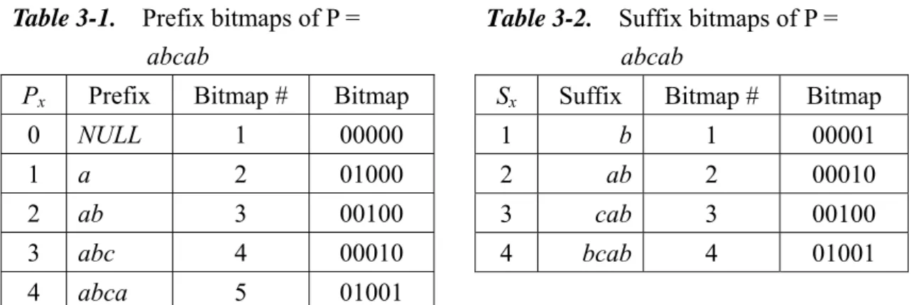
Example 1. Let P = abcab. Table 3-1 and Table 3-2 show the prefix bitmaps and
Chapter 3 An Efficient Pattern Matching Scheme In LZW Compressed Sequences
abca and = bcab. Consequently, we have = 4, = 4, and R = 01001. For this example, the first pattern occurrence starts at the first position of . In fact, as indicated by the two 1’s appeared in R, there are two pattern occurrences in .
2 S Px Sx 1 S 1 S S2
Table 3-1. Prefix bitmaps of P = abcab
Px Prefix Bitmap # Bitmap
0 NULL 1 00000
1 a 2 01000
2 ab 3 00100
3 abc 4 00010
4 abca 5 01001
Table 3-2. Suffix bitmaps of P = abcab
Sx Suffix Bitmap # Bitmap
1 b 1 00001
2 ab 2 00010
3 cab 3 00100
4 bcab 4 01001
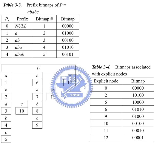
Example 2. Let P = ababc. Table 3-3 shows the prefix bitmaps of P. For ease of
description, we use the uncompacted suffix trie ST of P as illustrated in Figure 3-1. P
The bitmaps associated with the explicit nodes of ST are given in Table 3-4. As P
an example of query Q1, assume that = abab and the internal range I = [1, 2] (or [3,
4]) which represents substring = ab. In our implementation, I = [1, 2] (or [3, 4]) is represented by node 2 of the uncompacted suffix trie
1
S
2
S
P
ST . Since the prefix
number of S1 is 4 with corresponding prefix bitmap 00101 and the bitmap associated
with node 2 on ST is 10100, we have R = 00100. In other words, one pattern P
prefix starting at the third position of is found. As a result, the answer of query (4, [1, 2]) (or (4, [3, 4])) is (3-1) + | | = 2 + 2 = 4. As another example, if = ab and I = [2, 4] (the bitmap to be used is the one associated with node 9 of
1 S 1 Q Q1 S2 1 S ST ) P
which represents substring = bab, then we have = 2 and R = 00100 01000 =
00000. In this case, the answer of query Q
2
S Px ⊗
1(2, [2, 4]) is 2, which is the prefix
number of bab.
Let us consider now examples of query Q3. Assume that S1= ab which is
represented by node 2 of the uncompacted ST . If αP = b, then we have Q S3( , )1 α = [0, 0] because there is no transition from node 2 to any node with label b. However, if α= c, then we have Q S3( , )1 α = [1, 3] which is represented by node 10 of ST . P
Table 3-3. Prefix bitmaps of P = ababc
Px Prefix Bitmap # Bitmap
0 NULL 1 00000 1 a 2 01000 2 ab 3 00100 3 aba 4 01010 4 abab 5 00101 0 a b c 1 6 12 b a c 2 7 11 a c b 3 10 8 b c 4 9 c 5
Table 3-4. Bitmaps associated
with explicit nodes
Explicit node Bitmap
0 00000 2 10100 5 10000 6 01010 9 01000 10 00100 11 00010 12 00001
Figure 3-1. The uncompacted suffix trie STp of
P = ababc
3.2 Generalization to All Pattern Occurrences
As mentioned before, the pattern occurrence checking in the original ABF algorithm is only performed cross two consecutive data blocks. Moreover, only the
Chapter 3 An Efficient Pattern Matching Scheme In LZW Compressed Sequences
first occurrence is reported. To generalize the ABF algorithm to find all pattern occurrences, we need to consider all pattern occurrences cross two consecutive data blocks and those inside a data block as well. Our implementation presented in Chapter 3.1 allows detection of all pattern occurrences cross two consecutive data blocks. Therefore, the remaining work is to detect all pattern occurrences inside a data block. The generalization is designed to also report the absolute positions of pattern occurrences. Reporting the absolute positions of all occurrences may be desirable to some applications.
To detect all pattern occurrences inside a data block, we add two fields, called pattern inside flag (PIF) and pattern inside pointer (PIP), to every node of the LZW trie . The PIF flag is an indication of existence of patterns inside the chunk and the PIP pointer is used for backtracking to find the positions of all pattern occurrences inside the chunk. For the root node, its PIF is 0 and its PIP pointer points to the node itself, which is also 0. Assume that a new node M is to be added as a child node of node N. The PIP pointer of node M inherits the PIP value of node N if N is not a final node, i.e., a node whose chuck ends with the complete pattern P. To identify final nodes, we let the prefix number of a final node equal m. In case node N is a final node, the PIP pointer of node M points to node N. Similarly, the PIF of node M inherits the PIF value of node N unless the PIF of node N is 0 and node M is a final node. In this case, we set the PIF of node M to 1. With these additional fields, one can trace back the LZW trie to find all pattern occurrences inside a chuck. The trace-back ends once a node with PIP pointer points to the root node, i.e., PIP = 0, is reached. Note that although PIF can be replaced by the PIP pointer and the prefix number (PIF = 1 is equivalent to PIP
S
T
≠ 0 or prefix number = m), we suggest to use PIF to simplify the checking of pattern existence inside a chunk.
Note that, since we allow the prefix number of a node to be equal to m, we need to add to the set of prefix bitmaps an additional prefix bitmap corresponding to prefix number = m. The contents of the bitmap are assigned with the same algorithm described in Chapter 3.1. It is clear that the value of the variable Prefix may equal m too. However, it does not cause any error because the bitmap corresponding to prefix number = m is the same as the bitmap corresponding to prefix number = k, where pm k− +1...p is the longest suffix of P which is also a proper prefix of P, i.e., a m
prefix which is not P itself.
For convenience, we also allow the suffix number of a node to be equal to m. As a consequence, another bitmap corresponding to suffix number = m is added to the set of suffix bitmaps. Again, the contents of the added suffix bitmap are assigned according to the algorithm described in Chapter 3.1 and the additional suffix bitmap does not cause any error because a1i = 0 for all i, 1≤ i ≤ m+1.
To report absolute positions of pattern occurrences, we can rely on the depth
fields of nodes on the LZW trie and a global variable COUNT which stores the
number of bytes in text that have been scanned. Computation of the depth field is simple. The depth of the root node is 0. When node M is added as a child node of node N, the depth of node M equals that of node N plus one. Clearly, with the depth fields, one can compute the position of a node inside a chuck, which, together with the global variable COUNT, can be used to determine the absolute position of any pattern occurrence. The overall generalized algorithm is described below.
S
T S
Chapter 3 An Efficient Pattern Matching Scheme In LZW Compressed Sequences
A. Pattern Preprocessing
The prefix bitmaps and the suffix bitmaps are computed. Also, the compacted suffix trie ST of pattern P with the associated bitmaps are determined. P
B. Compressed Text Scanning
When constructing the LZW trie , each node’s node number, label, prefix
number, suffix number, internal range, the first symbol, depth, PIF, and PIP are computed and stored. The compressed text scanning procedure is described below.
S
T
Initialize: Prefix Å 0, COUNT Å 0 for l = 1 to n do
(Let node S.Z[l]’s prefix number = , suffix number = , internal range = I, PIF =
F and depth = D.)
x
P Sx
1 LZW Trie Construction
1.1 Add a new node numbered l+q to as a child node of S.Z[l]. Let α be
the label of node l+q.
S
T
1.2 The first symbol of node l+q is that of node S.Z[l].
1.3 The label of node l+q is the first symbol of node S.Z[l+1]. (If S.Z[l+1] =
l+q then the label is S.Z[l]'s first symbol.)
1.4 If S.Z[l] is an internal node with corresponding string S1
Set l+q's internal range [i, j] as Q S3( , )1 α . Else
Set l+q's internal range [i, j] as [0, 0].
1.5 If j = m, set l+q's suffix number as m-i+1. Otherwise, set l+q's suffix
number as Sx.
1.6 Set l+q's prefix number as Q P I , where 1( , )x α Iα is the internal range of α.
1.7 If F = 0 and l+q's prefix number = m, then l+q's PIF Å 1.
Else, l+q's PIF Å F.
1.8 Set the depth of node l+q as D+1. 1.9 If = m, then l+q's PIP Å S.Z[l]. Px
Else, l+q's PIP Å S.Z[l]’s PIP.
2 Pattern Search
If Sx ≠ 0
Check cross-boundary occurrences with the bitwise AND operation for query
Q2(Prefix,Sx). Let R = r r r1 2...m be the result of the bitwise AND operation.
for k = 1 to m do If rk = 1
Report the position: COUNT – k + 2 If F = 1 // Pattern is inside S.Z[l]
If Px = m
Report the position: COUNT + D – m + 1
N Å S.Z[l]’s PIP
While N ≠ 0
Report the position: COUNT + Dep(N) – m + 1
N Å N’s PIP
Prefix Å Q1(Prefix,I) // Note that the answer of Q1(Prefix,I) is , if the result of
bitwise AND operation for Q
x
P
1(Prefix,I) is all-zero
COUNT Å COUNT + D
The following example illustrates the process to detect all pattern occurrences and report their absolute positions.
Chapter 3 An Efficient Pattern Matching Scheme In LZW Compressed Sequences
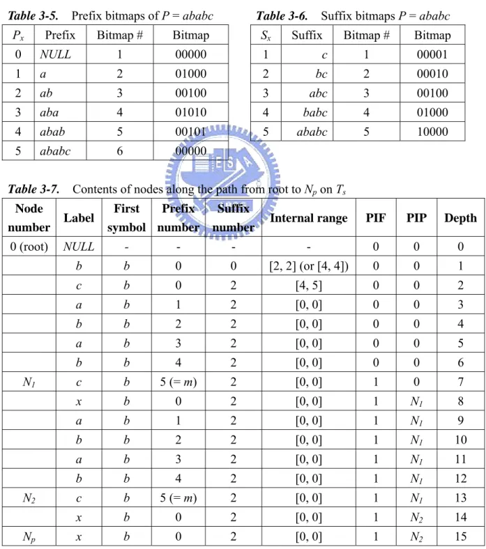
Example 3. As in Example 2, let P = ababc. The prefix bitmaps and the suffix
bitmaps are shown in Tables 3-5 and 3-6, respectively. Since the suffix trie of pattern P and the bitmaps associated with the explicit nodes are not changed, they are not reproduced here. Assume that some of the compressed text had been processed and the current value of COUNT = 100. Assume further that the last three chunks that had been processed are xxx, xxxx, and xaba, and the current chunk to be processed is Np= bcababcxababcxx.
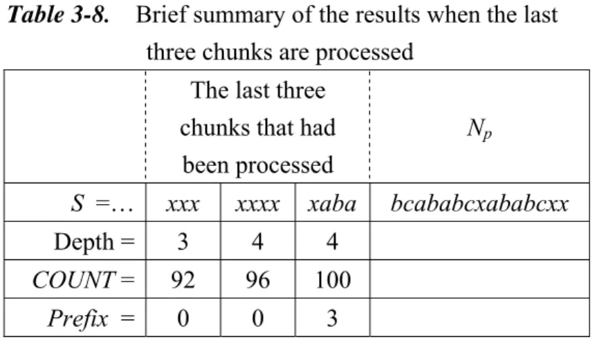
Table 3-7 shows the contents of the nodes along the path from the root node to node on the LZW tire. Note that there are two pattern occurrences inside the current chunk which can be determined by tracing back the PIP pointers. Table 3-8 shows a brief summary of the results when the last three chunks are processed. The procedure of pattern detection with report of absolute occurrence positions in
processing is sketched below.
p
N
p
N
• Reporting absolute positions of cross-boundary pattern occurrences: Since Np’s suffix number = 2 ≠ 0
// Check cross-boundary occurrences with bitmaps:
Prefix = 3 with corresponding bitmap 01010.
Np’s suffix number = 2 with corresponding bitmap 00010.
The result of bitwise AND operation R = 01010⊗ 00010 = 00010.
Î The absolute occurrence position COUNT – 4 + 2 = 98 is reported.
• Reporting absolute positions of inside-chunk pattern occurrences: Since Np’s PIF = 1
Since Np’s PIP = N2 ≠ 0
The absolute occurrence position COUNT + Dep(N2) – m + 1 = 109 is 21
reported.
Since N2’s PIP = N1 ≠ 0
The absolute occurrence position COUNT + Dep(N1) – m + 1 = 103 is
reported. Since N1’s PIP = 0
The trace-back ends.
Table 3-5. Prefix bitmaps of P = ababc
Px Prefix Bitmap # Bitmap
0 NULL 1 00000 1 a 2 01000 2 ab 3 00100 3 aba 4 01010 4 abab 5 00101 5 ababc 6 00000
Table 3-6. Suffix bitmaps P = ababc
Sx Suffix Bitmap # Bitmap
1 c 1 00001
2 bc 2 00010
3 abc 3 00100
4 babc 4 01000
5 ababc 5 10000
Table 3-7. Contents of nodes along the path from root to Np on Ts Node number Label First symbol Prefix number Suffix
number Internal range PIF PIP Depth
0 (root) NULL - - - - 0 0 0 b b 0 0 [2, 2] (or [4, 4]) 0 0 1 c b 0 2 [4, 5] 0 0 2 a b 1 2 [0, 0] 0 0 3 b b 2 2 [0, 0] 0 0 4 a b 3 2 [0, 0] 0 0 5 b b 4 2 [0, 0] 0 0 6 N1 c b 5 (= m) 2 [0, 0] 1 0 7 x b 0 2 [0, 0] 1 N1 8 a b 1 2 [0, 0] 1 N1 9 b b 2 2 [0, 0] 1 N1 10 a b 3 2 [0, 0] 1 N1 11 b b 4 2 [0, 0] 1 N1 12 N2 c b 5 (= m) 2 [0, 0] 1 N1 13 x b 0 2 [0, 0] 1 N2 14 Np x b 0 2 [0, 0] 1 N2 15
Chapter 3 An Efficient Pattern Matching Scheme In LZW Compressed Sequences
Table 3-8. Brief summary of the results when the last
three chunks are processed
The last three
chunks that had been processed Np S =… xxx xxxx xaba bcababcxababcxx Depth = 3 4 4 COUNT = 92 96 100 Prefix = 0 0 3 23
Chapter 4
Related Work
A different bitmap based implementation was independently developed by two groups of researchers [5] and [6]. The scheme proposed in [5] is more general than the one presented in [6] and thus we will follow its description and call it the Navarro-Raffinot (NR) scheme. As our generalization, the NR scheme can find all pattern occurrences and report their absolute positions. Below is a description of the NR scheme extracted from [5].
The NR scheme is a general technique to perform string matching when the text is presented as a sequence of atomic strings, called blocks, instead of a sequence of symbols. The blocks either have just one symbol or are formed by concatenating previously seen blocks. Let T' denote the text already processed at any moment of the search. When the search process is over, it holds that T' = T, the original text.
The blocks are processed one by one. For each new block B, a description for
B which has all the information of the block that is relevant for the search is computed.
This description is denoted by D(B) =(L, O, S, P, M), where
• L = |B|, the length of B in symbols
• O = Offs(B) = the length in symbols of the text we had processed when B
appeared
• S = Suff(B) = all the pattern positions which either start a complete occurrence
of B inside the pattern, or start a proper pattern suffix which matches with a prefix of B. Formally,
Suff(B) = {|x|, P = xBy} ∪ {|x|, |x| > 0 ∧ |z| > 0 ∧ P = xz ∧ B = zy}
• P = Pref(B) = all the pattern positions which either follow a complete occurrence
of B inside the pattern, or follow a proper pattern prefix which matches with a suffix of B. Formally,
Pref(B) = {|xB|, P = xBy ∧ |y| > 0} ∪ {|z|, |z| > 0 ∧ |y| > 0 ∧ P = zy ∧
_ Chapter 4 Related Work
• M = Matches(B) = all the block positions where the pattern occurs (Ø if |B| < |P|). Formally,
Matches(B) ={|x|, B = xPy}
Note that, to simplify the notation, the pattern positions start at zero in the above description, while in previous chapters, the pattern positions start at one.
There are two cases for a new block B: (a) the block is a symbol or (b) the block is a concatenation of other blocks previously known. For case (a), the description
D(B) can be obtained directly and, for case (b), it can be derived from the descriptions
of the previous blocks.
Once the description of the new block is computed, it is used to update the states of the search. This concludes the processing of a block and the search process moves to the next one. The states of the search contains the matches that have already occurred and the potential matches in progress, that is,
• Res(T') = the text positions that matched up to now. Formally, Res(T') = {|x|, T' = xPy}
• Active(T') = the set of positions following the pattern prefixes which match a suffix of the current text. Formally,
Active(T') = {|x|, |x| > 0 ∧ |y| > 0 ∧ P = xy ∧ T' = zx}
Hence, when the text processing is complete and T' is the whole text, Res(T) is the answer. The initial state of the search is Res(ε) = Active(ε) = Ø, and T' =ε, where ε denotes the empty string.
Four operations which are used in the search process are defined below [5].
• Lefti, which receives a set of Suff() positions not smaller than i, subtracts i to all
them and then adds new pattern positions filling the holes left by the shift. Formally,
Lefti(X) = {x−i, x∈X} ∪ {m−i, m−i+1, …., m−1}
• Righti, which does the same for Pref() positions, in the other direction.
Formally,
Righti (X) = {x+i, x∈X} ∪ {1,2, …., i}
• Addi(X) = {i + x, x∈X}, which adds i to all the elements of the set.
• Subtri(X) = {i − x, x∈X}, which subtracts all the elements of the set from i.
The base case of the scheme is to obtain the description of a block which is a symbol a. We have
• |B| = 1
• Offs(B) = |T'|
• Suff(B) = {|x|, P = xay}
• Pref(B) = {|xa|, P = xay ∧ |y| > 0} • Matches(B) = if P = a then {0} else Ø
which are direct applications of the general formulas.
Assume that block B is defined as the concatenation of one or more previous blocks. If B is identical to one previous block B', we just copy the description of B' for B. Assume that B is a concatenation of two blocks B1 and B2. Note that it
suffices to study concatenation of two blocks because the case of more than two blocks is a simple iteration over this procedure. We have to obtain the description for their concatenation D(B) = D(B1B2) = D(B1) · D(B2) (where · is a notation for
concatenation of block descriptions). The formulas were given in [5] as follows
• |B| = |B1| + |B2|
• Offs(B) = |T'|
• Suff(B) = Suff(B1) ∩ Left|B1|(Suff(B2))
• Pref(B) = Pref(B2) ∩ Right|B2| (Pref(B1))
• Matches(B) = Matches(B1) ∪ Add|B1|(Matches(B2))
∪ (Subtr|B1|(Pref(B1) ∩ Suff(B2)) ∩ {0, 1, 2,…., |B|−m})
We need to update the states of the search after processing a new block B. The formulas to obtain the new Res(T'B) and Active(T'B) values from the old Res(T') and Active(T') ones are
• Active(T'B) = Right|B|(Active(T')) ∩ Pref(B)
• Res(T'B) = Res(T') ∪ Add|T'|(Matches(B))
_ Chapter 4 Related Work The above searching technique can be easily realized with two sets of bitmaps, Pref(B) and Suff(B), for every block B. The length of every bitmap for Pref(B) and Suff(B) is equal to m, the pattern length. Obviously, for LZW compressed sequences, the number of bitmaps for Pref(B) and Suff(B) is the same as the number of nodes on the LZW trie. This number tends to be large for a big file. The states of the search, i.e., Res(T') and Active(T'), and the result of each block B, i.e., Matches(B), can be represented by either bitmaps or arrays of numbers. In the comparison presented in Chapter 5, we assume that Active(T') is represented by an m-bit bitmap and Res(T') and Matches(B) are represented by arrays of numbers. The reason to represent Res(T') as an array of numbers is that it is more space efficient because the number of pattern occurrences is usually much smaller than the file size. The reason to represent Matches(B) as an array of numbers is simply because the length of block B is not fixed.
Chapter 5
Comparison and Experimental Results
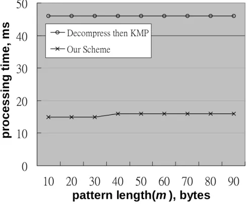
In this chapter, we compare the performance of our generalized algorithm with the one that performs decompression followed by pattern searching with the KMP algorithm [8]. The algorithms were implemented in C++ and the experiments were carried out on a PC with an AMD Athlon XP 1800+ CPU operated at 1.15GHz with 224MB of RAM running Microsoft Windows XP operating system. In the first test case, we use dosx.exe (an executable file in Windows) as our text which contains no pattern at all. The uncompressed size of dosx.exe is 53856 bytes. In the second test case, we insert various numbers of patterns with m = 4 in dosx.exe at randomly selected positions. The experimental results of test cases 1 and 2 are shown in Figures 5-1 and 5-2, respectively. As one can see, in comparison with the decompress-then-search algorithm, our proposed generalized algorithm has significantly better performance as expected. The performance of the NR scheme is very close to that of our generalized algorithm and thus is not shown in the figures. However, we can compare the space requirements of our generalized algorithm and the NR scheme.
______________ _ Chapter 5 Comparison and Experimental Results
0
10
20
30
40
50
10
20
30
40
50
60
70
80
90
pattern length(m ), bytes
pr
oc
es
s
ing t
im
e
, m
s
Decompress then KMP Our SchemeFigure 5-1. Performance comparison for test case 1
0
50
100
150
200
250
1 10 20 30 40 50 60 70 80 90 100
number of pattern occurrences(r )
pr
ocessi
ng t
im
e
, m
s
Decompress then KMP Our SchemeFigure 5-2. Performance comparison for test case 2
In our generalized algorithm, the number of bitmaps, including prefix bitmaps, suffix bitmaps, and the bitmaps associated with the nodes on the compacted suffix trie
P
ST is O(m). The LZW trie takes space O(t), where t is the number of nodes on . The prefix number, the suffix number, and the internal ranges stored in every node of are replaced by three pointers, each of size O( ) bits, which point to the appropriate bitmaps. Therefore, the space complexity of our generalized algorithm is O(m+t). For the NR scheme, the space complexity is O(t+r), where r is the number of pattern occurrences in text . Each of the O(t) descriptions contains five elements, L, O, S, P and M. Hence, there are O(t) bitmaps of S and O(t) bitmaps of P, each of the bitmaps has size m bits. Clearly, the space requirement of these two sets of bitmaps increases proportional to the size of the LZW trie. Another significant difference between the NR scheme and our generalized scheme is that the number of pattern occurrences r affects the space requirement of the NR scheme, but not ours. This effect will be studied later. Since the element O is not necessary for every node, we assume that it is omitted and instead a global counter COUNT is adopted in comparison. S T S T S T log m2 S
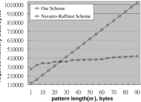
We ignore the space requirement of the NR scheme caused by r, that is, we intentionally let r = 0, in the third test case. The text used in test case 3 is dfrgntfs.exe (an executable file in Windows) whose uncompressed size is 104960 bytes. Comparison of the space requirements of our generalized scheme and the NR scheme for test case 3 is shown in Figure 5-3. It can be seen from the curves that our generalized scheme requires less storage than the NR scheme does if the pattern length is longer than 25.
______________ _ Chapter 5 Comparison and Experimental Results
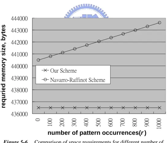
patterns inserted) of uncompressed size 296126 bytes and case5.txt (another randomly generated text file with 18000 patterns inserted) of uncompressed size 1705714 bytes as the texts, respectively. Figures 5-4 and 5-5 show, respectively, the space requirements under these two test cases for different pattern lengths. The NR scheme requires significantly more memory space than our generalized scheme, especially for long patterns. In Figure 5-6, we show the space requirements for pattern length m = 25 with various numbers of patterns inserted in dfrgntfs.exe. The uncompressed size of the modified dfrgntfs.exe is 249860 bytes. As one can see, the space requirement of the NR scheme increases as r increases while the space requirement of our generalized scheme is insensitive to the value of r.
110000
210000
310000
410000
510000
610000
710000
810000
910000
1010000
1
10
20
30
40
50
60
70
80
90
pattern length(m ), bytes
re
q
u
ir
ed
me
mo
ry
s
iz
e
, b
y
te
s
Our Scheme Navarro-Raffinot SchemeFigure 5-3. Comparison of space requirements for test case 3
40000
75000
110000
145000
180000
215000
250000
285000
320000
1
10
20
30
40
50
60
70
80
90
pattern length(m ), bytes
requi red m e mory size, byt e s Our Scheme Navarro-Raffinot Scheme
______________ _ Chapter 5 Comparison and Experimental Results
110000
160000
210000
260000
310000
360000
410000
460000
510000
1
10
20
30
40
50
60
70
80
90
pattern length(m ), bytes
req u ir ed memory si ze, by te s Our Scheme Navarro-Raffinot Scheme
Figure 5-5. Comparison of space requirements for test case 5
436000 437000 438000 439000 440000 441000 442000 443000 444000 0 100 200 300 400 500 600 700 800 900 1000
number of pattern occurrences(r )
re
qur
ied memor
y
size,
byt
e
s
Our Scheme Navarro-Raffinot SchemeFigure 5-6. Comparison of space requirements for different number of
pattern occurrences (m is fixed to be 25)
Chapter 6
Conclusion
We have presented in this thesis an efficient bitmap-based realization of the Amir-Benson-Farach algorithm for pattern search in LZW compressed sequences. The realization is then generalized to detect all pattern occurrences and report the absolute match positions. It is shown with experimental results that our proposed realization performs pattern search much faster than the decompress-then-search scheme. Moreover, compared with the Navarro-Raffinot scheme, another algorithm which can be realized with bitmaps, our proposed generalized algorithm requires less storage when the pattern is longer than 25 bytes. The difference could be huge if the number of pattern occurrences in the text is large. An interesting further research topic which is currently under investigation is to apply the idea of our design to pattern search with other compression techniques.
Bibliography
Bibliography
[1] Welch, T.A.: ‘A technique for High-Performance Data Compression’, June 1984, IEEE Computer, 17(6): 8-19
[2] Amir, A., Benson, G., and Farach, M.: ‘Let Sleeping Files Lie: Pattern Matching in Z-Compressed Files’, April 1996, Journal of Computer and System Sciences, vol. 52, pp. 299-307
[3] Tao, T., and Mukherjee, A.: ‘Pattern Matching in LZW Compressed Files’, August 2005, IEEE Transactions on Computers, vol. 54, no. 8, pp. 929-938
[4] Ho, M.H., and Yen, H.C.: ‘A Dictionary-based Compressed Pattern Matching
Algorithm’, IEEE Proceedings of the 26th Annual International Computer
Software and Applications Conference, Oxford, England, August 2002, pp. 873-878
[5] Navarro G., and Raffinot, M.: ‘A General Practical Approach to Pattern
Matching over Ziv-Lempel Compressed Text’, Proc. 10th Ann. Symp. on
Combinatorial Pattern Matching, Springer-Verlag, London, UK, 1999, Lecture Notes in Computer Science, vol. 1645, pp. 14-36
[6] Kida, T., Takeda, M., Shinohara, A., and Arikawa, S.: ‘Shift-And Approach to Pattern Matching in LZW Compressed Text’, Proc. 10th Ann. Symp. on
Combinatorial Pattern Matching, Springer-Verlag, London, UK, 1999, Lecture Notes in Computer Science, vol. 1645, pp. 1–13
[7] Kida, T., Takeda, M., Shinohara, A., Miyazaki, M., and Arikawa, S.: ‘Multiple Pattern Matching in LZW Compressed Text’, 2000, J. Discrete Algorithms, vol. 1, no. 1, pp. 133-158
[8] Knuth, D.E., Morris, J.H., and Pratt, V.R.: ‘Fast Pattern Matching in Strings’, 1977, SIAM Journal on Computing, 6, (2), pp.323-350