無線感測網路之自動燈光控制系統

國

立

交

通

大

學

網路工程研究所

碩

士

論

文

無 線 感 測 網 路 之 自 動 燈 光

控制系統

Autonomous Light Control by Wireless Sensor and

Actuator Networks

研 究 生：呂哲彥

無線感測網路之自動燈光控制系統

Autonomous Light Control by Wireless Sensor and Actuator Networks

研 究 生：呂哲彥 Student：Che-Yen Lu

指導教授：曾煜棋、易志偉 Advisor：Yu-Chee Tseng、

Chih-Wei Yi

國 立 交 通 大 學

網 路 工 程 研 究 所

碩 士 論 文

A Thesis

Submitted to Institute of Network Engineering College of Computer Science

National Chiao Tung University in partial Fulfillment of the Requirements

for the Degree of Master

in

Computer Science

June 2009

Hsinchu, Taiwan, Republic of China

無線感測網路之自動燈光控制系統

學生：呂哲彥

指導教授：曾煜棋 教授

易志偉 教授

國立交通大學網路工程研究所碩士班

摘

要

近年來，無線感測網路已經被廣泛的使用在許多的領域中。此篇論文中，我

們提出了一個基於無線感測網路之自動燈光控制系統。系統藉由使用者身上配戴

燈光感測器之讀數，做為調控燈光的依據。本系統主要針對兩大目標，分別為滿

足使用者照明以及節能省電。依據照明範圍的不同，將照明設備分為全區照明以

及區域照明設備。且基於全區照明以及區域照明考量因素不同，本論文對於兩種

設備分別提出不同的解決方案。對於全區照明，我們提出兩種控制演算法來控制

全區照明設備；對於區域照明則提出可追蹤使用者閱讀面之智慧型檯燈。由於不

需要額外的定位媒介以及裝置，且能自動根據環境光源的變化作調整，因此我們

將本系統稱為「自動化」燈光調控系統。本論文中，我們提供實驗數據以及實作

雛形結果來驗證系統的可行性。

關鍵字： 智慧型建築、燈光控制、無線通訊、普及運算，無線感測網路以及

LED。

Autonomous Light Control by Wireless Sensor and Actuator Networks

student：Che-Yen Lu

Advisors：Prof. Yu-Chee Tseng

Prof. Chih-Wei Yi

Institute of Network Engineering

National Chiao Tung University

ABSTRACT

Recently, wireless sensor and actuator networks (WSANs) have been widely

discussed in many applications. In this paper, we propose an autonomous light control

system based on the feedback from light sensors carried by users. Our design focuses

on meeting users' preferences and energy efficiency. Both whole and local lighting

devices are considered. Users' preferences may depend on their activities and profiles

and two requirement models are considered: binary satisfaction and continuous

satisfaction models. For controlling whole lighting devices, two decision algorithms

are proposed. For controlling local lighting devices, a surface-tracking scheme is

proposed. Our solutions are autonomous because, as opposed to existing solutions,

they can dynamically adapt to environment changes and do not need to track users'

current locations. Simulations and prototyping results are presented to verify the

effectiveness of these results.

Keywords:

Intelligent building, light control, pervasive computing, wireless

誌

謝

首先，誠摯的感謝曾煜棋教授以及易志偉教授對於我碩士生涯兩年來的指導

與鼓勵，並且提供我良好的研究環境以及充足的實驗器材，讓我能夠順利的完成

此篇論文並且順利取得碩士學位。

此外，也由衷的感謝葉倫武學長以及廖家良助理。無論在論文研究與寫稿上，

葉倫武學長皆細心提供了我許多寶貴的建議以及指導。而在硬體實作以及佈建

上，廖家良助理也給予了我許多幫助。另外，我要感謝 HSCC 以及 NOL 實驗室的

全體成員，在我碩班兩年中的幫忙與鼓勵。

最後，感謝我的家人以及關心我的人對我的期許以及關懷，使我能夠無虞地

完成我的學業。

呂哲彥 於

國立交通大學網路工程研究所碩士班

中華民國九十八年六月

Contents

1 Introduction 1

2 System Model 4

2.1 Light Measurement Method . . . 4

2.2 Control Flow . . . 7

3 Control of Whole Lighting Devices 9 3.1 Binary Satisfaction Model . . . 9

3.2 Continuous Satisfaction Model . . . 10

3.3 Examples . . . 11

4 Control of Local Lighting Devices 14 5 Simulation Results 18 6 Prototyping Results 26 6.1 User Badge and Light Sensor . . . 26

6.2 Whole Lighting Device . . . 26

6.3 iLamp . . . 29

6.4 Control Host . . . 29

6.5 Performance Verification . . . 30

List of Figures

1.1 The network scenario of our system. . . 2

2.1 Measuring the impact of a light source Xj on a light sensor si. . . 5

2.2 An example of continuous satisfaction. . . 6

2.3 Light control flow chart. . . 7

3.1 An example for the binary satisfaction model. . . 11

3.2 An example of continuous satisfaction model. . . 12

4.1 Service scenario of an iLamp and a light sensor. . . 15

4.2 The geometry model of iLamp to track the location of si. . . 16

5.1 Requirement pools: (a) RP 1 and (b) RP 2. . . 20

5.2 Requirement pools: (a) RP 3 and (b) RP 4. . . 21

5.3 Comparison under the binary satisfaction model: (a) network sce-nario S1 and pool RP 1 and (b) network scesce-nario S1 and pool RP 2. . . 22

5.4 Comparison under the binary satisfaction model: (a) network sce-nario S2 and pool RP 1 and (b) network scesce-nario S2 and pool RP 2. . . 23

5.5 Comparison under the continuous satisfaction model: (a) network scenario S1 and pool RP 3 and (b) network scenario S1 and pool RP 4. . . 24

5.6 Comparison under the continuous satisfaction model: (a) network scenario S2 and pool RP 3 and (b) network scenario S2 and pool RP 4. . . 25

6.1 Hardware and software system architecture of our prototype. . . . 27

6.2 User badge, which looks like a bookmark. . . 28

6.3 Testing environment and a whole lighting device. . . 28

6.4 The demonstration of iLamp. . . 29

6.5 Comparison between ideal and real value with fixed candela. . . . 30

6.7 Interpolation under scenario of RP 1 and 3 users. . . 31 6.8 Comparison between implementation and simulation results. . . . 32

Chapter 1

Introduction

The rapid progress of wireless communication and embedded MEMS technolo-gies has made wireless sensor and actuator networks (WSANs) possible. A WSAN [10][11][20] is a distributed system consisting of sensor and actuator nodes interconnected by wireless links. Using sensed data from sensor nodes, actuators can perform actions accordingly. Applications of WSANs include smart living space [21], localization [13][15], and environmental monitoring [14][23].

Recently, WSANs have been applied to energy conservation applications such as light control [14][16][17][19][22]. Reference [22] uses wireless sensors to con-trol lighting devices according to daylight intensity. Reference [17] defines several user requirements and cost functions. The goal is to adjust lights to minimize the total cost. However, the result is mainly for media production. Considering light control is a trade-off between energy consumption and user satisfaction, refer-ence [19] applies the concept of utility to adjust illuminations so as to maximize the total utility. However, it does not consider the fact that people need different illuminations under different activities. In references [17] and [19], it needs to measure all combinations of dimmer settings and the resulting illuminations at all locations. If there are k interested locations, d dimmer levels, and m light-ing devices, the measurement complexity is O(kdm). With pervasive sensors, [16] further reduce the measuring time to O(km). The goal is to satisfy users’ demands while optimizing energy efficiency. These works all rely on knowing

Control Host

Whole Lighting Device User

Light Sensor Sink

Local Lighting Device

B A C E D a b c

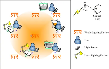
Figure 1.1: The network scenario of our system.

users’ current locations, so extra localization mechanisms are needed.

In this work, we propose a light control system that considers users’ prefer-ences and energy conservation. Fig. 1.1 shows the network scenario. Each user carries a light sensor and these sensors can help each other to relay their sensing data to the sink node. Then the control host can give commands to lighting de-vices. We consider LEDs [3][4] serving as whole and local lighting dede-vices. The former can provide background illuminations for multiple users in wide areas. The latter are similar to desk lamps to provide concentrated illuminations. For example, in Fig. 1.1, device a in the center can provide background illuminations for user B, C and E, and device b can only provide concentrated illumination for user B.

In our system, users may have different illumination requirements according to their activities and profiles. We distinguish from two types of requirements, background and concentrated ones. For example, in Fig. 1.1, user A is watch-ing television, B is readwatch-ing a book, and C is sleepwatch-ing. Both A and B require the same background illuminations, but B needs concentrated illumination, and C requires no background and concentrated illuminations. A user is said to be

satisfied if the provided background and concentrated illuminations fall into the required ranges. To evaluate the satisfaction level of a user, we further consider a binary satisfaction and a continuous satisfaction models. The former only returns a satisfaction value of 1 or 0, while the latter returns a value between 0 and 1. We develop two algorithms to adjust whole lighting devices for these models with the goals of meeting users’ requirements while minimizing energy consumption. In case that it is impossible to satisfy all users simultaneously, we will gradually relax users’ requirements until all users are satisfied. For concentrated illumina-tions, assuming that local lighting devices are moveable (which can be supported by robot arms), we develop a novel “surface-tracking” scheme to follow to local movements of users to provide required illuminations.

The main contributions of this work are twofold. First, our model is designed for “point-like” light sources, such as LEDs, which are more energy-efficient than traditional light sources and are expected to be the main lighting sources in the future. We show how to take advantage of its light propagation property to con-duct light control. Second, compared to existing solutions, our solution is “au-tonomous” in the sense that it can dynamically adapt to environment changes and does not need to track users’ current locations.

There rest of this work is organized as follows. Chapter 2 presents the system model. Chapter 3 and Chapter 4 introduce our control algorithms for background and concentrated light sources, respectively. Chapter 5 contains simulation re-sults. Chapter 6 presents our prototyping rere-sults. Conclusions are drawn in Chap-ter 7

Chapter 2

System Model

2.1 Light Measurement Method

In our system, there are n users, u1, u2, ..., un, m whole lighting devices, D1, D2,

..., Dm, and m0 local lighting devices, d1, d2, ..., dm0. These devices are all

con-trollable devices. Each user uicarries a light sensor si, which periodically reports

its sensed illumination level Pito the control host. The current luminous intensity

emitted by Di is denoted by CiD, and that by di is denoted by Cid. Considering

physical limitations, we assume that CD

i and Cid should satisfy CiDmin ≤ CiD ≤

CDmax

i and Cidmin≤ Cid≤ Cidmax.

We make the following assumptions in our work. First, there exists natural light source, but it may change over time. Second, light sources are assumed to be “point-like” ones such as LEDs. This makes modeling the impact of light sources easier. For whole lighting sources, disturbance from other objects may exist (such as furniture, obstacles, walls, etc.). However, we assume that it is possible to derive the impact of a whole lighting device on a sensor, while allows us to decide the proper intensity of each light source. For local lighting sources, we assume that no such disturbance exists. This allows us to measure the distance between a lighting source and a user. In fact, we even assume that local lighting sources are supported by robot arms and thus they may be moved around to focus to particular places. We will discuss more about this in Chapter 4.

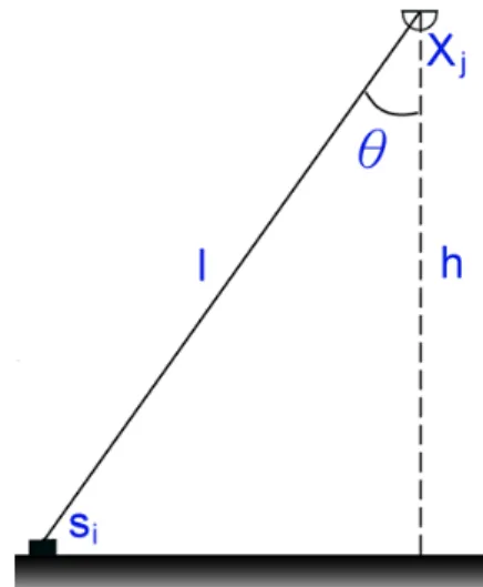
Figure 2.1: Measuring the impact of a light source Xj on a light sensor si.

Next, we explain how to model the impact of a light source Xj on a light

sensor si (refer to in Fig. 2.1). Xj can be a whole lighting source Dj or a local

lighting source dj. Let l and h be the distances from Xj to si and to the nearest

ground, respectively. Now let Xj increase its intensity by ∆CjX candela and we

measure the change of illumination ∆Li,j at si. According to the light propagation

property, ∆Li,j = ∆CX j × cos θ l2 = ∆CX j × h l3 . (2.1) From ∆CX

j and the observed ∆Li,j, we define the impact of Xj on sias

wX_i,j = ∆Li,j

∆CX

j

= h

l3 (2.2)

Intuitively, this implies that even if l and h are unknown, we can still measure wX

i,j from ∆CjX and ∆Li,j. Therefore, we can easily decide the amount of

in-crement/decrement on X0

js intensity to achieve the desired level of illumination

sensed by si. Below, when Xj = Dj, the impacted is written as wi,jD; when

Xj = dj, it is written as wi,jd . The measurement of impact values should be done

0 0.2 0.4 0.6 0.8 1 0 100 200 300 400 500 600 700 800 555 245 Satisfaction value

Sensed illumination (Lux)

Threshold Illumination interval

Threshold Illumination interval

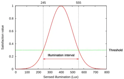
Figure 2.2: An example of continuous satisfaction.

consider only measuring the impacts of some light devices and use interpolation techniques to estimate those unknown impact values to further reduce the mea-surement cost. In comparison, this is much lower than that of [16], [17] and [19].

Because illuminations are additive [19], the Pi sensed by si is the sum of the

natural light Lna

i and the illuminations provided by whole and local lighting

de-vices Pi ≈ m X j=1 (wD i,j× CiD) + m0 X j=1 (wd i,j × Cid) + Lnai . (2.3)

Pi can be considered as the concentrated illumination perceived by ui and the

background illumination perceived by uican be estimated by Pi−

P_m0

j=1(wi,jd × Cid).

In this work, we consider two kinds of user model for background illuminations:

1. Binary Satisfaction Model: Each user ui has a acceptable concentrated

il-lumination interval [Rcl

i , Rcui ] and an acceptable background illumination

interval [Rbl

i , Ribu]. The user is said to be satisfied if its concentrated and

background illuminations fall within these intervals, respectively.

back-Binary Satisfaction Model Whole light control

Weight Measurement

User movement or user requirement is unsatisfied ?

Continuous Satisfaction Model

Intelligent Lamp Local light control Yes

No

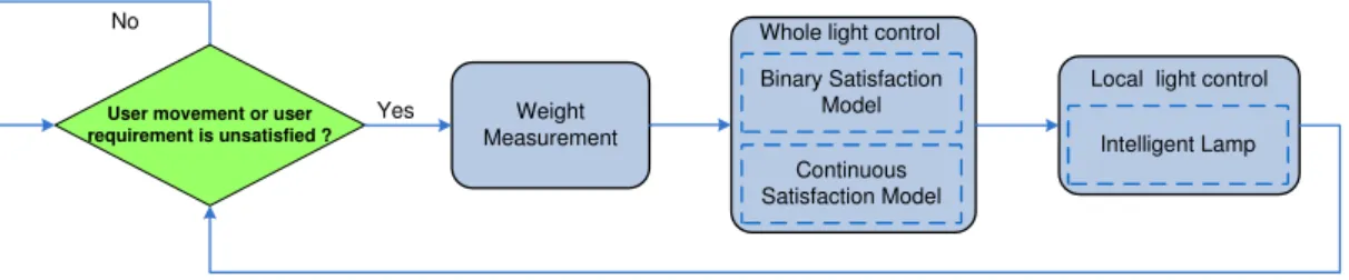
Figure 2.3: Light control flow chart.

ground illumination requirements, but they are specified by utility-like

func-tions as in [19]. The former has a mean µc

i, a variance value σci, and a

threshold tc

i. The latter has a mean µbi, a variance value σbi, and a threshold

tb

i are specified. Given a concentrated illumination x, ui has a satisfaction

value of fc

i(x) = exp(

−(x−µc i)2 2(σc

i)2 ) and a acceptable concentrated illumination

interval [µc i − σic p −2ln(tc i), µci + σci p −2ln(tc

i)]. Similarly, given a

back-ground illumination x, ui has a satisfaction value of fib(x) = exp(

−(x−µb i)2 2(σb

i)2 )

and a acceptable background illumination interval [µb

i−σib p −2ln(tb i), µbi+ σb i p −2ln(tb

i)]. Fig. 2.2 shows an example of continuous model with µ =

400, σ = 100, and t = 0.3.

Note that for concentrated illuminations, we assume that it is always possible to meet users’ requirements since local lighting devices are very close to users, so no particular model is specified.

2.2 Control Flow

Fig. 2.3 show the light control flow of our system. It is triggered by user move-ment, periodical check, or inputs from sensors which reflect that some users are

not satisfied. The weight measurement block will determine wD

i,j and wi,jd is

dis-cussed in Section 2.1. Then the whole light control and the local light control

modules will follow. We will use Pi and Pi −

P_m

j=1(wdi,j× Cid) to measure the

Cd

is to achieve our goal. It turns out that decisions of whole or local light control

Chapter 3

Control of Whole Lighting Devices

Under the binary model, we propose to minimize the total energy cost. Under the continuous model, since there is a satisfaction value associated with each user, we propose to maximize users’ total satisfaction value.

3.1 Binary Satisfaction Model

Our goal is to determine an amount of adjustment ∆CD

i on CiD for device Di to

meet users’ background illumination requirements. Under the binary satisfaction

model, we are given the inputs: (1) CD

1 , C2D, . . . , CmD, (2) C1d, C2d, . . . , Cmd, and (3)

P1, P2, . . . , Pn. Also, from the light measurement method in Section 2.1, we can

derive: (1) wD

1,1, wD1,2, . . . , wDn,m, (2) wd1,1, w1,2d , ..., w_n,md 0, and (3) Lna₁ , Lna₂ , . . . , Lna_n .

Our goal is to solve ∆CD

1 , ∆C2D, . . . , ∆CmD with the objective function:

min m X i=1 (CD i + ∆CiD) (3.1) subject to: Rbl_i ≤ m X j=1

w_i,jD × (C_jD + ∆C_jD) + Lna_i ≤ R_ibu for all i = 1 . . . n (3.2)

CDmin

i ≤ CiD+ ∆CiD ≤ CiDmax for all i = 1 . . . m (3.3)

Eq. (3.1) is to minimize the total power consumption of whole lighting de-vices. Eq. (3.2) imposes that all users’ background illumination requirements

should be met. Eq. (3.3) is to confine the adjustment result within the maximum and the minimum bounds. This is a linear programming problem and can be solved by the Simplex method [9]. However, in reality, there may not exist feasi-ble solutions. In this case, we will gradually relax users’ requirements to make this problem feasible. Reference [18] already shows that finding a feasible subsystem of a linear system by eliminating the fewest constraints is NP-hard. Therefore, we propose an iterative process as follows: First, we run the Simplex method. If no

feasible solution is found, we change ui’s requirement to [Rbli − α, Rbui + α] for

each i = 1...n, where α is a constant. Then we run the Simplex method again. This is repeated until a solution is found.

3.2 Continuous Satisfaction Model

Under this model, the inputs are: (1) CD

1 , C2D, . . . , CmD, (2) C1d, C2d, . . . , Cmd, and

(3) P1, P2, . . . , Pn. Again, we can derive: (1) wD1,1, wD1,2, . . . , wDn,m, (2) w1,1d , w1,2d , . . . , w_n,md 0,

and (3) Lna

1 , Lna2 , . . . , Lnan . The goal is to solve ∆C1D, ∆C2D, . . . , ∆CmD with the

objective function: max n X i=1 fb i( m X j=1 wD i,j× (CjD+ ∆CjD) + Lnai ) (3.4) subject to: µb i − σbi q −2ln(tb i) ≤ m X j=1 wD i,j× (CjD+ ∆CjD) + Lnai ≤ µb_i + σ_ib q −2ln(tb i) for all i = 1 . . . n (3.5) CDmin

i ≤ CiD + ∆CiD ≤ CiDmax for all i = 1 . . . m (3.6)

Eq. (3.4) is to maximize the sum of satisfaction values of all users. Eq. (3.5) imposes that all users’ background illumination requirements should be met. Eq. (3.6) specifies the bounds. This is a non-linear programming problem and can be solved by a sequential quadratic programming (SQP) method [8]. When there is no

fea-1 2 0.2 2 1 0.1 0.3 0.15

150

1 na

L

150

2 na

L

2000

max 1 D

C

max

₂₀₀₀

2 D

C

>

R

₁bl

,

R

₁bu

@

>

300

,

500

@

>

_,

@

>

₄₀₀

_,

₆₀₀

@

2 2 bu bl

R

R

3

.

0

2 , 1 D

w

1

.

0

1 , 1 D

w

15

.

0

2 , 2 D

w

2

.

0

1 , 2 D

w

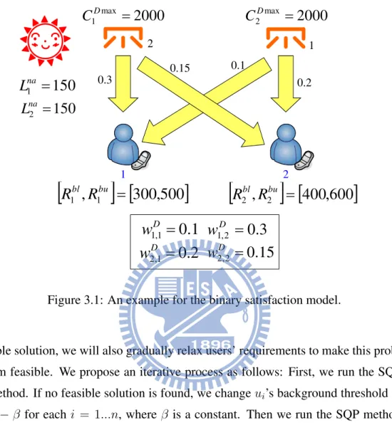
Figure 3.1: An example for the binary satisfaction model.

sible solution, we will also gradually relax users’ requirements to make this prob-lem feasible. We propose an iterative process as follows: First, we run the SQP

method. If no feasible solution is found, we change ui’s background threshold to

tb

i − β for each i = 1...n, where β is a constant. Then we run the SQP method

again. This is repeated until a solution is found.

3.3 Examples

For the binary satisfaction model, Fig. 3.1 shows a scenario with users u1and u2,

devices D1and D2, and natural light Lna1 = 150 and Lna2 = 150. Let [Rbl1, Rbu1 ] =

[300, 500] and [Rbl

1 2 0.2 2 1 0.1 0.3 0.15

150

1 na

L

150

2 na

L

2000

max 1 D

C

max

₂₀₀₀

2 D

C

3

.

0

2 , 1 D

w

1

.

0

1 , 1 D

w

15

.

0

2 , 2 D

w

2

.

0

1 , 2 D

w



P

₁D

,

V

₁D

,

t

₁D



>

500

,

100

,

0

.

3

@



_,

_,



>

₄₅₀

_,

₁₅₀

_,

₀

_.

₃

@

2 2 2 D D D

t

V

P

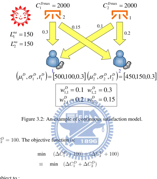
Figure 3.2: An example of continuous satisfaction model.

CD

2 = 100. The objective function is:

min (∆CD 1 + 100) + (∆C2D+ 100) ≡ min (∆CD 1 + ∆C2D) subject to : 300 ≤ 150 + 0.1 × (100 + ∆CD 1 ) + 0.3 × (100 + ∆C2D) ≤ 500 400 ≤ 150 + 0.2 × (100 + ∆CD 1 ) + 0.15 × (100 + ∆C2D) ≤ 600 0 ≤ (100 + ∆C₁D) ≤ 2000 0 ≤ (100 + ∆CD 2 ) ≤ 2000

Because this problem is feasible, the solution is ∆CD

1 = 1066.67 and ∆C2D =

For continuous satisfaction model, Fig. 3.2 also shows a scenario with users

u1 and u2, devices D1 and D2, current intensities C1D = 100 and C2D = 100,

and natural light Lna

1 = 150 and Lna2 = 150. We assume that (µb1, σb1, tb1) =

(500, 100, 0.3) and (µD

2, σ2D, tb2) = (450, 150, 0.3) for u1 and u2, respectively.

Given tb

1 = 0.3 and tb2 = 0.3, we can derive [µb1−σ1b

p −2ln(tb 1), µbi+σib p −2ln(tb i)] = [345, 655] and [µb 2 − σ2b p −2ln(tb 2) , µb2+ σ2b p −2ln(tb 2)] = [167, 633] for u1 and

u2, respectively. The objective function is:

max fb 1 ¡ 150 + 0.1 × (100 + ∆CD 1 ) + 0.3 × (100 + ∆C2D) ¢ + f₂b¡150 + 0.2 × (100 + ∆C₁D) + 0.15 × (100 + ∆C₂D)¢ subject to: 345 ≤ 150 + 0.1 × (100 + ∆CD 1 ) + 0.3 × (100 + ∆C1D) ≤ 655 167 ≤ 150 + 0.2 × (100 + ∆C₂D) + 0.15 × (100 + ∆C₂D) ≤ 633 0 ≤ (100 + ∆CD 1 ) ≤ 2000 0 ≤ (100 + ∆CD 2 ) ≤ 2000.

Again, this problem is also feasible. The solution is ∆CD

1 = 255.4 and ∆C2D =

Chapter 4

Control of Local Lighting Devices

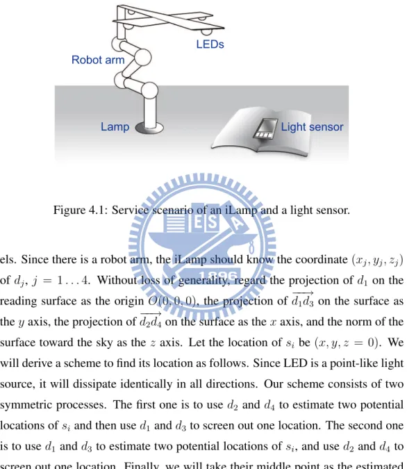
The above results are able to adjust background illuminations to meet users’ needs. In this chapter, we propose a robotic device, called Intelligent Lamp (iLamp) to provide concentrated illuminations. Each iLamp has a robot arm with at least four local lighting devices and is supposed to serve one user who has concentrated illumination need at a time. The service scenario is shown in Fig. 4.1. The sensor should be placed on the reading surface. On detecting a user under its service area, the iLamp will compute its relative location to the light sensor, move via its robot arm to a better location, and then adjust its luminous intensities to meet the need with the least energy. Detecting a nearby user is a simple job since a local lighting device can check if it has non-negative impact on a sensor.

Given an iLamp and a light sensor si, they will cooperate with each other by

the following four steps to achieve our goal: (1) collect the current Pi sensed by

si, (2) calculate the location of si, (3) adjust the lamp’s robot arm, and (4) adjust

the luminous intensities of its lighting devices. Step 1 is executed periodically. Once it finds that the current illumination falls outside the required interval, steps 2, 3, and 4 are triggered. Central to our scheme is step 2, so we will elaborate it in more details below.

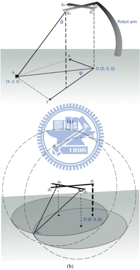
To drive step 2, assume for simplicity that the iLamp has four local lighting

devices d1, d2, d3, and d4as shown in the geometry model in Fig. 4.2(a). Note that

mod-Figure 4.1: Service scenario of an iLamp and a light sensor.

els. Since there is a robot arm, the iLamp should know the coordinate (xj, yj, zj)

of dj, j = 1 . . . 4. Without loss of generality, regard the projection of d1 on the

reading surface as the origin O(0, 0, 0), the projection of −−→d1d3 on the surface as

the y axis, the projection of−−→d2d4 on the surface as the x axis, and the norm of the

surface toward the sky as the z axis. Let the location of si be (x, y, z = 0). We

will derive a scheme to find its location as follows. Since LED is a point-like light source, it will dissipate identically in all directions. Our scheme consists of two

symmetric processes. The first one is to use d2 and d4 to estimate two potential

locations of siand then use d1 and d3 to screen out one location. The second one

is to use d1 and d3 to estimate two potential locations of si, and use d2 and d4 to

screen out one location. Finally, we will take their middle point as the estimated

location of si.

1. For each dj, j = 1 . . . 4, increase its luminous intensity by ∆Cjcandela and

Accord-(a)

(b)

ing to the definition of illumination, we have the equality: ∆Lij = ∆Cj× cos θij (p(x − xj)2+ (y − yj)2+ (z − zj)2)2 , where cos θij = zj p (x − xj)2+ (y − yj)2+ (z − zj)2 . This leads to ∆Lij = ∆Ci× zj (p(x − xj)2+ (y − yj)2+ (z − zj)2)3 . (4.1)

2. Observe that the equations for ∆Li2 and ∆Li4represent two balls centered

at d2 and d4, respectively. Since it is known that z = 0, each of these two

balls intersects with plane z = 0 at a circle. These two circles will intersect

at two points. Using any equation for ∆Li1and ∆Li3, we can pick one point

as the estimated location of si, called e1. (Refer to Fig. 4.2(b).)

3. Similarly, the equations for ∆Li1and ∆Li3represent two balls at d1and d3,

respectively, each intersecting with plane z = 0 at a circle. Again, these two circles intersect at two points, and we can pick one point as the location of

si, call e2, with the assistance of ∆Li2and ∆Li4.

4. Finally, the location of si is predicted as the middle point of e1 and e2.

In step 3, we will move our lighting devices toward the upper side of si. This

includes two sub-steps. First, we will rotate the robot arm by φ angle such that the

vector from d1to d3, after projecting to the reading surface, is pointing toward the

location of si. Second, it moves to the upper side of si to provide a proper reading

angle (a typical angle is 60◦_).

Step 4 is to adjust Cd

j, j = 1 . . . 4 to meet the concentrated illumination

de-mand of ui. From the results in Chapter 3, some background and natural

illumi-nations have already been provided. So we only need to add some more light to

meet ui’s need. The results in Chapter 3 can be directly applied again here, so we

Chapter 5

Simulation Results

To understand how our schemes for whole lighting control meet users’ require-ments whole save energy. We have developed a simulator. Two scenarios are

considered. Scenario S1 is a room of size 10 × 10m2 _{with 5 × 5 whole lighting}

devices. Scenario S2 is a room of size 20 × 20m2_{with 9 × 9 devices. Both deploy}

devices as grids. We set all CDmin

i = 0 and all CiDmax = 3000. We compare with

two schemes. The FIX scheme is a very intuitive one assuming that the users’ locations are known in advance, we always pick the nearest devices and set them to fixed candela value n. We denote this scheme as FIX-n below. The GREEDY scheme also assumes that users’ locations are known; for each user, it picks the nearest device to satisfy the user (if possible). If it still lacks of illumination, the second nearest device is picked to increase its intensity. This is repeated until the user is satisfied. Note that it may happen that a user is satisfied first but later on becomes unsatisfied due to other devices change their intensities. Below, we verify both our models.

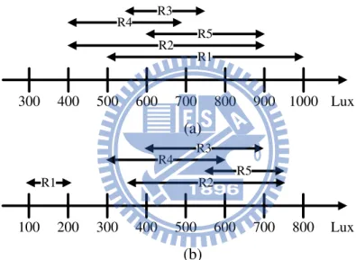
• Binary Satisfaction Model: We consider two requirement pools, RP 1 and RP 2, as shown in Fig. 5.1. Each range Riin Fig. 5.1 represents an expected

illumination interval. A user will randomly one Ri as its requirement. We

consider two performance indices here. The first index is the total energy consumption. The second index is called, which reflects the difference

is: GAP (ui) = ½ 0 if Rbl i ≤ Pi ≤ Rbui min(|Rbl i − Pi|, |Rbui − Pi|) otherwise (5.1)

We will measure the average GAP of all users.

Fig. 5.3 and Fig. 5.4 show our simulation results under different combina-tions of S1/S2 and RP 1/RP 2. In Fig. 5.3 (a), we see that our scheme is most energy-efficient while keeps the average GAP close to zero. This is because the requirement intervals in RP 1 have common overlapping, which allows our system to satisfy all users in most cases. Note that although FIX-1000 uses less energy, its GAP is much larger. Fig. 5.3 (b) adopts RP 2. Be-cause some requirements are violated, our scheme also induces some gaps. However, our scheme is most energy-efficient. Fig. 5.4 considers S2 and the trends are similar. This demonstrates that our scheme is quite scalable to network size.

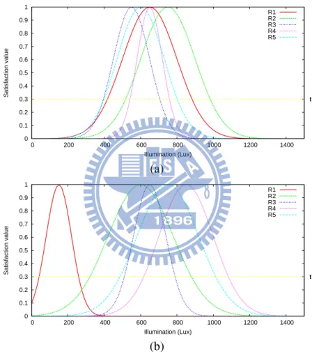
• Continuous Satisfaction Model: We define two requirement pools RP 3 and RP 4, as shown in Fig. 5.2. Note that RP 4 has higher deviation in require-ments than RP 3. The satisfaction threshold t is set to 0.3. We compare two performance indices: average user satisfaction and energy consump-tion. Fig. 5.5 and Fig. 5.6 show out simulation results under different com-binations of S1/S2 and RP 3/RP 4. These results consistently indicate that our scheme provides the highest satisfaction levels and outperforms FIX and GREEDY schemes in energy consumption.

300 400 500 600 700 800 900 1000 R2 R1 R4 R3 R5 Lux (a) 100 200 300 400 500 600 700 800 R1 R5 R2 R3 R4 Lux (b)

0 0.1 0.2 0.3 0.4 0.5 0.6 0.7 0.8 0.9 1 0 200 400 600 800 1000 1200 1400 Satisfaction value Illumination (Lux) tt R1 R2 R3 R4 R5 (a) 0 0.1 0.2 0.3 0.4 0.5 0.6 0.7 0.8 0.9 1 0 200 400 600 800 1000 1200 1400 Satisfaction value Illumination (Lux) tt R1 R2 R3 R4 R5 (b)

0 5000 10000 15000 20000 25000 30000 35000 40000 45000 40 35 30 25 20 15 10 5

Average energy consumption (lumen)

Number of users binary model GREEDY FIX-2000 FIX-1500 FIX-1000 0 50 100 150 200 250 300 350 400 450 40 35 30 25 20 15 10 5

Average GAP (lux)

Number of users binary model GREEDY FIX-2000 FIX-1500 FIX-1000 (a) 0 5000 10000 15000 20000 25000 30000 35000 40000 40 35 30 25 20 15 10 5

Average energy consumption (lumen)

Number of users binary model GREEDY FIX-2000 FIX-1500 FIX-1000 0 100 200 300 400 500 600 40 35 30 25 20 15 10 5

Average GAP (lux)

Number of users binary model GREEDY FIX-2000 FIX-1500 FIX-1000 (b)

Figure 5.3: Comparison under the binary satisfaction model: (a) network scenario S1 and pool RP 1 and (b) network scenario S1 and pool RP 2.

0 20000 40000 60000 80000 100000 120000 80 70 60 50 40 30 20 10

Average energy consumption (lumen)

Number of users binary model GREEDY FIX-2000 FIX-1500 FIX-1000 0 100 200 300 400 500 600 80 70 60 50 40 30 20 10

Average GAP (lux)

Number of users binary model GREEDY FIX-2000 FIX-1500 FIX-1000 (a) 0 10000 20000 30000 40000 50000 60000 70000 80000 90000 100000 80 70 60 50 40 30 20 10

Average energy consumption (lumen)

Number of users binary model GREEDY FIX-2000 FIX-1500 FIX-1000 0 100 200 300 400 500 600 700 80 70 60 50 40 30 20 10

Average GAP (lux)

Number of users binary model GREEDY FIX-2000 FIX-1500 FIX-1000 (b)

Figure 5.4: Comparison under the binary satisfaction model: (a) network scenario S2 and pool RP 1 and (b) network scenario S2 and pool RP 2.

0 5000 10000 15000 20000 25000 30000 35000 40000 45000 40 35 30 25 20 15 10 5

Average energy consumption (lumen)

Number of users continuous model GREEDY FIX-2000 FIX-1500 FIX-1000 0 0.1 0.2 0.3 0.4 0.5 0.6 0.7 0.8 0.9 40 35 30 25 20 15 10 5 Average satisfaction Number of users continuous model GREEDY FIX-2000 FIX-1500 FIX-1000 (a) 0 5000 10000 15000 20000 25000 30000 35000 40000 40 35 30 25 20 15 10 5

Average energy consumption (lumen)

Number of users continuous model GREEDY FIX-2000 FIX-1500 FIX-1000 0 0.1 0.2 0.3 0.4 0.5 0.6 0.7 0.8 40 35 30 25 20 15 10 5 Average satisfaction Number of users continuous model GREEDY FIX-2000 FIX-1500 FIX-1000 (b)

Figure 5.5: Comparison under the continuous satisfaction model: (a) network scenario S1 and pool RP 3 and (b) network scenario S1 and pool RP 4.

0 20000 40000 60000 80000 100000 120000 80 70 60 50 40 30 20 10

Average energy consumption (lumen)

Number of users continuous model GREEDY FIX-2000 FIX-1500 FIX-1000 0 0.1 0.2 0.3 0.4 0.5 0.6 0.7 0.8 80 70 60 50 40 30 20 10 Average satisfaction Number of users continuous model GREEDY FIX-2000 FIX-1500 FIX-1000 (a) 0 10000 20000 30000 40000 50000 60000 70000 80000 90000 100000 80 70 60 50 40 30 20 10

Average energy consumption (lumen)

Number of users continuous model GREEDY FIX-2000 FIX-1500 FIX-1000 0 0.1 0.2 0.3 0.4 0.5 0.6 0.7 0.8 80 70 60 50 40 30 20 10 Average satisfaction Number of users continuous model GREEDY FIX-2000 FIX-1500 FIX-1000 (b)

Figure 5.6: Comparison under the continuous satisfaction model: (a) network scenario S2 and pool RP 3 and (b) network scenario S2 and pool RP 4.

Chapter 6

Prototyping Results

We have developed a prototype to verify our results. Fig. 6.1 shows the system architecture. User can carry a badge with a light sensor. User’s preference can be configured via the badge. Then the control host can make decisions and send

them to lighting devices. We test our system in a room of size 4 × 4 m2_{with 4 × 5}

whole lighting devices. Below, we introduce each device, followed by our testing results.

6.1 User Badge and Light Sensor

The user badge has a wireless module Jennic (JN5139) [2], a TFT LCD ILI9221 panel [7], some buttons as input devices, and a light sensor TSL230 [5]. JN5139 is a single-chip microprocessor with an IEEE 802.15.4 [12] module. The front side, back side, and graphic user interface (GUI) are shown in Fig. 6.2. The outlook of a badge is like a bookmark. User can specify their preference via our GUI and buttons.

6.2 Whole Lighting Device

We use LEDs as light sources. Whole lighting devices are deployed as a 4m × 5m grid on the ceiling. Each whole lighting device has a 4 × 4 LED module and a thermal pad is attached on its back for heat dissipation. We adopt pulse width

RS232 RS232 RS232 Sink IEEE 802.15.4 iLamp Control Host Whole lighting device Light sensor Wireless handler Light sensor

data ISR GUI

User status tracker

Wireless handler Light degree handler Robotic arm handler Wireless handler

Light degree handler Wireless handler Light Sensor iLamp Whole Lighting Device Device controller Decision handler Control Host Trigger

Report Commands Commands

LCD panel Jennic module

Buttons Light sensor

(b) (c)

(a)

Figure 6.2: User badge, which looks like a bookmark.

Figure 6.4: The demonstration of iLamp.

modulation of digital input/output (DIO) to control luminous intensity of light sources. Each LED has 20 levels, ranging from 0% to 100% luminous intensity. Fig. 6.3 shows our prototype.

6.3 iLamp

Fig. 6.4 shows the iLamp, which a robot arm, four sets of LEDs, and a JN5139 module. The robot arm consists of six Dynamical AX-12 actuators [1] as the lamp

holder. Each AX-12 actuator can rotate from 0◦ _{to 300}◦ _{at accuracy of 0.33}◦_.

LEDs are the same as whole lighting devices.

6.4 Control Host

Implemented by JAVA, the control host is the core of our system. It is composed of three components: User Status Tracker, Decision Handler, and Device Controller. Via Java thread, tasks are handled concurrently.

• User Status Tracker: This component checks current illuminations of all users periodically and, when needed, updates users’ requirements. If it

0 500 1000 1500 2000 2500 3000 3500 4000 4500 230 210 190 170 150 130 110 90 70 50 30 ∆ L (lux) Distance (cm) Ideal value Real value 0 10 20 30 40 50 230 210 190 170 150 130 110 90 70 50 30 Distance error (cm) Distance (cm) (a) (b)

Figure 6.5: Comparison between ideal and real value with fixed candela.

tects that a user’s requirement is not satisfied or is updated, a trigger will be sent to the Decision Handler.

• Decision Handler: This component realizes our control algorithms. It is triggered by the User Status Tracker. The linear and non-linear program-ming are resolved and translated by MATLAB to a JAVA program [6]. The results to Device Controller to adjust lighting devices

• Device Controller: This is the interface between the control host and actua-tors. Commands are sent via RS232.

6.5 Performance Verification

In this section, we measure the effectiveness of our model. We verify the correct-ness of Eq. (2.1) through varying the distance between light sensor and LED or the candela of LED. The real values (i.e., experimental results) and ideal values (i.e., calculating results) are shown in Fig. 6.5 and Fig. 6.6. In Fig. 6.5(a), we fix the candela (∆C) of LED and set distance from 30 to 230 cm to measure received illumination (∆L) from light sensor. According to the results of Fig. 6.5(a), we can calculate the difference between ideal and real distance in Fig. 6.5(b).

0 20 40 60 80 100 120 140 160 180 400 360 320 280 240 200 160 120 80 40 ∆ L (lux) ∆ C (candela) Real value Ideal value 0 5 10 15 20 25 30 400 360 320 280 240 200 160 120 80 40 Distance error (cm) ∆ C (candela) (a) (b)

Figure 6.6: Comparison between ideal and real value with fixed distance.

2200 2300 2400 2500 2600 2700 2800 2900 20 16 12 9 8 6 4

Average energy consumption (lumen)

Number of measurement 20 25 30 35 40 45 50 20 16 12 9 8 6 4

Average GAP (lux)

Number of measurement

(a) (b)

Figure 6.7: Interpolation under scenario of RP 1 and 3 users.

larly, in Fig. 6.6(a), we fix the distance between light sensor and LED and set the candela of LED (∆C) from 40 to 400 candela to measure the received illumination (∆L) from light sensor. According to the results of Fig. 6.6(a), we can calculate the difference between ideal and real distance in Fig. 6.6(b). In Fig. 6.5(a) the difference of ideal value and real value are almost the same when distance is over 70 cm. In Fig. 6.5(b) and Fig. 6.6(b), we see that all of distance errors are quite small (less than 10 cm).

As shown in Fig. 6.7, we also measure the effectiveness of interpolation. In-terpolation is a trade-off between measuring time and energy-saving. Three users

1400 1500 1600 1700 1800 1900 2000 2100 2200 2300 2400 2500 3 2 1

Average energy consumption (lumen)

Number of users Implementation Simulation 0 5 10 15 20 25 30 35 3 2 1

Average GAP (lux)

Number of users Implementation

Simulation

(a) (b)

Figure 6.8: Comparison between implementation and simulation results.

are in this environment and we randomly choose three requirements in RP 1. Fig. 6.7(a) and Fig. 6.7(b) show that when the number of measurement point in-crease, average energy consumption and average GAP are also decrease. Also, Fig. 6.8 shows the implementation against simulation results under scenario of RP 1.

Chapter 7

Conclusions

In this work, we present an autonomous light control system. Both whole and local lighting devices are considered. For controlling whole lighting devices, two decision algorithms are proposed. For controlling local lighting devices, a surface-tracking scheme is proposed. Our system can dynamically adapt to environment changes and do not need to track users’ current locations. Also, we show that our system can be implemented into a real-time system which is different from other light control system.

Besides of illumination, there are lots of factors people concern about. In this work, we only discuss how to control lights in an indoor environment. Because characteristics of all factors are different, we can not directly apply our system to other environmental factors, such as sound, temperature and humidity. Hence, in the future, we may design a system which extend to other factors.

Bibliography

[1] AX-12, Dynamixel series robot actuator. http://www.crustcrawler.com/ motors/AX12/index.php.

[2] Jennic, JN5139. http://www.jennic.com/.

[3] LED lamp. http://en.wikipedia.org/wiki/LED lamp.

[4] Light-emitting diode (LED). http://en.wikipedia.org/wiki/LED. [5] Light sensor, TSL230. http://www.taosinc.com/.

[6] Matlab Builder for Java. http://www.mathworks.com/products/javabuilder/. [7] TFT LCD, ILI9221. http://www.ilitek.com/products.asp.

[8] P. T. Boggs and J. W. Tolle. Sequential quadratic programming. Acta Numerica, 45(1):1–51, 1995.

[9] T. H. Cormen, C. E. Leiserson, and R. L. Rivest. Introduction to algorithms. In

Cambridge, MA: MIT Press, 2001.

[10] H.-W. Gellersen, A. Schmidt, and M. Beigl. Multi-sensor context-awareness in mo-bile devices and smart artifacts. ACM/Kluwer Momo-bile Networks and Applications, 7(5):341–351, 2002.

[11] M. HAENGGI. Mobile sensor-actuator networks: opportunities and challenges. In

Proc. of IEEE Int’l Workshop on Cellular Neural Networks and Their Applications,

2002.

[12] IEEE standard for information technology - telecommunications and information exchange between systems - local and metropolitan area networks specific require-ments part 15.4: wireless medium access control (MAC) and physical layer (PHY) specifications for low-rate wireless personal area networks (LR-WPANs), 2003. [13] S.-P. Kuo and Y.-C. Tseng. A scrambling method for fingerprint positioning based

on temporal diversity and spatial dependency. IEEE Trans. on Knowledge and Data

Engineering, 20(5):678–684, 2008.

[14] A. Mainwaring, D. Culler, J. Polastre, R. Szewczyk, and J. Anderson. Wireless sensor networks for habitat monitoring. In Proc. of ACM Int’l Workshop on Wireless

sensor networks and applications (WSNA), 2002.

[15] D. Niculescu and B. Nath. Ad hoc positioning system (aps) using aoa. In Proc. of

[16] M.-S. Pan, L.-W. Yeh, Y.-A. Chen, Y.-H. Lin, and Y.-C. Tseng. A wsn-based in-telligent light control system considering user activities and profiles. IEEE Sensors

Journal, 8(10):1710–1721, 2008.

[17] H. Park, M. B. Srivastava, and J. Burke. Design and implementation of a wireless sensor network for intelligent light control. In Proc. on ACM IEEE Int. Conference

on Information processing in sensor networks, 2007.

[18] J. Sankaran. A note on resolving infeasibility in linear programs by constraint re-laxation. Operations Research Letters, 13(1):19–20, 1993.

[19] V. Singhvi, A. Krause, C. Guestrin, J. H. Garrett, and H. S. Matthews. Intelligent light control using sensor networks. In Proc. of ACM Int’l Conference on Embedded

Networked Sensor Systems (SenSys), 2005.

[20] Y.-C. Tseng, Y.-C. Wang, K.-Y. Cheng, and Y.-Y. Hsieh. iMouse: An integrated mo-bile surveillance and wireless sensor system. IEEE Computer, 40(6):60–66, 2007. [21] X. Wang, J. S. Dong, C. Chin, S. Hettiarachchi, and D. Zhang. Semantic space: An

infrastructure for smart spaces. IEEE Pervasive Computing, 3(3):32–39, 2004.

[22] Y.-J. Wen, J. Granderson, and A. M. Agogino. Towards embedded

wireless-networked intelligent daylighting systems for commercial buildings. In Proc. IEEE

Int’l Conference on Sensor Netw. Ubiquitous Trust-worthy Comput, 2006.

[23] G. Werner-Allen, J. Johnson, M. Ruiz, J. Lees, and M. Welsh. Monitoring volcanic eruptions with a wireless sensor network. In Proc. of European Workshop on Sensor