利用聲音回饋警示於增加駕駛者清醒程度的影響

國 立 交 通 大 學

生醫工程研究所

碩士論文

利用聲音回饋警示於

增加駕駛者清醒程度的影響

Effects of Auditory Feedback on

Increasing Drivers' Alertness

研 究 生：陳建安

指導教授：林進燈 博士

利用聲音回饋警示於

增加駕駛者清醒程度的影響

Effects of Auditory Feedback on

Increasing Drivers’ Alertness

研 究 生：陳建安

Student：Jian-Ann Chen

指導教授：林進燈 博士

Advisor：Dr. Chin-Teng Lin

國立交通大學

生醫工程研究所

碩士論文

A Thesis

Submitted to Institute of Biomedical Engineering

College of Computer Science

National Chiao Tung University

in Partial Fulfillment of the Requirements

for the Degree of Master

in

Computer Science

June 2009

Hsinchu, Taiwan, Republic of China

利用聲音回饋警示於

增加駕駛者清醒程度的影響

學生：陳建安

指導教授：林進燈 博士

國立交通大學生醫工程研究所

中文摘要

駕駛者分心被普遍認為是導致車禍事故的主要原因。使用合適的警示刺激或 許可降低注意力上的失誤，或者有效的避免災難性的後果。過去許多研究也都曾 指出聲音回饋警示明顯有助於改善實驗任務的表現，但行為程度上的改變到底可 反應多少大腦的動態改變還未清楚。而這個研究探討的是，當受測者顯示出短暫 瞌睡的認知狀態時，給予受測者聲音警示刺激後的相關神經反應。共有十一位受 測者參與此虛擬實境的開車實驗。藉由虛擬環境下的事件相關開車偏移任務以模 擬長時間的公路駕駛，並且腦電波的長期與暫態變化會透過獨立訊號分析、時域 頻域轉換、及無母數統計檢定等方法進行分析比較。結果顯示，聲音警示刺激不 僅可加速反應時間，而且還可使駕駛者恢復到較清醒的精神狀態。此外利用聲音 警示以降低駕駛者的瞌睡層度的效果可大約持續10 秒鐘左右。未來可針對不同 的聲音刺激方法，或者甚至結合不同的聲音刺激形態應用在未來的研究上。 關鍵字： 瞌睡、聲音警示、腦電波、α頻帶、θ頻帶、時域頻域分析、獨立成份分析

Effects of Auditory Feedback on

Increasing Drivers' Alertness

Student: Jian-Ann Chen

Advisor: Dr. Chin-Teng Lin

Institute of Biomedical Engineering

National Chiao Tung University

Abstract

Driver inattention was widely attributed as a leading cause of car accidents. Using appropriate stimulating warnings might considerably reduce the lapses of attention and in turn, effectively avoid catastrophic consequences. Several studies have reported that the auditory feedback could contribute significantly to improving task performance. To what extent such behavioral changes could reflect on what already altered in the brain dynamics was unclear. The aim of this study is to explore the neural correlates of arousing signals delivered to subjects when they suffered from momentary cognitive drowsiness. Eleven subjects participated in virtual-reality (VR)-based highway driving experiments. The event-related lane-departure task was used in the VR environment to simulate the long-term high way driving and the task-related EEG spectral dynamics in terms of tonic and phasic changes were analyzed using independent component analysis, time-frequency and non-parametric statistical assessments. Results demonstrated the warning sounds can accelerate the response time and partially inhibit the drowsiness related brain

oscillations. Furthermore, the effects of warning sounds on reducing the driver’s drossiness could sustain at least for 10 sec. In the future, methods to refine the characteristics the warning sounds and the combination with other warning modalities are needed for further studies.

Keyword:

Drowsiness, auditory warning, electroencephalograph (EEG), alpha band, theta band, time frequency analysis, independent component analysis (ICA)

誌 謝

本論文的完成首先要感謝我的指導老師 林進燈教授，感謝他給予學生這麼 好的研究資源與實驗環境，讓學生們都能專注於自身的研究上。當然也很感謝 林 老師在擔任教務長的繁忙工作下，還能抽空給予學生們研究上的指導與建議，讓 學生們獲益良多。 其次我要感謝美國聖地牙哥大學(UCSD)的 鍾子平教授、 段正仁教授、以 及現在在交通大學生科系任職的 曲在雯教授。感謝他們給予我研究上很多寶貴 的建議，從實驗設計、實驗分析、實驗結果討論到論文撰寫，不僅給予我很大的 協助，也常常鼓勵我，使得論文得以順利完成。 另外，我也要特別感謝常常跟我一起討論的實驗組員志峰學長與冠智學長， 他們總是能給我不錯的實驗想法及許多研究上很好的意見；也感謝之前教我實驗 分析的騰毅學長、以及教我做實驗的盈宏學長，讓我對實驗室的環境快速的上 手，並熟悉了解實驗的許多細節。 最後，我要感謝腦科學研究實驗室的全體成員，沒有他們也就沒有我個人的 成就。感謝立偉、世安、青甫、尚文、德正以及君玲等學長姊；也感謝瑜凱、華 山、馥戍、昂穎、睿昕、書彥等同學在我碩班兩年間無論是學業上、研究上、或 是生活上，都提供我很多的幫助，大家同甘共苦，相互扶持與鼓勵；我也要感謝 敬婷、謹譽、佳琳等學弟妹，在過去這一年中的相伴以及感謝實驗室助理Jessica, Nao, May, 與紹瑋在許多事務上的幫忙以及陪伴。 謹以本文獻給我親愛的家人與親友們，以及關心我的師長，願你們共享這份 榮耀與喜悅。

Contents

中文摘要... iii Abstract... iv 誌 謝 ... vi Contents ... vii List of figures ... ix List of tables... x 1. Introduction ...1

1.1. The importance of drowsiness detection...1

1.2. The behavioral monitoring ...1

1.3. The image-based technique ...2

1.4. The physiological signal based system...3

1.5. Drowsiness related EEG features...3

1.6. Effects of warning signals under drowsy condition...4

1.7. Aims of this study...5

2. Methods ...6

2.1. Subjects ...6

2.2. Experimental apparatus ...7

2.2.1. Virtual reality driving simulation environment...7

2.3. Experimental paradigm ...8

2.3.1. The event-related lane-departure task ...8

2.3.2. Warning criterion...10

2.4. Data acquisition ... 11

2.4.1. Behavior data... 11

2.4.2. EEG data ...12

2.4.2.1. Channel location measurement ...12

2.4.2.2. Amplify the EEG signals ...13

2.5.1. Behavior data processing ...16

2.5.1.1. Removing incomplete trials...16

2.5.1.2. RT normalization...16

2.5.2. EEG data analyses ...17

2.5.2.1. Preprocessing and extracting epoch ...17

2.5.2.2. Artifacts rejection ...18

2.5.2.3. Independent component analysis (ICA)...19

2.5.2.4. Component selection...22

2.5.2.5. component clustering ...23

2.5.2.6. Component activities back projected to channel activities ...25

2.5.2.7. EEG signal normalization ...25

2.5.3. Data grouping ...26

2.6. Time-frequency analysis ...27

2.6.1. Baseline power spectral analysis...29

2.6.2. Event-related spectrum perturbation (ERSP) ...29

2.6.3. Statistics ...30

3. Results...30

3.1. Behavioral performance...30

3.1.1. Effects of warning sounds...31

3.1.2. Effects of warning on brain activities...34

3.1.2.1. Occipital region...34

3.1.2.2. Other brain areas...36

3.2. The influence of drowsiness level on the outcome of warning ...38

3.3. Alpha and theta bands perturbation ...42

4. Discussion： ...44

4.1. Effects of drowsiness ...44

4.2. Effects of warnings...46

4.2.1. Behavior performance ...46

4.2.2. Brain dynamics altered by the warning sounds ...47

5. Conclusions ...49

6. Reference ...49

Appendix I. Instructions and consent ...56

Appendix II. Questionnaire ...57

Appendix III. Data grouping criterions...58

List of figures

Figure 1. The virtual reality environment...7

Figure 2. A bird’s eye view of the lane keeping driving event...9

Figure 3. The criteria of delivering warning stimuli ...10

Figure 4. Data acquisition flow chart ...12

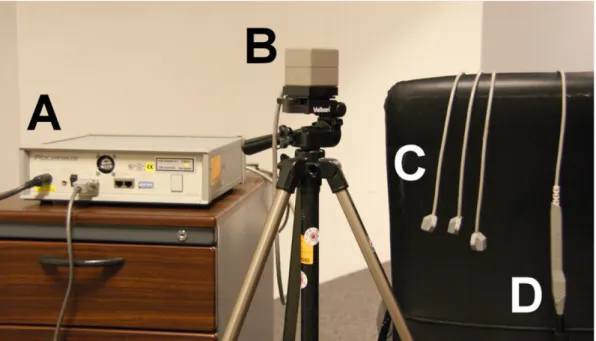
Figure 5. EEG recording apparatus ...13

Figure 6. 3D digitizer system ...14

Figure 7. Channel location recording by 3D digitizer system ...15

Figure 8. The artifacts contaminated epoch and channel from the subject S02 ...19

Figure 9. The relationship between the channel and component activities ....20

Figure 10: The scalp maps of 30 ICs derived from the event-related lane-departure response epochs from a single subject...23

Figure 11. The IC clusters of central, parietal, occipital, left and right somatomotor components ...24

Figure 12. The baseline power spectra of projected channel activities in occipital area before and after the EEG data normalization...26

Figure 13. Schematic overview of baseline power spectral analysis...28

Figure 14. The box-plot of alertness RT for 11 subjects before and after RT normalization ...31

Figure 15. RT distributions of the current, next, and 2’nd next trials under alert, drowsiness with and without warning conditions...33

Figure 16. The grand mean of baseline power spectra of the occipital area in current, next and 2’nd next trials across the alert, drowsy with and without warning conditions...35 Figure 17. The box-plots of the alpha and theta power of current, next and

2’nd next trails across alert, with and without warning conditions ..36 Figure 18. The grand mean of baseline power spectra of the central, left

and right somatomotor and the parietal areas in current, next and 2’nd next trials across the alert, drowsy with and without warning conditions...37 Figure 19. The grand mean of baseline power spectra of the occipital area

in current and next trials across short, medium and long RT

groups...40 Figure 20. The box-plots of the alpha and theta power of current and next

trials under alert, with and without warning conditions across

three different RT groups ...42 Figure 21. The mean response-locked event related alpha- and theta-band

power perturbations of alert, drowsy with and without warning

trials in the occipital area ...43 Figure 22. The examples of three-trial and two-trial selection...59

List of tables

Table 1. The mean and standard deviation (S.D.) of alertness RT. ...17 Table 2. The epoch and channel number of each subject...18 Table 3. The summary of RTs for current, next and 2’nd next trials under

alert, drowsy with and without waning conditions. ...32 Table 4. The alpha and theta power of curent, next and 2’nd net trails under

alert, drowsy with and without waning conditions. ...35 Table 5. Summary of spectral characteristics of three RT groups ...39 Table 6. Summary of effects of warning on averaged alpha- and theta-band

1.

Introduction

1.1.

The importance of drowsiness detection

Studies reported that fatigue, which, in turn, caused drivers inattention or drowsiness, was the major risk factor for serious injury and death in car accidents [1-4] National Sleep Foundation (NSF) reported that 60% of drivers had felt drowsy during driving, and 37% of the drivers had actually fallen asleep. The National Highway Traffic Safety Administration (NHTSA) also reported that at least 100,000 police-reported crashes were directly caused by drowsy driving in 2006 and leaded to 1,500 deaths, 71,000 injuries and $12.5 billion in monetary losses (National Sleep Foundation 2007 State of the States

Report on Drowsy Driving). Therefore, to early detect the drivers’ drowsiness

and to help to keep the drivers’ alertness for avoiding the car accidents that caused by drowsiness are important to protect living safeties of people.

Drowsiness detection changes of the subject’s alertness have been widely investigated by different measurements [5, 6] including the monitoring subject’s behavior and image based techniques and physiological signal-based system. The advantage and limitation of these methods were described in the following paragraphs.

1.2.

The behavioral monitoring

Previous studies had shown that subject’s response performance is deteriorated along with the drowsiness. The response performances were

of drivers’ moving handle wheel [11, 12]. The limitation of behavioral monitory system is highly depended on driving behavior, experiences, road conditions, and all other environmental variables. Therefore, it is difficult to be generalized for regular use. However, it can be used as an auxiliary method in the image-based techniques or physiological signal based system to define or verify the subject’s alertness according to the car deviation from the cruising lane and the response time (RT) to specific driving conditions. Such methods have difficulties to apply in the real driving since it is easily affect by the sounded environment and it is still unclear to what extend the behavioral responses can fully reflect the real cognitive status. But, previous have showed that behavioral performance is opposite correlated with the driver’s alertness. Specifically, the subject’s response performances, which index by response time, are decreased along with the increases of drivers’ drowsiness [13, 14].

1.3.

The image-based technique

The image-based technique uses the video camera to record the eye gaze position, eye closure or the head position [15] to derive the duration of eye gaze fixation and the eye closure or frequency of eye movement, eye blinking [16-18] or head movement [19] for correlating the subject’s drowsiness level. The advantage of the image based detecting system is nearly no need for preparation before the experiment, which is contrast to the long preparation time in the EEG based monitoring system. However, the quality of recorded image is easily influenced by the environment [20], with which is necessary for the camera needed to interact. Furthermore, it is difficult to get enough space to mount two cameras inside the cabin and without blocking the driver’s

viewing angle and therefore reducing the driver’s visual field [21]. Second, the response time for detecting driver’s drowsiness was too long to feedback to the driver in real time [22].

1.4.

The physiological signal based system

Abundance of studies used the physiological signals, including the electrocardiograph (ECG), electro-oculograph (EOG), or electroencephalograph (EEG), to monitor the subject’s alertness. The heart rate or heart rate variability [23] which derived from the ECG signals has been known easily affected by the subject’s psychological and physiological conditions and therefore the ECG signals is not a good index for monitoring the driver’s alertness. Some laboratories tried to use the EOG signals to index the driver’s alertness. For example, they found that the rate of eye blinking [24] was declined along with the decreases of subject’s alertness. However, the time window for analyzing the EOG signals to assess the driver’s drowsiness was around 240 sec, which is too long to use in the drowsiness warning system in the real driving. Hence, the EEG signals se the limitation of long average windows to detect drowsiness. Therefore, EEG remains the most popular modality and the better methods used to monitor drowsiness state in real-time.

1.5.

Drowsiness related EEG features

Studies had shown that the brain activities are changed with the subject’s drowsiness level, especially the neural activities generated from the occipital

(4-7 Hz, [27-30]) were incremented along with the decreases of subject’s performances. The similar brain dynamic changes are also observed in the simulated driving condition. Lin et al. [31] reported that the power of occipital alpha band was linearly increased from alertness to mild drowsy and then the alpha power was maintain at the same level or slightly decreased from mild drowsiness. In addition, the occipital theta power was also found increased monotonically from alert to deep drowsy. The above results suggested that occipital alpha and theta bands would be as good EEG features for indexing the subject’s drowsiness.

1.6.

Effects of warning signals under drowsy

condition

Many studies had tried to use the warning signals to keep driver’s attention [32-34]. They delivered the warning stimulations mainly via the acoustic [35], visual [36] or vibrated stimuli [37, 38]. Furthermore, some studies also tried to simultaneously present the warning signals via the multiple modalities [39]. Belz et al. compared the above warning modalities in terms of the reaction time (RT) to each warning modality [40]. Results showed that subject responded to the visual alarms with the longest RT since the driver needed to pay attention to the road condition and the dashboard. Therefore, the visual alarms are adequate as the warning stimulus. The multiple-warning modality significantly improved the driver’s performances by accelerating the RT. The acoustic stimuli also greatly improve the driver’s RT while the characteristics of the warning signal would significantly affect the results of the warning.

The warning sounds could be classified into two types, the conventional warning signals and the auditory icon [41, 42]. The conventional sounds were generated with specific acoustic parameters, such as pure tones, bells, buzzers and sirens. The auditory icons were sounds with specific stereotypical meanings defined by the objects or actions. For example, the horn or tire-skid, imply the emergency braking or car accident. Graham assessed these two types of sounds by measuring the driver’s RT [41]. Though results revealed that auditory icons significantly reduced the RT compared to the responses to conventional warnings, the auditory icons are also known to cause the driver to respond alarms improperly and increasing the risk of car accidents. Therefore, the auditory icons would not be safe to widely apply on real driving. Our previous studies evaluated effects of the spectrum and delivering patterns of conventional sounds on keeping the driver’s attention [43]. We delivered two types of sound patterns (continuous tone and tone bursts) and each pattern was tested by three different carrier frequencies (500, 1750, and 3000 Hz). Results showed that tone bursts with the carrier frequencies at 1750 Hz significantly improved the driver’s performances and without side effects on driver’s driving behavior.

1.7.

Aims of this study

Effects of alarms on maintaining driver’s attention and alertness were assessed in terms of the behavioral responses. To what extent the behavioral performance can reflect on the subject’s cognitive status and neural activities remains unclear. Some studies have observed that the behavioral performance might not be sufficient to fully mirror the real cognitive state

though lots of results showed that the behavioral performance was highly correlated with the brain dynamic [44, 45].

The first aim of this study was to determine the effects of the auditory alarm on the brain dynamics, which explored by the EEG. The second aim of this study was tried to elucidate whether the brain activities could fully mirror the behavioral indexes.

2.

Methods

2.1.

Subjects

Eleven subjects (ages from 18-29 years, 10 males and 1 female) were paid to participate in this experiment. They didn’t have psychological and neurological diseases. They had normal or corrected-to-normal vision and normal hearing. All subjects had no sleep disorders and they were required to go to sleep before the 1:00 AM at the night before the experiment. The subject had a lunch before the experiment and the experiment started around 2:30 PM since previous studies suggested that the drowsiness easily occurs from late night to early morning and during the early afternoon, especially after the lunch. All the experimental procedures was explained to the subjects in details and required by the instructions (Appendix I). Subjects were required to sign the research consent before the experiment. After the placement of electrodes, subjects were asked to practice to keep the car on the center of the cruising lane by maneuvering the car with the steering wheel at least for 5 min until they had expected performance. After the end of the experiment, every subject was

required to fill a questionnaire (Appendix II). Each subject had to complete the experiment for at least 60 min.

2.2.

Experimental apparatus

2.2.1. Virtual reality driving simulation environment

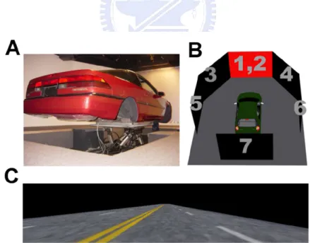
The driving simulated environment was composed of the virtual reality (VR) scenes and the driving simulator. A real car without engine and other non-necessary parts was mounted on a 6-degree of freedom motion platform (Figure 1A). All the VR based driving simulated environment was built up in our previous studies [46, 47]. The VR-based high way scenes were generated from seven personal computers which synchronized by the internet connection and then were projected to seven screens via seven projectors (Figure 1B).

Figure 1. The virtual reality environment. A: A real car without the engine and other unnecessary parts were mounted on the motion platform. B: The schematic picture shows the 360°-surrounded virtual reality scenes which projected from seven projectors. C: The picture shows the four-lane highway scene which used in the event-related lane-departure task.

2.3.

Experimental paradigm

2.3.1. The event-related lane-departure task

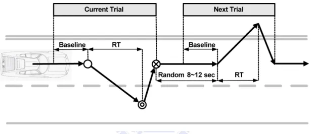
The event-related lane-departure task [48] was designed to index the driver’s drowsiness level. The event-related lane-departure task was a 4-lane high way scene (Figure 1C). The digitized VR scene was divided into 233 points and the width of the individual lane and car were 60 and 32 points respectively. The refresh rate of the VR scene was 60 Hz, which can properly emulate a car driving at a fixed speed of 100 km/hr on the highway. All scenes were updated according to the displacement of the car and the subject’s wheel handling. The car was randomly drifted away from the center of the cruising lane, which was controlled and triggered from the WTK program, to mimic the consequences of a non-ideal road surface [49-51]. The inter-deviation intervals were varied from 8 to 12 sec and the car was deviated either left or right with the equal chance. This task required subjects to compensate the drifting by manipulating the steering to keep the car on the center of third cruising lane (from left to right counted). During the experiment, subjects were instructed to continuously perform the task as best as they could even if they began to feel drowsy. No intervention was made when the subjects was occasionally fell asleep and stopped responding. After such non-responsive periods subjects resumed task performance without experimenter intervention. The onset of each deviation and the subject’s response time were recorded at the rate of 60 times per second via a synchronous pulse marker train that was recorded in parallel by the EEG acquisition system for the further off-line analysis. Figure 2 illustrates the experimental paradigm and the temporal profile of a typical deviation event in the event-related lane-departure task. Though the task is a

60- to 90-min continuous experiment, it contained the single trials in this task. Each complete single trial started from the 3 second before the car drifting to the subject’s response offset. The baseline period of individual trials was the duration of 3 sec before the deviation onset, and the response time (RT) was calculated the period from the deviation onset to the subject responded to the deviates by manipulating the wheel handling.

Figure 2. A bird’s eye view of the event-related lane-departure event. The car cruises with a fixed velocity of 100 km/hr on the VR-based highway scene and every 8-12 sec the car is randomly drifted either to the left or to the right from the cruising position to mimic the non-ideal road surface. Subjects are instructed to steer the vehicle back to the center of the cruising lane as quickly as possible. The solid black arrows mean the virtual car trajectory. The open circle is the deviation onset. The double circle is the response onset. The circle with cross is the response offset. The baseline is the duration from 3 sec before to the onset of car drifting. The response time (RT) is the time duration between the deviation onset and response onset. A completed trial is from 3 sec before the deviation onset to the response offset.

2.3.2. Warning criterion

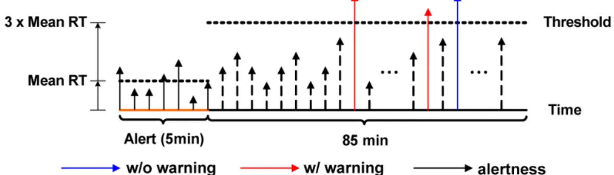
We used the 1 tone bursts with frequencies and intensities at 1,750 Hz and 68.5 (±1.5 dB) as the warning stimuli since our behavior studies had shown that the stimuli can effectively keep the driver’s alertness [43]. The background high way noise was 54 ±1.5 dB. The speaker was mounted on the back seat which is 90 cm apart from the subject. The first 5 min after the onset of the experiment, every subject was keep alert and the average RT was recorded and calculated as the criteria for delivering the warning signals. When the subject got drowsy and their RTs were longer than 3 times of the mean alert RT [31], the waning sound was delivered to the subjects randomly. Specifically, only half of drowsy trials, which the RTs were longer than 3 times of averaged RT under alert condition, were alarmed by the tone bursts (Figure 3). The response time and the EEG traces of those trials with warning (w/) and without warning (w/o) were extracted and compared for the offline analysis.

Figure 3. The schematic picture showed the criteria of delivering warning stimuli. The length of the arrows represents the response time of each single trial. Black solid arrows are those trials in the alert session. The threshold (dashed line) is set at the three times of mean alertness RT. Blue solid arrows are those trials with RTs longer than the threshold but without warning (w/o trials). Red solid arrows those trials with RTs longer than the threshold with warning (w/ trials).

2.4.

Data acquisition

2.4.1. Behavior data

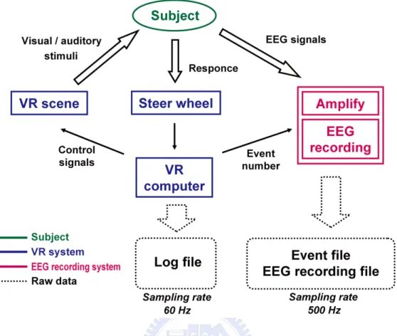
The sensor on the steer wheel was a variable resister and the output range was ±10 V depending on the rotation angle. The analog voltage signals were digitized by the analog to digital convert with the 12 bit vertical resolution and then stored into the personal computer for the offline analysis. The onset of car drifting and the subject’s responses, including the response onset and offset, were recorded at the rate of 60 times per second and saved as log file and recorded in parallel by the EEG acquisition system via a synchronous pulse marker train. Since the sampling rate of the EEG system was 500 Hz, the EEG system was easily to over sampled the same point, the log file was used as the look-up table for deleting the oversample data points. Figure 4 is the flowchart of the relationship among the VR scene EEG data acquisition system and behavioral data acquisition system.

Figure 4. Data acquisition flow chart. The flowchart illustrates the relationship among the VR scene EEG data acquisition system and behavioral data acquisition system.

2.4.2. EEG data

2.4.2.1. Channel location measurement

A sintered Ag/AgCl electrode cap with 30 channels (plus 2 references) was mounted on the subject’s head for recording the brain activities from the skull. All channels were displaced according to the modified International 10 - 20 system (Figure 5A and 5B). The actual location of each channel were redigitized by the 3D digitizer (Fastrak®, Polhemus, Figure 6) for rebuild individual subject’s head model by the mathematical algorithms [52] for localizing the sources of brain activities.

Figure 5. EEG recording apparatus. A: The schematic picture shows the channel locations of 30-channel recording system. B: A photomicrograph shows the real electrode cap placed on a head model. C: A photomicrograph shows the EEG amplifier used in the experiment. Our caps had 30 channels. Note the channel locations of each subject depended on the 3D measurement results.

2.4.2.2. Amplify the EEG signals

To minimize the contact impedance of each electrode is necessary for reducing the external noise coupling and increasing signal to noise ratio during the EEG recording. For minimizing the contact impedance, the conductive gel (Quik-GelTM_{, Compumedics NeuroMedical Supplies}TM_{) was carefully filled}

into each channel. Before data collection, the contact impedance of the EEG electrodes was less than 10 kΩ. The EEG activities were recorded and amplified by the Neural Scan Express System (NuAmps, Compumedics Ltd., VIC, Australia, Figure 5C). The input range of the EEG amplify is ±130 mV and the sampling rate and the vertical resolution are 500 Hz and 16-bit respectively.

Figure 6. 3D digitizer system. The 3D digitizer (Fastrak®, Polhemus) was used to measure 3D positions. A: The System Electronics Unit (SEU) can supply power and connect to other parts and computer. B: the transmitter is the device which produced the electro-magnetic field and is the reference for the position and orientation measurements of the receivers. C: The receivers are the smaller device whose position and orientation was measured relative to the transmitter. D: The stylus is a pen shaped device with a receiver coil assembly built inside and a push button switch mounted on the handle to effect data output.

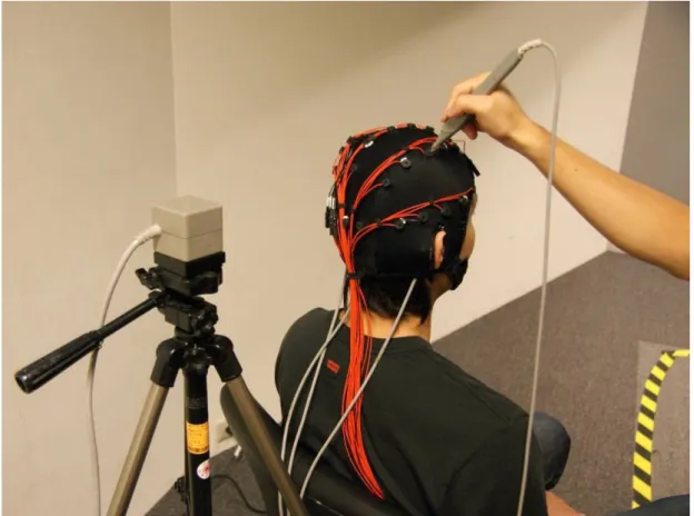
Figure 7. Channel location recording by 3D digitizer system. A photograph shows the 3D digitizer system for digitizing and recording the real locations of each channel in individual subject. The processing is described as following. While we measured the 3D position of the channels, we mounted the transmitter behind the subject and put the 3 receivers under the Oz, T3, and T4 channel inside the electrode cap. The transmitter should far from the metallic surface and located in close proximity to the receivers. Beside, we routed the transmitter cable separate from the receiver cables in order to avoid possible noise problems. After these setups, we used the stylus to point out each channels and recorded the 3D channel locations.

2.5.

Data analysis

2.5.1. Behavior data processing

2.5.1.1. Removing incomplete trials

A total of 4073 trials were recorded from 11 subjects and 521 incomplete trials were removed before the further analysis. The criteria marked as the incomplete trials were determined by the following rules. First, events recorded were incomplete. For example, each trial was recorded the occurrences of three events (deviation onset, response onset and response offset), and those missed one of the three event were first removed from the total trials. Second, those trails show the subjects didn’t follow the experimental instruction in terms of the trajectories were removed. Specifically, once the subjects didn’t follow the experimental instructions, the position of the deviation onset was located outside the third lane or the sawing line instead of the straight line was showed in the baseline line trajectories. Third, those trials with the RT less than 0.4 sec or longer than 9 sec were removed. The RTs shorter than 0.4 sec were due to subjects adjust the steering wheel but not responses to the car drifting. The RTs longer than 9 sec were due to the subjects were fall asleep and these trials were not defined as the drowsy trials.

2.5.1.2. RT normalization

Since the data were pooled across 11 subjects for the limited recording time from each single subject, we first needed to normalize the response time for reducing the inter-subject variation. The RTs of each subject were divided

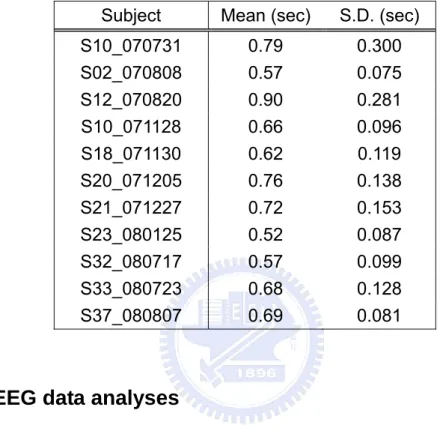
by their individual mean RT. The mean RTs were varied from 0.52 to 0.9 sec across 11 subjects (Table 1).

Table 1. The mean and standard deviation (S.D.) of alertness RT.

Subject Mean (sec) S.D. (sec) S10_070731 0.79 0.300 S02_070808 0.57 0.075 S12_070820 0.90 0.281 S10_071128 0.66 0.096 S18_071130 0.62 0.119 S20_071205 0.76 0.138 S21_071227 0.72 0.153 S23_080125 0.52 0.087 S32_080717 0.57 0.099 S33_080723 0.68 0.128 S37_080807 0.69 0.081

2.5.2. EEG data analyses

2.5.2.1. Preprocessing and extracting epoch

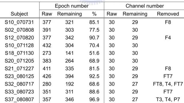
The raw EEG signals were first filtered by a low pass and a high pass filtering with the frequencies at 50 Hz and 0.5 HZ respectively to remove the 60Hz line noise, high-frequency artifacts and the low frequency drifting. The filtered signals were down-sampled into the 250 Hz sampling rate for the simplicity of data processing. EEG epochs were extracted from the continuous EEG signals and the duration of each epoch was 45 sec, 15 sec preceding and 30 sec following the deviation onset of each trial. A total of 4058 epochs were extracted and the number of epoch was varied from 273 to 432 across 11 subjects (Table 2).

2.5.2.2. Artifacts rejection

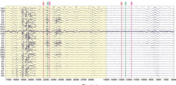
The extracted epochs were further examined and manually removed those epochs contaminated with muscle activities, body movements and bad contact channels. Figure 8 shows the example of the rejected epochs from a typical subject (S02). The EMG artifacts embedded in the epoch during the periods from 18 to 21sec and 23 to 24 sec was first selected and marked by yellow background and then was removed from the EEG signals. The FCz channel showed in the Figure 8 was identified as the bad contacted channel and was removed from the EEG signals.

A total of 3253 epochs were submitted to the further analysis after the artifact rejection and the number of epoch was varied from 11 subjects. (Table 2)

Table 2. The epoch and channel number of each subject.

Epoch number Channel number

Subject Raw Remaining % Raw Remaining Removed S10_070731 377 321 85.1 30 29 F8 S02_070808 391 303 77.5 30 30 S12_070820 377 342 90.7 30 29 F4 S10_071128 432 304 70.4 30 30 S18_071130 273 141 51.6 30 30 S20_071205 383 264 68.9 30 30 S21_071227 411 335 81.5 30 29 F8 S23_080125 426 394 92.5 30 29 FT7 S32_080717 280 192 68.6 30 27 FT8, T4, FT7 S33_080723 351 311 88.6 30 29 FT7 S37_080807 357 346 96.9 30 27 T3, T4, P7

Figure 8. The picture shows the artifacts contaminated epoch and channel from the subject S02. Two epochs are shown in the figure, and the two epochs were separated by a blue dash line. The red (event number 251), green (event number 253), and pink (event number 254) lines represent the deviation onset, response onset and response offset respectively. Note the artifacts are embedded in the first epoch with the periods at 18-21 and 23-24 sec. The epoch with artifacts is indentified and marked as yellow background and is removed from the extracted epochs. The channel (FCz) contaminated with noise is also indentified and rejected manually from the extracted epochs.

2.5.2.3. Independent component analysis (ICA)

Because of the volume conduction of the skull and scalp tissue [52], the signal recorded from individual electrode is easily mixed with signals generated from other brain regions or which are not located at the position around the electrode or other sources outside of our brain, such as the eye blinking and the eye movement (Figure 9). For indentifying the more corrected brain sources from the mixing EEG signals and removing the unrelated signals to obtain the pure neural activities we applied the ICA algorithm (the runica function of the EEGLAB toolbox) on the EEG signals to separate these mixing

The independent component analysis has extensively applied on blind source separation problem [53-55]. The ICA theorem had four basic assumptions. First, the source signals (neuron activities, noises, or artifacts) were independent to each other and the correlation between each two sources was zero or close to zero. Second, the propagation delay from sources to sensors was negligible. Third, the sources were analog and the possibility density function (p.d.f.) was not the gradient of a linguistic sigmoid. Fourth, the number of sources was the same as the number of sensors (channel signals) [56].

Figure 9. The schematic picture shows the relationship between the channel and component activities. The channel signals (channel A, B) ideally were a linear combination of many independent sources (component 1, 2) produced by the weight matrix W. By the ICA analysis, we could get the values of matrix W and separate the each component signals from the mixing channel data.

Due to the characteristic of the independent neuron activities in human brain, the EEG model could satisfied the 1’st, 2’nd, and 3’rd assumption. Although no one knows how many sources can the brain be activated and classified, based on the reports of past studies [57, 58], the ICA algorithm is still a good solution to solve the EEG source separation, identification, and localization. The ICA mathematical description was as follows.

AS

X

=

U

=

WX

[

]

T (t) (t) (t)

s

s

s

1 2

L

m

=

S

[

]

T (t) (t) (t)

x

x

x

1 2

L

n

=

X

[

]

T (t) (t) (t)

u

u

u

1 2

L

n

=

U

⎥

⎥

⎥

⎥

⎦

⎤

⎢

⎢

⎢

⎢

⎣

⎡

=

nm

a

a

a

a

a

a

n m

L

L

M

O

M

M

O

L

1 21 1 12 11

A

⎥

⎥

⎥

⎥

⎦

⎤

⎢

⎢

⎢

⎢

⎣

⎡

=

nn n n

w

w

w

w

w

w

L

L

M

O

M

M

O

L

1 21 1 12 11

W

S represents the real neuron activities (or artifacts) that generate from

total m (we did not know and too many) sources. The X is the n (channel number) channel signals that we recorded. The matrix A is the real weight that is used to transform the source signals into the channel activities. The matrix

W and the U, which represented the n (component number) main components

can be obtained by the ICA analysis. Once the channel number n is close to the real number of sources, m, the components U obtained by ICA algorithm, will be very close to the real source activities, S. EEG signals were separately

2.5.2.4. Component selection

The scalp map, the dipole location and the power spectrum of each component from individual subject were generated by using the function

topoplot and pop_dipfit_gridsearch of EEGLAB toolbox. The scalp maps of

each component represented the relative weight to compose from the channels (Figure 10). The scalp maps were also revealed the spreading of the component topography.

The separated components from each subject were further selected according to the scalp map, dipole location of each component and the characteristics of the power spectrum and only those scalp maps represented the sources generated from the occipital, somatomotor, central and frontal areas were submitted for the further analysis. Figure 10 shows the example of the 30 isolated component scalp map from the single subject (S02). Only the component 3, 4, 5, 7, 8, and 10 were selected for the further analyzed.

Figure 10: The scalp maps of 30 ICs derived from the event-related lane-departure response epochs from a single subject (S02). The noise components including the IC 1, 2, 6, 9, and 11-30 were excluded and the activities of IC 3-5, 7, 8 and10 were selected (circled) for further analyses.

2.5.2.5. component clustering

The selected components across 11 subjects were further classified manually into five clusters based the scalp maps, dipole locations and the baseline power spectra. EEG signals of the five main component clusters represented activities recorded from the central, left somatomotor, right somatomotor, parietal, and occipital areas (Figure 11). Activities of the central left-somatomotor, right-somatomotor, parietal and occipital components which are known to highly correlate with the drowsiness or motor responses were selected for the following studies.

Figure 11. Pictures shows the IC clusters of central, parietal, occipital, left and right somatomotor components. The left panel shows the individual scalp maps of included in the corresponded component clusters. The subject index and component number was marked on the top of each scalp map, and the larger scalp maps are the mean of the scalp map averaged from the individual ICs. The right panels were the dipole locations of each single component across 11 subjects.

2.5.2.6. Component activities back projected to channel activities

According to the ICA algorithm, the signal excursion of each component only represented the relative amplitude of the brain activities generated from the specific brain area. In order to transform the amplitude of component activities into the real scale, activities of the central, left-somatomotor, right-somatomotor, parietal, and occipital components were need to back projected to Cz, Cp3, Cp4, Pz, and Oz respectively.

2.5.2.7. EEG signal normalization

Since the amplitude of EEG signals was varied across different sessions and subjects and such differences would lead to the differences observed in the EEG power spectra, the back projected channel activities were normalized by dividing the EEG signals to the standard deviation (SD) of the signal distribution before advanced analysis.

Figure 12 showed the baseline power spectrum of projected channel activities in occipital area cross 11 subjects before (A) and after (B) EEG data normalization. The results showed that baseline power spectrum after normalization had smaller power differences than before normalization.

Figure 12. The baseline power spectra of projected channel activities in occipital area before (A) and after (B) the EEG data normalization.

2.5.3. Data grouping

The normalized behavior and EEG data of each single subject were selected and grouped together according to the following procedures.

First, trials recorded in the alert session were selected and classified as the alert trials. Trials with normalized RT more than 3 times of mean RT under alertness were selected and classified as drowsiness trials.

Second, drowsiness trials with or without warnings, including the current, next and 2’nd next trials, were selected and separately grouped together for the next step processing. The details of the data selection were included in the Appendix III.

2.6.

Time-frequency analysis

Previous studies suggested that drowsy dependant EEG dynamics can be observed from two different aspects, the tonic and phasic changes [59, 60] and both aspects were processed by frequency analysis. Specifically, tonic changes referred to changes of baseline power spectra associated with changes in cognitive state (e.g., arousal or drowsiness) while phasic changes referred to those power changes triggered by specific events, such as the behavioral responses or warning stimuli. In this study, we first used the time-frequency analysis [61] to transform the grouped data trials into time–frequency data matrices and derived the baseline spectra and the event-related power perturbation to reveal effects of warning on tonic and phasic changes. The flow chart of time-frequency analysis shows in Figure 13.

Figure 13. Schematic overview of baseline power spectral analysis. The moving-window discrete wavelet transforms (DWTs) was used to transform the time domain EEG activities into spectrotemporal activations. The baseline spectrum and the event-related power perturbation were derived from the time-frequency data matrices.

2.6.1. Baseline power spectral analysis

The normalized EEG activities were transformed into a (400 latencies by 193 frequencies) time-frequency data matrix using a moving-window average of discrete wavelet transforms (DWTs, timef function from EEGLAB, [60]). DWTs were computed for 1.5-sec moving windows centered at 400 evenly spaced latencies from 15 sec before to 30 sec after the deviation onset using a data-window length of 375 points (1.5 sec), zero-padded to 3000 points. Log power spectra were estimated at 193 evenly-spaced frequencies from 2 Hz to 50 Hz, and the log mean power spectral baseline was the averaged power change during the pre-deviation period (-3-0 sec).

2.6.2. Event-related spectrum perturbation (ERSP)

For assessing the sustainable effects of warning sounds, we extracted the long epochs (-15-130 sec) to estimate the changes of ERSPs. The activities of long epochs were transformed into a (725 latencies by 263 frequencies) time-frequency data matrix using a moving-window average of discrete wavelet transforms (DWTs, timef function from EEGLAB, [60]). DWTs were computed for 4.0-sec moving windows centered at 725 evenly spaced latencies from 15 sec before to 130 sec after the deviation onset using a data-window length of 725 points (4.0 sec), zero-padded to 2900 points. Log power spectra were estimated at 263 evenly-spaced frequencies from 0.75 Hz to 49.875 Hz. The temporal profile of the alpha (8-12 Hz) and theta (4-7 Hz) band power changes were extracted and averaged from the time-frequency data matrix for the advanced comparison.

2.6.3. Statistics

The Kolmogorov-Smirnov test (kstest, Matlab statistical toolbox, Mathworks) was used to assess whether the behavior RTs and EEG power were normally distributed (with zero mean and unit variance). Since tested results showed the behavior RT and EEG power were not normally distributed, three non-parametric statistic tests were used for the following statistical analysis. The Kruskal-Wallis one-way analysis (kruskalwallis, Matlab statistical toolbox, Mathworks) were used to assess the differences of inter-subjects’ normalized RTs across 11 subjects. The Wilcoxon rank sum test (ranksum, Matlab statistical toolbox, Mathworks) was used to evaluate the warning effect on RTs. Third, the permutation-based statistics [62-64], or called bootstrapping (statcond, EEGLAB toolbox, UCSD) was used to test the significance of the power changes of specific frequency bins induced by drowsiness or warning sounds. We boosted the sample size from about 200 trial number to 5000 by the bootstrapping methods.

3.

Results

3.1.

Behavioral performance

Figure 14 showed the alertness RT distribution of 11 subjects before and after behavior data normalization. Results showed that alertness RTs before normalization had significant differences across 11 subjects by the Kruskal-Wallis test (p<0.001) and such inter-subject difference was not significant after normalization (p=0.53).

Figure 14. The box-plot of alertness RT for 11 subjects before (A) and after (B) RT normalization. The red lines represent the medians of the alertness RT distribution of each subject. The top and bottom of the blue box are the third and first quartile. The dash lines represent the region of RT between the maximum and minimum after outlier removal. The red crosses mark the outliers. Note the alertness RT distribution has significant difference (p<0.001) across 11 subjects before normalization and such difference was not significant after normalization (p=0.53).

3.1.1. Effects of warning sounds

A total of 1232 trails were included and presented in these results. Three conditions were included in these trials (alertness, drowsiness with warning and drowsiness without warnings) and all individual conditions contained the current, next and second next trials. Table 3 shows the number of trials, medians and quartiles of normalized RTs across these three conditions under different groups of trials.

Figure 15 shows the cumulated normalized RT of current, next and 2’nd next across the alertness, drowsiness with warning and without warnings.

Figure 15A shows the cumulated distribution of the RTs of current, next and 2’nd next trials under alertness and drowsiness with and without warning. The RT distributions were different among the alert, drowsy with and without warning trials. RTs of all alertness trials were shorter than 3 normalized unit (nu) while RTs of all drowsy trials were longer than 3 nu. The warning sound significantly accelerated the RT. The cumulated curves of 50% trials with warning and without warning are statistically different (p <0.001, two sample KS test; Figure 15A left panel). The effect of warning on alerting the RT distribution was sustained to the next trials (p <0.01, Figure 15B). However, the effect of warning sound on RT was not significant in the 2’nd next trials (p =0.16, Figure 15C).

Table 3. The summary of RTs for current, next and 2’nd next trials under alert, drowsy with and without waning conditions.

Medium QD1 QD3 Trial number alertness 0.96 0.86 1.09 216 Current w/o warning 5.19 4.02 6.76 196 w/ warning 4.16 3.79 4.35 182 Next w/o warning 1.57 1.09 3.66 196 w/ warning 1.20 1.02 1.79 182 2’nd next w/o warning 1.30 1.05 2.31 132 w/ warning 1.20 1.07 1.73 128

Figure 15. A: Cumulative RT curves of the current, next, and 2’nd next trials under alert, drowsiness with and without warning conditions. The black, red and blue curves represent the RTs of alert, drowsy with and without warning trials, respectively. The black dash line at left panel marks the onset time of warning. B: The box-plots of the same data as in A. The horizontal lines inside the boxes represent the median. The top and bottom lines of the boxes are the third and first quartiles. The dash line marks the maximum and minimum after removing the outliers. Results showed that the RTs were significantly fast under the alertness condition in comparison with the drowsiness. Note: the drowsiness and warning sound can alter the distribution of RTs (drowsiness vs alertness: p<0.001; w/ vs w/o: p<0.001) and the effect of warning can sustain to the next trials (*: p<0.05, **: p<0.01, ***: p<0.001).

3.1.2. Effects of warning on brain activities

3.1.2.1. Occipital region

Since the occipital neural activity is known to highly correlate with drowsiness, we first assessed the effects of warning on altering occipital dynamics. Figure 16 shows the EEG baseline spectra of alertness (black curve), with (red curve) and without warning (blue curve) trials. Comparing with the alertness, the averaged baseline power spectra of the drowsy trials were significant higher at frequencies from 2 to27 Hz (p<0.01 Figure 16, left panel). From alert to drowsy, the alpha band power was elevated around 11 dB and the theta band power was increased around 5 dB (Table 4). No apparent differences of alpha- and theta-band power were found between trials with and without warning (Figure 17, alpha: p=0.46, theta: p=1.00).

The effect of warning on altering the occipital activities was revealed on the mean of baseline power spectra of next trails. Comparing with trails without warning, the amplitude of the averaged baseline power spectrum of warning trials was significant lower at frequencies from 2 to 9 Hz (Figure 16, middle panel). The theta- and alpha- brand power were significantly suppressed by the warning sounds (Table 4, alpha: 1.60 dB, p=0.01; theta: 1.74 db, p<0.001, by permutation-based statistics). Comparing with the alert trials, the grand mean power spectral baseline exhibited significant tonic power increases from 2 to 20 Hz in the trials with and without warning. The effects of warning did not extend to the 2’nd next trails. Though the tonic baseline power showed increases between alpha and theta bands in warning relative to without

warning trials (Figure 16, right panel), such differences were not statistically significant (alpha: p=0.07, theta: p=0.13, Figure 16).

Figure 16. The grand mean of baseline power spectra of the occipital area in current, next and 2’nd next trials across the alert (black), drowsy with (red) and without (blue) warning conditions. The green horizontal lines represent frequencies exhibiting significant (p<0.01) tonic spectral power increases (w/o warning minus w/ warning). The blue horizontal lines mark frequencies exhibiting significant (p<0.01) tonic spectral power increases (w/o warning minus alertness). The red horizontal lines show frequencies exhibiting significant (p<0.01) tonic spectral power increases (w/ warning minus alertness). The inset shows the averaged scalp map of occipital region across 11 subjects.

Table 4. The alpha and theta power of curent, next and 2’nd net trails under alert, drowsy with and without waning conditions.

Current Next 2’nd next

w/o warning 35.06 33.89 33.10 w/ warning 35.35 32.29 31.83 Alpha alertness 24.26 w/o warning 28.21 27.33 27.15 w/ warning 28.19 25.59 26.22 Thet a Alertness 23.22 Power (dB)

Figure 17. The box-plots of the alpha (A) and theta power (B) of current, next and 2’nd next trails across alert, with and without warning conditions. Panels as Figure 15B (*: p<0.05, **: p<0.01, ***: p<0.001).

3.1.2.2. Other brain areas

Figure 18 shows the averaged baseline power spectra of other brain area including the central, left and right somatomotor as well as parietal areas. Similar to the occipital area, the grand mean of power spectral baselines showed significant (p<0.01) tonic increases between 3-12 and 20-25 Hz in drowsy relative to alert trials for four brain areas (Figure 18). The tonic increases of baseline power spectra were not significant in warning relative to without warning trails for the central, left and right somatomotor and parietal areas.

Figure 18. The grand mean of baseline power spectra of the central (A), left (B) and right (C) somatomotor and the parietal (D) areas in current, next and 2’nd next trials across the alert (black), drowsy with (red) and without (blue) warning conditions. The insets on the right panel shows the averaged scalp maps of central, left and right somatomotor and parietal regions across 11 subjects. Panels as Figure 16A.

3.2.

The influence of drowsiness level on the outcome

of warning

The effect of warning on the RT distribution of next trials was mainly at those trials with RT from 1 to 4 nu (Figure 15). To determine to what extent the differential effects of warning signals would revealed on the brain dynamics, the current and next trials were all divided into three groups according to the distribution of next trials’ RTs (Figure 19, inset) and they were long (RT: 4-10 nu, A), medium (RT: 1-4 nu, B) and short RT (RT: 0-1 nu, C) groups. The averaged baseline power spectra of these three groups were calculated and compared as shows in the Figure 19.

The distribution of long and short RT groups were not significant different between the warning and without warning trials (long RT: p=0.4 and short: RT:

p=0.05, Table 5). For the medium RT group, the RTs were significant

accelerated in warning trials relative to those without warning trials (p<0.001, Table 5).

Figure 19 shows the differential effects of warning on the occipital neural activities for the current and next trials in long, medium and short RT groups. Both the current and next trials, the increased tonic baseline power was found in the drowsy relative to alert trials. Such differences between the alert and drowsy trials were not affected by the RTs. For the current trials, no apparent suppression on the increases of tonic baseline power spectra in the warning relative to those without warning trials and no clear differences were found among the three RT groups. In the next trials, the effects of warning on the tonic changes of the baseline power spectra were similar to those presented in

the Figure 16. For the medium RT groups, the grand average of power spectral baselines of next trials showed decreases between 2-9.5 Hz (Figure 19, B) in warning relative to without-warning trials, and for the medium RT groups the mean difference was significant (p<0.01) between 5-7 and 9.5-10.5 Hz (Figure 19, C). In the alpha and theta bands (8–12 Hz and 4–7 Hz) of both medium and short RT groups, mean tonic baseline power in warning trials was significantly (p<0.01) smaller than in without-warning trials (Figure 20, Table 6).

Table 5. Summary of spectral characteristics of three RT groups

Medium QD1 QD2 Mean SD A 1.22 1.16 1.32 1.25 0.11 B 0.96 0.90 1.03 0.97 0.08 C alertness 0.79 0.73 0.82 0.77 0.06 w/o warning 5.35 4.24 7.31 5.85 1.96 A w/ warning 4.21 3.90 4.49 4.20 0.52 w/o warning 5.06 3.93 6.61 5.41 1.80 B w/ warning 4.18 3.74 4.33 4.11 0.55 w/o warning 5.39 4.01 6.37 5.43 1.73 Current C w/ warning 4.00 3.62 4.24 4.04 0.53 w/o warning 5.30 4.25 6.20 5.46 1.40 A w/ warning 4.56 4.24 6.07 5.22 1.40 w/o warning 1.57 1.23 2.59 1.96 0.93 B w/ warning 1.20 1.10 1.42 1.35 0.45 w/o warning 0.93 0.86 1.00 0.91 0.09 Next C w/ warning 0.88 0.79 0.95 0.87 0.10

Figure 19. The grand mean of baseline power spectra of the occipital area in current and next trials across short, medium and long RT groups. The inset represents the sorted RT curves of next trial. All the trials are divided into long (A), medium (B), and short (C) RT groups. Panels as Figure 16.

Table 6. Summary of effects of warning on averaged alpha- and theta-band power of current and next trials across three RT groups. Current Next w/o warning 35.15 35.18 w/ warning 34.85 35.59 A alertness 24.16 w/o warning 35.20 33.77 w/ warning 35.67 31.34 B alertness 24.22 w/o warning 34.54 32.55 w/ warning 34.76 28.94 Alph a C alertness 24.46 w/o warning 27.75 28.04 w/ warning 27.83 27.66 A alertness 22.97 w/o warning 28.46 27.49 w/ warning 28.34 25.13 B alertness 23.35 w/o warning 27.83 25.85 w/ warning 28.09 24.02 Thet a C alertness 23.04 Power (dB)

Figure 20. The box-plots of the alpha (A) and theta power (B) of current and next trials under alert, with and without warning conditions across three different RT groups. Panels as Figure 16 (*: p<0.05, **: p<0.01, ***: p<0.001).

3.3.

Alpha and theta bands perturbation

Figure 21 shows the power perturbations of alpha and theta band in with- (blue line), and without- warning (red line), as well as the alertness (black line). Before response onset, alpha- and theta-band power in drowsiness trails including the warning and without warning trials were 11.5 (alpha) and 5 dB (theta) higher than in the alertness trials. The alpha- and theta-band power of all drowsy trials, including the warning and without warning trails, showed brief decrease from 38 to 28 dB (alpha) and from 30.5 to 25.5 dB (theta) around the response onset. Comparing with the trials without warning, the event related

alpha band power was significant decreased in the warning trails mainly at 5-10 sec after the response onset. The event related theta band power of the warning trials was significantly lower at 5-35 sec after the response onset than in the trials without warning.

Figure 21. The mean response-locked event related alpha- (upper panel) and theta-band (lower panel) power perturbations of alert (black traces), drowsy with (red traces) and without (blue traces) warning trials in the occipital area. The green horizontal lines represent frequencies exhibiting significant (p<0.01) phasic spectral power decreases (w/o warning minus w/ warning). The inset shows the averaged scalp map of occipital region across 11 subjects.

4.

Discussion：

Aims of this study are to assess the effect of warning on behavioral performance and brain dynamics and to determine the sustainable duration of warning in terms of behavioral responses and neural activities. Results showed that the warning sounds can accelerated the responses to the car drifting and suppress the tonic and phasic power increases at the alpha and theta bands in the occipital area. Furthermore, the effects of the warning sounds on the behavior and brain activities could sustain to 12.6±2.7 and 10 sec respectively.

4.1.

Effects of drowsiness

Behavioral results showed that the sorted RT curves of drowsy trials, including the warning and without warning trials were all significantly departed from the sorted RT curves of alert current. This finding was consistent with previous studies suggested that the subjects’ behavioral performance was decreased along with changes of cognitive states from alert to drowsy [13]. The decremented behavioral performances could be assessed in terms of response time or driving trajectory [8, 9].

Our results also showed that the neural activities were also altered with the cognitive states. Specifically, both the tonic and phasic changes of the occipital area showed that the alpha and theta band power were increased in the drowsy relative alert trials. This finding was consistent with previous reports and our previous studies. For example, the tonic EEG power was higher on average in the drowsiness than in the alertness. In addition, the

increases of power in the low-theta frequencies near 4 Hz were highly correlated with the drowsiness [59, 65]. Huang et al. also reported the baseline spectra had tonic broad band power increases at the occipital area during periods of relatively poor driving performance and the prominent spectral changes were observed in alpha and theta bands [60]. Taken together, our results demonstrated that our experimental paradigm could successfully induced the drowsiness under driving condition in terms of behavioral performances and changes of brain rhythm at the occipital region. In addition, the warning sounds randomly delivered to the subjects did not affect the drowsiness induction during the experiment.

Except the occipital region, the power of the EEG spectra for central, left and right somatomotor and the parietal regions were increased around frequencies at 3-12 Hz (alpha and theta band) and 20-25 Hz (beta band). Results showed that the power increases at alpha, beta and theta bands associated with the drowsiness could be involved in large brain areas. Such phenomenon may due to the drowsy related brain dynamics was probably modulated by the independent modulators. The concept of the independent modulator hypothesized that the independent modulator could modulate the brain oscillations across several distinct cortical areas [66]. Effects of warning on altering the brain oscillations did not observed in other brain area. Such results suggested that those changes of brain dynamics were not due to the neural responses to the sounds.

4.2.

Effects of warnings

4.2.1. Behavior performance

Results showed that warning sounds improved the subject’s behavior performance by accelerating their RT. Specifically, the RTs of the current trials were significant shorten about 1.03 nu in the warning relative to without warning trials. The effects of warning on enhancing the behavioral performance also sustained to the next trails. Specifically, the warning could accelerate the RT about 0.37 nu faster than the RT of trials without warning. Lin et al. [43] showed that the mean RT of sessions with warning was significantly faster than that of sessions without warning. The mean RT was reduced by approximately 1.15 seconds. Several studies also reported that the warning sounds could help drivers to react promptly [67, 68] and reduce the probability of collision [68, 69].

Comparing with the RTs of alertness, the intervals between the onset of warning signals and the subject’s responses were still longer than the RTs of alert trials. The results implied that the warning signals could enhanced the behavioral performance but the subject’s conscious could be not as clear as the alert. The reasons may relate to the characteristics of warnings sound is not ideal or the single stimulus may not be enough to awake the subject. Study suggested that the characteristic of most powerful sounds to awake the drowsy driver is auditory icon, such as the horn or tire skid [40, 41]. In addition, auditory neuron has know easily adapt to the pure tone or pure tone burst [70]. In the auditory cortices, the majority of neurons are only responses to the complex sounds and only few neurons can respond to the pure tone or pure

tone burst [71]. Previous studies also suggested that warning signals delivered by the single modality may not sufficient to total awake the subjects and they suggested that warning signals delivered through the multimodalities, such as the combined the warning sounds and vibrations, could be a better methods to keep drivers’ alertness [72].

4.2.2. Brain dynamics altered by the warning sounds

The significantly inhibited the tonic increases of the mean baseline power were observed in the warning trials comparing with those trails without warning. The suppressed brain oscillations were mainly found at the theta and alpha bands, which are widely used as drowsiness related features [27]. The phasic decreases of the theta-band and alpha-band power were also observe in the ERSPs around the onset of the warning sounds and such the decreased of theta and alpha band power could sustain at least for around 10 sec. The findings suggested that that warning sounds would help drivers to reduce the drowsiness reflected on both behavioral performance and brain oscillations. This is the first study to show that the warning feedback could partially change the driver’s cognitive states. Consistent with the behavioral results, the neurophysiologic data also showed that the warning sounds couldn’t totally remove the driver’s drowsiness. In addition to the non-ideal characteristics and presentation modality of warning signals, such results may also relate to the effectiveness of warning feedback may decrease along with the increases of drowsiness. Comparing effects of the warning on altering the brain activities among three different RT groups, results suggested that the warning sounds could be effective when the normalized RTs was less than 4 nu, which indexed

block all the sensory inputs during the sleep [73]. It is still unclear that the thalamus gate would be digitally blocked or decreased the sensory inputs analogically from drowsy to sleep. According to our preliminary results, we speculated that the sensory inputs probably may be attenuated along with the degradation of the alertness. The control mechanisms of thalamus gate in details need to further assess in the future.

4.3.

Duration of the warning effects

The alpha- and theta bands showed different intervals of phasic power decreases. The duration of phasic alpha band decreases was around 10 sec, while the theta-band power decrease was around 35 sec. Such difference may due to the alpha band power have nonlinear and relative larger fluctuations in the theta band power during the transition from alert to drowsy. Studies showed the alpha activities increased and then started to decrease during wake-sleep transition [74-76]. Chuang et al. also reported that during mild drowsy period, the fluctuation of alpha activations was larger than theta and beta fluctuation [66]. Such alpha fluctuations could result from event-related desynchronization (ERD) and synchronization (ERS) of alpha activities [48, 60, 77] during the responses to the car deviation by manipulating the steering wheel.

The effects of warning sound can sustain for a short duration around 10 sec. This implies that the warning sounds could only transiently change the driver’s drowsiness. For the safety concerned, it is necessary to either combine with other feedback methods or to include the automatically driving system in the future to help the drowsy drivers to avoid the car crashes.