ELSEVIER Fuzzy Sets and Systems 86 (1997) 139 153
FOZZY
sets and systemsDesign of self-learning fuzzy sliding mode controllers based
on genetic algorithms
Sinn-Cheng Lin*, Yung-Yaw Chen
Lab. 202, Department of Electrical Engineering, National Taiwan University, Taipei, Taiwan, ROC Received March 1995; revised November 1995
Abstract
In this paper, genetic algorithms were applied to search a sub-optimal fuzzy rule-base for a fuzzy sliding mode controller. Two types of fuzzy sliding mode controllers based on genetic algorithms were proposed. The fitness functions were defined so that the controllers which can drive and keep the state on the user-defined sliding surface would be assigned a higher fitness value. The sliding surface plays a very important role in the design of a fuzzy sliding mode controller. It can dominate the dynamic behaviors of the control system as well as reduce the size of the fuzzy rule-base. In conventional fuzzy logic control, an increase in either input variables or the associated linguistic labels would lead to the exponential growth of the number of rules. The number of parameters or the equivalent length of strings used in the computations of genetic algorithms for a fuzzy logic controller are usually quite extensive. As a result, the considerable computation load prevents the use of genetic operations in the tuning of membership functions in a fuzzy rule-base. This paper shows that the number of rules in a fuzzy sliding mode controller is a linear function of the number of input variables. The computation load of the inference engine in a fuzzy sliding mode controller is thus smaller than that in a fuzzy logic controller. Moreover, the string length of parameters is shorter in a fuzzy sliding mode controller than in a fuzzy logic controller when the parameters are searched by genetic algorithms. The simulation results showed the efficiency of the proposed approach and demonstrated the applicability of the genetic algorithm in the fuzzy sliding mode controller design. © 1997 Elsevier Science B.V.
Keywords: Fuzzy control; Sliding mode; Fuzzy sliding mode; Genetic algorithms
1. Introduction
Recently, fuzzy logic c o n t r o l l e r s ( F L C s ) [8] b a s e d on a p p r o x i m a t e r e a s o n i n g [20] h a v e b e c o m e an e x t e n s i v e l y r e s e a r c h e d topic. A n u m b e r o f a p - p l i c a t i o n s h a v e c o n f i r m e d the c a p a b i l i t y o f F L C s [12, 16, 17]. In m o s t cases, the m o d e l s o f p l a n t s
* Corresponding author.
c a n n o t be easily derived. H o w e v e r , skilled o p e r - a t o r s c a n c o n t r o l the p l a n t s successfully b y s i m p l y f o l l o w i n g c e r t a i n linguistic s t a t e m e n t s , such as " I F condition A happens T H E N take action B ' . By i n c o r p o r a t i n g h u m a n e x p e r t i s e i n t o fuzzy I F T H E N rules, a linguistic F L C can be c o n s t r u c t e d to c o n t r o l c o m p l e x o r ill-defined systems. H o w e v e r , several w e l l - k n o w n difficulties still exist in F L C design: (1) F u z z y c o n t r o l rules a r e e x p e r i e n c e oriented. S u i t a b l e m e m b e r s h i p functions are usually 0165-0114/97/$17.00 q2' 1997 Elsevier Science B.V. All rights reserved
140 S.-C. Lin, K-K Chen / F u z ~ Sets and Systems 86 (1997) 139-153
obtained by time-consuming trial-and-error pro- cedures. (2) Characteristics of fuzzy control sys- tems cannot be pre-specified. (3) There is no criterion to obtain an optimal or at least sub- optimal FLC.
To overcome problems (1) and (2) discussed above, the fuzzy sliding mode control schemes have been extensively studied [3, 9-11, 13]. These ap- proaches are based on the fuzzy logic control and the sliding mode control [-19,4], and have the advantages of both. By introducing the concept of sliding mode to the F L C and fuzzifying the sliding surface, a fuzzy sliding mode controller (FSMC) has a "fuzzy" sliding surface. The control actions in a fuzzy sliding mode controller are smoother than those in a conventional sliding mode controller (SMC). As a result, chattering in an F S M C is smaller than that in an SMC. In FSMC, character- istics of the closed-loop control system can be spe- cified by a user-defined sliding surface. Moreover, establishing the control rules for F S M C is easier than that for conventional FLC. In this paper, we address the issue of using genetic algorithms (GAs) to solve problem (3). The goal is to find a sub- optimal rule-base as well as membership functions of FSMC. Such a sub-optimal F S M C can drive the system state to hit a pre-defined sliding surface as fast as possible, and keep the state sliding along the surface as close as possible.
Genetic algorithms were originally developed by Holland in 1962. The detailed principles, math- ematical frameworks and applications can be found in Goldberg's recent book [2]. The use of GAs for solving control problems was proposed in I-7]. In fuzzy control, GAs are always applied to search the string space, which is constructed by parameteriz- ing and encoding the rules or membership func- tions of an F L C into a binary string. Consequently, a sub-optimal F L C can be obtained [-5, 6]. How- ever, these strategies have a major drawback: when the number of input variables or linguistic labels increases, the number of fuzzy rules increases expo- nentially, which further leads to the exponential increase of the encoded string length. This paper will show that the number of rules in an F S M C is in proportion to the number of input variables so that the corresponding string length does not increase exponentially, but linearly.
This paper is organized as follows. Section 2 is a brief description of GAs. Section 3 presents the fuzzy sliding mode control method. Section 4 trans- forms the design problem of an F S M C to a se- arching problem that can be solved by GAs. In Section 5, simulation results are presented to verify the efficiency of the proposed approach. Con- clusions are given in Section 6.
2. Fundamentals of genetic algorithms
GAs are parallel and global search techniques which take the concepts from evolution theory and natural genetics. They emulate biological evolu- tions by means of genetic operations such as repro- duction, crossover and mutation. Usually, GAs are used as optimization techniques. Although there is no necessary and sufficient condition on the func- tions which are optimizable by GAs, it has been
shown that GAs perform well on multimodal func-
tions, i.e. functions which have multiple local opti- mums. Moreover, various studies have shown that whenever GAs failed to derive the optimal solution on a function, other known techniques failed as well [-2].
GAs work with a set of artificial elements (binary strings, e.g. 1 0 1 0 1 0 1 0), called a population. An individual (string) is referred to as a chromosome, and a single bit in the string is called a gene. GAs generate a new population (called offsprings) by applying the genetic operators to the chromosomes in the old population (called parents). Each iter- ation of genetic operations is referred to as a gen- eration. A fitness function, i.e. the function to be maximized, is used to evaluate the fitness of an individual. One of the important purposes of GAs is to reserve the better schemata, i.e. the patterns of certain genes, so that the offsprings may yield higher fitness than their parents. Consequently, the value of fitness function increases from generation to generation. In most of the GAs, mutation is a random-work mechanism to avoid the local opti- mum trapping problem. As a result, GAs always can find the global optimal solution.
The basic operations (i.e. reproduction, crossover and mutation) of a simple genetic algorithm (SGA) are described as follows.
S.-C. Lin, E-Y. Chen / Fuzzy Sets and Systems 86 (1997) 139 153 141
(1) Reproduction: The Darwinian "survival of
the fittest" is the underlying spirit of reproduction. First, a fitness value F is assigned to each individual string in a population. A higher F value indicates a better fit (or larger benefit). Next, the old indi- vidual strings are probabilistically selected and copied into a mating pool according to their fit- Uness value. The arrangement allows the strings with a higher fitness to have a greater probability of contributing a larger a m o u n t of offsprings in the new population.
(2) Crossover: Crossover provides a mechanism
for individual strings to exchange information via a probabilistic process. Once the reproduction op- erator is applied, the members in the mating pool are allowed to mate with one another. First, two parents are randomly selected from the mating pool. Then, a r a n d o m crossover point is picked up, on which the parents will exchange their genes. Finally, the parents' genetic codes are mixed by exchanging their codes following the crossover point. F o r example, consider two parent strings
1 0 1 0 1 0 1 0 0 I l l 1 1 0 0
The offsprings are in the following if the crossover point is 5:
1 0 1 0 1 1 0 0 0 1 1 1 1 0 1 0
This r a n d o m process provides a highly efficient method to search the string space to find a better solution.
(3) Mutation: At each iteration, every gene is
subject to a r a n d o m change with probability of the pre-assigned mutation rate. In the binary-coded case, a mutation operator changes a bit from 0 to 1 or vice versa. Overall, the mutation operation introduces new genes into the populations such that the trapping in local optimal points may be avoided.
The offsprings are generated from the parents until the size of the new population is equal to that of the old population, This evolution procedure progresses until the fitness reaches the desired specifications.
3. F u z z y sliding mode control
3.1. Some useful definitions of fuzzy logic control
The membership functions adopted in this paper are all Gaussian-type functions, i.e. # A ( X ) = e x p [ - ( ( x - m ) / o ' ) 2 ] , where m is the center of the membership function on which the membership grade IrA(m) = , and tr denotes the spread of the membership function. F o r notational simplicity, we express a fuzzy set A as A(m, a) here and hereafter. F o r example, the fuzzy set "Positive Medium" with m = 2 and a --- 0.7 is represented as PM(2, 0.7)
Definition 1. A fuzzy rule-base, R~=D~=IRt, is
a union of N fuzzy rules. Each rule R t in the fuzzy rule-base can be expressed as
Rt: I F xl is A l j ( m l t , a l j ) and x2 is A 2 j ( m 2 j , f f E j )
and ... and x. is A,j(m,j, a.j)
T H E N u is Bj(q~t,fj), x i ~ X i , u~ U, (1) where x~, i = 1, 2 . . . n, are input variables and u is an output variable. X~ and U are the universe of inputs and ouput, respectively. A~j and Bj are fuzzy sets called intput linguistic labels and output lin- guistic labels, respectively.
Remark. The representation of a fuzzy rule-base in (1) can be rewritten in the following compact form:
Rj: IF x is Aj(mj, aj) T H E N u is Bj(~oj, fit), (2)
where x = [ x l x2 ... X , ] T E X c ~ " is the state vector, and A t = [Alj A 2 t . . . A n t i T is called the fuzzy vector whose elements, Aij, are all fuzzy sets. Definition 2. The firing strength of the jth rule is defined as
/IRj(x) = (~ #a,~(xi), (3)
i = 1
where c~ denotes the "and" operator such as min, product or any T - n o r m [8].
Definition 3. A fuzzy rule-base R is said to be
complete if and only if there is at least a rule Rk with
nonzero firing strength for any input, i.e.
142 X-C. Lin, Y.-E Chert / Fuzzy Sets' and Systems 86 (1997) 139 153 Definition 4. I r a fuzzy rule-base R is complete, then
the jth f u z z y premise function of R, d e n o t e d as py(x), can be defined as
A ~R:(x)
pj(x)= U , j = 1,2, , N , (5) Z y = l ~ ( x ) '
where #R,(x) is the firing strength of the j t h rule in R.
Definition 5. T h e weighted average defuzzification is defined as
y N_ 1 q~yl~R:(X) & q~Tp(x), (6) U = ~N=I]ARj(X )
where p = [ P l P2 .-- PN] T is a vector of fuzzy premise functions; q~ = [~Pa q~2 .-. ~PN] T a n d ~pj are the centers of o u t p u t linguistic labels, By.
By the a b o v e definitions, we have the following fact:
F a c t 1. I f a f u z z y rule-base is complete, then all fuzzy premise functions py(x) are well-defined, i.e.
~yN- 1 ~Rj(X ) =~ O.
In F L C design, it is therefore very i m p o r t a n t to c o n s t r u c t a complete fuzzy rule-base so that all fuzzy premise functions are well-defined. T o o b t a i n a complete fuzzy rule-base, a sufficient c o n d i t i o n can be described as:
(a) for each individual input variable, overlap the adjacent m e m b e r s h i p functions of its corres- p o n d i n g linguistic labels;
(b) take all possible c o m b i n a t i o n s of the input linguistic labels to form the premise part.
F a c t 2. Assuming that there are Li corresponding linguistic labels defined on X i f o r each input variable xi, the total number of rules in a complete rule-base of a f u z z y logic controller described above is given by N = 1-[~= 1Li, if there are n input variables.
Especially, if Li = L for all i, then N = L ". As we can see, the n u m b e r of rules will g r o w exponentially with the n u m b e r of input variables.
3.2. Fuzzy sliding mode control and problem formulation
The d y n a m i c a l e q u a t i o n s of the n o n l i n e a r sys- tems considered in this paper are assumed to have the following form [15]:
y I , ) = f ( y , i , . . . y(, 1 ) ) + b ( y , i , . . . y(" 1))u, (7) where f ( ' ) is an u n k n o w n c o n t i n u o u s function with k n o w n u p p e r b o u n d , i.e. [f] ~<fm,x; b ( ' ) is an u n k n o w n positive definite function with k n o w n lower b o u n d , i.e. 0 < bmin ~< b; u E ~ is the system input a n d y ~ [R is the system output. T o realize (7) into a state space representation, the state can be defined as xi = y ( i - 1 ) _ r(~-l)&e(i 1), i = 1,2, ..., n, where r is the reference input, e = y - r is the error signal. T h e n the system can be represented by the following state equations:
fci = Xi+l, i = 1,2 . . . n - 1,
.,~, = f + bu - r I"). (8) In c o n v e n t i o n a l S M C design, it is necessary to define a sliding surface first. Let us consider the following linear function:
s(x) = cTx = ~ cixi, (9)
i=1
where x = Ix1 x2 ... x , ] T is the state vector a n d c = [cl c2 ... c,] T is the sliding surface coefficient vector which has to be properly selected. Then, a sliding surface, Z, can be viewed as a crisp set of states on which (9) is zero, i.e.
z = {x I slx) = 0}.
W i t h o u t loss of generality, let us assume c, = 1. O n e of the basic ideals of sliding m o d e c o n t r o l is to keep the system state on the sliding surface with an equivalent c o n t r o l law Uoq whenever x E Z. By taking the derivative of (9), we have
= iXx + I f + bu - r(")], (10) w h e r e i = [0 cl c2 ... c , _ 1 ] v. T h e n Ueq could be derived by setting (10) to zero:
Ueq = ul~_0 = - - b - l ( f _ r(,) + tyTx). (1 1) W i t h the equivalent c o n t r o l derived above, the state can be kept on Z, the system is said to be
S.-C Lin, E - E Chen / Fuzzy Sets and Systems 86 (1997) 139 153 143
in sliding m o d e and its dynamics can be described by
cle + c2~ + ... + e ~"-1) = 0. (12) Therefore, the characteristic polynomial of the equivalent control system is given by
pn-1 q_ Cn_lpn-2 _1_ ... q_ Cl = 0, (13)
where p is the Laplace operator. With a suitable choice of coefficients ci, a stabilized control system can be obtained if and only if (13) is Herwitz. As a result, the dynamic behavior of sliding mode control system is determined by the pre-defined sliding surface.
The second stage in S M C design is to derive a discontinuous control law to drive the state to reach the sliding surface whenever xCZ. T h a t is [4],
u + > 0 for s < 0 ,
Ua = 0 for s = 0, (14)
u - < 0 for s > 0 .
Finally, the whole control law in a sliding m o d e control system is
u = Ueq + Ud. (15)
However, there is no way to get an exact Ueq with u n k n o w n f and b. In this paper, an alternative control law is proposed:
u = (1
- 00u f -[- ~XUh,
(16)where uf is a fuzzy control law obtained from the following fuzzy sliding m o d e control rule-base:
R): I F s is Sj(mj,aj) T H E N uf is Uj(qgj, 6)), (17)
in which Sj and Uj are unknown fuzzy sets; in the second term of (16), Uh is a hitting control law that guarantees the stability of the control system. The switching factor 2 is defined as
{10 f°r ' s l ~ > s ° ' (18)
= for Isl < So,
in which So is a pre-specified bound of s.
Fact 3. According to Fact 2, without loss of general- ity, assume that Li = L, V i. Then the number of rules in a conventional F L C with complete rule-base (1) is given by N = L". On the other hand, if the states are combined into a single variable s, the number of rules in an F S M C with complete rule-base (17) is given by N = L .
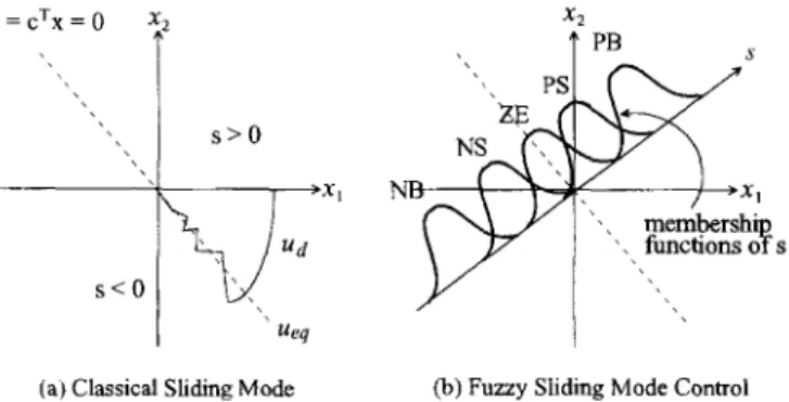
Fig. 1 shows a 2-dimensional case of state plane to illustrate the concept of S M C and FSMC. The sliding surface in Fig. l(a) is a straight line that passes through the equivalent point (0, 0). The state plane has been divided into two parts by the sliding line. One is s > 0, and the other is s < 0. The sliding line is also called the switching line, because the control action switched at the opposite sides of the line. T h a t is why the sliding m o d e control is also known as the variable structure control (VSC). However, such a switching operation has m a n y drawbacks. One of them is the chattering pheno- m e n o n due to the presentations of the system nonideality, such as hysteresis, delay, sampling, un- certainty, etc. To reduce the system nonideality effects, the fuzzification operation was applied to convert the crisp sliding surface into a fuzzy one
s=cTx=0
l 2
s > O:iX 1
S < 0 ~ ' ' , udUeq
X2
,, T PB s(a) Classical Sliding Mode (b) Fuzzy Sliding Mode Control
144 S.-C Lin, Y.-Y. Chen / Fuzzy Sets and Systems 86 (1997) 139-153
[9, 10]. The crisp value of s can be viewed as a gen- eralized distance from a representative point to the sliding surface. Once the s value is fuzzified, a set of fuzzy rules based on the fuzzified distance can be constructed. This is the main idea of the FSMC. Fig. l(b) illustrates such a concept, in which five linguistic labels (PB, PS, ZE, NS, and NB) are assigned to the sliding variable s.
The input and output linguistic labels of the fuzzy sliding mode control rule-base (17) can be determined by certain strategies such as heuristic 1-3,10,13], adaptive [9] or self-organizing [11] methods. However, what is the optimal selection of the membership functions of Sj and Uj? It remains an open problem. In the next section, the para- meters of these fuzzy sets are tuned by means of GAs to derive a sub-optimal F S M C in the sense that the fitness functions are maximized. The main purposes of this paper are:
(1) Apply GAs to search the parameter space of linguistic labels, Sj and Uj, in the fuzzy sliding mode control rule-base (17) for suitable fuzzy control law, uf. The purpose of such a fuzzy control law is to draw the state to hit and slide along the sliding surface without consuming too much control energy.
(2) Derive the hitting control law, Uh, to guaran- tee the stability. During the learning process, if the GA-learned fuzzy control law, uf, is not suitable, such that the state travels toward the direction of divergence, i.e. rsl >~ So, then Ur is turned off, and Uh is turned on to pull the state back to the safe region,
Isl < So.
hand, the Type-II GA-based F S M C tunes all mem- bership functions in the fuzzy control rule-base. The hitting control law in both types of F S M C are identical.
T o improve the performance of GA-based FSMC, the genetic algorithm with elitist model [2] was adopted. Its basic principle is to always include the most fitted individual in the population. The operations are: if the best individual generated up to time t is not in the population of the new genera- tion of time t + 1, then select one member from the new population and replace it with the elitist of the old population.
4.1. Hitting control law Uh
The hitting control law can be used to drive the state to hit the sliding surface wherever the initial state is. To derive the hitting control law, let us set
= 1 and consider a L y a p u n o v function
V =-is2. (19)
The sliding condition [15] which guarantees the stability of a sliding mode control system is
= s ~ < - ~ l s l , (20)
where r / > 0. Suppose that we know the upper bound of f ( ' ) and the lower bound of b, i.e. If[ ~< fmax, 0 < b~in ~< b. Substituting (10) into (20), we have
1/<~ [sbl Ib- l ( f - r ~") + OTx)[ + SbUh. (21)
4. GA-based fuzzy sliding mode controller and stability consideration
In this section, the F S M C with the hitting con- trol law and the fuzzy control law are described in detail. The hitting control law is derived for guaranteeing the system stability; the fuzzy control law is learned by the genetic algorithms. Such kinds of F S M C s are denoted as GA-based FSMCs. Two types of GA-based FSMCs are proposed. In the Type-I GA-based FSMC, only the mem- bership functions in the T H E N - p a r t of the fuzzy control rule-base (17) are adjusted; on the other
To satisfy (20) and (21), the hitting control law can be selected as
Uh = --sign(s)[bmi~(fm.x +
I?")1 + IUxl
+ t/)]. (22) By substituting (22) into (21), the stability condition of (20) can be verified.Remark. Estimating the suitable values of f~ax and
bmi n is an important job for deriving Uh. However,
the precision of the estimation values of these two bounds is dependent on how well the designer understands the system. For example, to control
S.-C Lin, E - E Chen / Fuzo, Sets and Systems 86 (1997) 139 153 145
the f a m o u s inverted p e n d u l u m system,
''~1 = X 2 ,
g sin X l -- (ml/(mc + m ) ) x 22 cos x 1 sin X l
2~'2 = 4
l - (ml/(m~ + m)) cos 2 Xl (1/(me + m ) ) c o s x 1 + ~1 - (ml/(m¢ + m ) ) c o s 2 x l u,
where x~ d e n o t e s the angle of the p e n d u l u m with respect to the vertical line, a n d x2 d e n o t e s the a n g u l a r velocity of the p e n d u l u m . In a real system, the limit values of Xl a n d x2 are always specified. F o r example, Ix1] < 1 t a d a n d ix2] < 4 r a d / s . If we k n o w the structure of the system a n d the variant range of p a r a m e t e r s (e.g. the gravity constant: 9 = 9 . 8 m / s 2 ; the m a s s of the cart: 0 . 8 k g < mc < 1.2kg; the m a s s of the p e n d u l u m : 0.08kg
< m < 0.12kg, the length of the pendulum: 0 . 9 m < l < 1.1 m), then we can calculate the b o u n d s of f a n d b as follows:
[f(x
1, X~)I = g sin x 1 - - (ml/(mc + m))x 2 cos x 1 sin x 1- ~ 1 -- (ml/(mc + m))cos 2 x1 9.8 + ((0.12 × 1.1)/(0.8 + 0.08)) × 42 ~< 10.31 &fm~x, --~l (1/(me + m ) ) c o s x l ] b ( X l ' X 2 ) [ = - - ( m l / ( m c + m ) ) c o s 2 x 1 (1/(1.2 + 0.12))cos 1 ~> 4 x 1.1 - ((0.08 x0.9)/(1.2 + 0.12))cos 2 1 >~ 0.278 & bmi n. U n f o r t u n a t e l y , if we do not have e n o u g h k n o w - ledge a b o u t a system, we c a n n o t estimate the b o u n d s precisely. H o w e v e r , even u n d e r the situ- ation of lacking system i n f o r m a t i o n , we can always a s s u m e t h a t fm~x is very large a n d bmi n is very small. Then, the hitting c o n t r o l Uh can be calculated with- out a n y difficulty. In such a situation, the p o o r e r e s i m a t i o n s of Jm~x a n d b m i n w e t a k e up, the larger Uh
we will get. If the e s t i m a t i o n is t o o p o o r so t h a t the a m p l i t u d e of the hitting c o n t r o l is too large, then Uh will be saturated. T h a t is, Uh b e c o m e s a high gain
b a n g - b a n g control: uh = - s i g n ( s ) [ 7 , where G de- notes the m a x i m a l control input.
F r o m the c o n t r o l law (16), we see that the hitting c o n t r o l Uh plays the role of a protector. T h a t is, w h e n the state lies in the b o u n d a r y layer,
I sl
< So, the G A - l e a r n e d fuzzy c o n t r o l uf is active and the hitting c o n t r o l Uh is disabled; on the o t h e r hand, if uf u n f o r t u n a t e l y does not b e h a v e well such that the state tends to go outside the b o u n d a r y layer, as s o o n as the state hits the b o u n d a r y of the layer, the hitting c o n t r o l b e c o m e s e n a b l e d for driving the state b a c k t o w a r d the layer,4.2. Fuzzy control law uf
T h e fuzzy c o n t r o l law of (16) is given by the following fuzzy sliding m o d e c o n t r o l rule-base:
Rj: I F s is Sj(m],tTi ) T H E N uf is Uj(qo5),
j = 1, 2 . . . N. (23)
R e m a r k . Since the defuzzification m e t h o d a d o p t e d in this p a p e r is the weighted-average, the values of 6j (the second p a r a m e t e r s of Uj) are never used, the search for suitable 6j is not necessary. Hence, for n o t a t i o n a l simplicity, we o m i t 6j here a n d hereafter. H o w e v e r , the values of 6a are required in the center- of-area defuzzification. T h e o p t i m i z a t i o n of '~a a n d their effects are reserved for future research.
F r o m (5) and (6), the fuzzy c o n t r o l law uf of(23) is given by Hf = ~0Vp(s) (24) with ~p = [~01 o2 ... ~0u] x, p(s) = [pl(S) p2(S) ... pu(s)] T a n d psi(s) (25) pj(s) - 2 ~ y , ~,~j(s)
T h e details of learning p r o c e d u r e s of the fuzzy control law in b o t h types of G A - b a s e d F S M C are described as follows:
4.2.1. T y p e - I G A - b a s e d F S M C
T h e fuzzy c o n t r o l law of T y p e - I G A - b a s e d F S M C is given by (24) with adjustable consequence part, q,, a n d fixed premise part, p(s). T h a t is, mj and o) of the m e m b e r s h i p functions in the I F - p a r t of
146 S.-C Lin, E-Y. Chen / Fuzzy Sets and Systems 86 (1997) 139 153 (23) are p r e - d e t e r m i n e d a n d fixed during the learn-
ing period. O n l y the p a r a m e t e r s in the T H E N - p a r t , qgj, are adjusted by GAs. H e n c e the p a r a m e t e r vector, 0, for the genetic a l g o r i t h m is defined as
0 ~ & ~ O = [(/91 (P2 . . . (~0N'] T. (26) Every string in a p o p u l a t i o n c o r r e s p o n d s to an F S M C c a n d i d a t e which has its p a r a m e t e r s e n c o d e d into b i n a r y form. T h e p o p u l a t i o n size is heuristi- cally selected to be M. T h e learning p r o c e d u r e for T y p e - I G A - b a s e d F S M C is s u m m a r i z e d as follows:
Step 1: Define a sliding surface function s = cTx
by carefully selecting the p a r a m e t e r vector c such that (13) is stable a n d satisfies the desired specifications.
Step 2: Define a suitable p e r f o r m a n c e index (cost
function), J. F o r example, it can be defined as
K
J = ~ (w l/s(k)II + v II u(k)II ), (27)
k = l
where k = int(t/At) denotes the iteration instance;
At is the s a m p l i n g period; i n t ( . ) is the r o u n d - o f f o p e r a t o r ; K = int(tmax/At) is the n u m b e r of iter-
ations in one run; t m a x denotes the r u n n i n g time in one run; w and v are positive weights. T h e n o r m
IIll
can be viewed as a generalized energy m e a s u r e of a signal. T h e n the fitness function can be defined as
F = 1/(J + e,o), (28)
where e0 is a small positive c o n s t a n t used to a v o i d the n u m e r i c a l e r r o r of dividing by zero. If the goal is to drive the state to hit the sliding surface as fast as possible regardless of the a m o u n t of c o n t r o l effort required, then the value of w selected w o u l d be significantly larger t h a n that of v. O n the o t h e r hand, the c o n s u m p t i o n of c o n t r o l energy will be p u n i s h e d by h e a v y weighting in u (select a larger v value).
Step 3: Determine: (a) the n u m b e r of rules N; (b)
the p o p u l a t i o n size M; (c) the c r o s s o v e r a n d m u t a - tion rates a n d (d) the bit length d.
Step 4: D e t e r m i n e the p a r a m e t e r values of the
I F - p a r t (mj a n d aj) to f o r m a n u m b e r of G a u s s i a n -
type m e m b e r s h i p functions for s. Heuristics a n d practical c o n s i d e r a t i o n s will be helpful for deciding the values. In Section A.1, we p r o p o s e an a l g o r i t h m
t h a t can be used to d e t e r m i n e mj and aj m a t h -
ematically.
Step 5: D e t e r m i n e the search space of the para-
m e t e r s of the T H E N - p a r t . If the specified range of c o n t r o l signal is [ - [7, +/.7], then t a k e this interval as the search space of (pj.
Step 6: R a n d o m l y generate M p a r a m e t e r vectors
q ¢ ' ) = [~o~ i) qo~ ) ... ~o~ )] (29)
for i = l, 2 . . . M. T h e n the fuzzy c o n t r o l rules of the ith T y p e - I G A - b a s e d F S M C (denoted b y F S M C - I ")) with c o m p l e t e premise parts and ran- d o m c o n s e q u e n c e parts can be constructed, e.g. FSMC-I(~):
( R];): I F s is PB(3, 1.2) T H E N /,/f is
U(/)((~9(/)),
R~': I F s is PM(1.5, 1). T H E N Ur is U~)(qo~)),R~): I F s is N B ( - 3 , 1.2) T H E N uf is
u~)(~o~,)),
(30) where U~ ° are u n k n o w n linguistic labels for c o n t r o l o u t p u t uf; ~o~ i) are adjustable p a r a m e t e r s of U(.0 a n d will be e n c o d e d into the b i n a r y strings for J genetic operations. T h e n the o u t p u t of F S M C - I t~) can be o b t a i n e d by (24).
Step 7: T h e p a r a m e t e r vectors to be tuned by
G A for F S M C - I ") (i = 1,2 . . . M ) are assigned to be
o " ' = ') ... o ? ] T
Step 8: Encode 0J ) (i = 1, 2 . . . M, j = 1, 2, . . . , N )
into d-bit b i n a r y strings B~ i), i.e.
= h ~ (/) (32)
R ( ' ) ( b J v j , ,
--.! . . .
where b) . . . b d • {0, 1}. Then, an individual chro- m o s o m e can be c o n s t r u c t e d by cascading N d-bit b i n a r y strings into a single string as
P(~) = B~)I B~II ... I B~ ). (33)
Step 9: A p o p u l a t i o n can be established as
S.-C. Lin, Y.-E Chen / Fuzzy Sets and Systems 86 (1997) 139 153 147
in which an individual P") corresponds to a set of binary-coded p a r a m e t e r s of an F S M C - I ¢~ which is a candidate of the optimal fuzzy sliding m o d e controller.
Step 10: Use (24) to obtain the fuzzy control part
of F S M C - I "~, i = 1 . . . M, and apply the control law (16) to the plant, where the hitting control law uh is given in (22).
Step 11: Evaluate the performance index and the
fitness function of every F S M C by (27) and (28), respectively.
Step 12: Apply genetic operators (reproduction,
crossover, mutation) to the old population P.
Step 13: Generate a set of offsprings to form
a new population P'. Then apply the elitist model, i.e. c o m p a r e the best fitted strings in the old and the new populations; then r a n d o m l y replace a string in P' with the elitist in P if it has a better fitness value than all individuals in P'.
Step 14: Replace the old population P by the
new population P'.
Step 15: Decode every new individual P") back
to the original p a r a m e t e r space and obtain a set of new p a r a m e t e r 0 (z), i = 1, 2 . . . . , M. Totally, M new Type-I F S M C s are generated by GAs.
Step 16: T a k e ~p"~= 0 ") and repeat Step 10 to
Step 16 until the performance of the best individual satisfies the desired specifications.
4.2.2. T y p e - I I GA-based F S M C
The fuzzy control law of T y p e - I I G A - b a s e d F S M C is given by (24) with both adjustable conse- quence part, q~, and premise part, p(s). Both mj, aj in the I F - p a r t and q)j in the T H E N - p a r t of (23) are adjusted during the learning period. Hence, the p a r a m e t e r vector, 0, of the genetic algorithm can be written as
0 = [ ' m T ~ ' T ~ 0 T ] T
= [ m 1 m 2 ... rnN o-1 0"2 ... O-N q~l q~2 --- ~PN] T"
(35)
Basically, the learning procedure of T y p e - I I G A - based F S M C is similar to that of Type-I. It is described as follows:Step 1-Step 3: Same as Step 1-Step 3 in the
learning procedure of Type-I G A - b a s e d FSMC.
Step 4: Determine the search space of m: and o-j.
See Section A.2.
Step 5: Same as Step 5 in the learning procedure
of Type-I G A - b a s e d FSMC.
Step 6: R a n d o m l y generate 3M p a r a m e t e r
vectors:
I
r a ( i ) = Em(il , m ~ ) ... m ~ ) ] TO " ( i ) = Eo'i/) O-(~) . 0"~)3 T ( 3 6 )
~[~(i)= [~9(i/) ~0~ ) ... (~O~)] T
for i = 1,2, . . . , M. Then the fuzzy control rules of the ith T y p e - I I G A - b a s e d F S M C (denoted by F S M C - I I "~) with r a n d o m premise and conse- quence parts can be constructed as
F S M C - I I %
R]i': IF s is S~)(m~li),o-~ )) THEN /,/f is U(li)(q~([)),
02 v"2 ,~2.J THEN uf is ~z ~ 2 J'(37) R~): IF s is S!~'(m~),a~ )) THEN uf is U~)(tp~)),
where _j S¢. ° and I:~! _ : ) are u n k n o w n linguistic labels for input variables s and control output uf, respec- tively; mj~/), a j") and ~0j") are adjustable parameters of 5;(: ) and - - j U(. ° - - j , and will be encoded into the binary strings for genetic operations. Then the fuzzy con- trol part of F S M C - I I Cz) can be obtained by (24).
Step 7: The p a r a m e t e r vectors to be tuned by
G A for F S M C - I I ") (i = 1,2, . . . , M) are assigned as
.,. " ~ ( i ) -~o(i)
0~)]T
o(o= Eo >
. .. . . . .: = E r a ? . . . . . . ' ) . . .
= Em(i)Ti~(i)T i ~O(1)T] T. (38)
Step8: Encode 0ql (i = 1,2, v j . . . , M , j = 1,2 . . . . ,3N)
into d-bit binary strings Re: ) _ j as shown in (32), and then cascade 3N d-bit binary strings into an indi- vidual string
. . . . " . . .
~(i)
• ~ ( i )
B ~ + l i "'" i - 3 N .
Step 9: A population can be established as
p = {p(1), p(2) . . . p(M)},
(39)
148 S.-C. Lin, E-Y. C h e n / Fuzzy Sets and Systems 86 (1997) 139-153
in which an individual P") c o r r e s p o n d s to a set of b i n a r y - c o d e d p a r a m e t e r s of an F S M C - I I ") which is a c a n d i d a t e of the o p t i m a l fuzzy sliding m o d e controller.
Step 10: Use (24) to o b t a i n the fuzzy c o n t r o l law o f F S M C - I I (i), i = 1 . . . M. T h e n apply the c o n t r o l law (16) to the plant, where the hitting c o n t r o l law uh is given by (22).
Step 11 S t e p 15: Same as Step 11 Step 15 in the learning p r o c e d u r e of T y p e - I G a - b a s e d F S M C .
Step 16: Take m ( i ) = [0(/) . . . 0 ~ ) ] T, tlr t i ) =
r 0 ~ ) + 1 . . . ~ 2 N I ~(i) aT and tp <i) = L ~ 2 N + I
r~q(i)
. . .0~)N] T,
andrepeat Step 10 to Step 16 until the p e r f o r m a n c e of the best individual satisfies the desired specifications.
C o m p a r i n g with T y p e - I a n d T y p e - I I approaches, T y p e - I I is m o r e flexible t h a n Type-I, but T y p e - I is m o r e efficient than Type-II. First, the search space is merely c o n s t r u c t e d by the p a r a m e t e r strings of the T H E N - p a r t in the T y p e - I a p p r o a c h , while it is c o n s t r u c t e d by the I F - p a r t a n d the T H E N - p a r t p a r a m e t e r strings in the T y p e - I I a p p r o a c h . O b - viously, the f o r m e r is m u c h smaller t h a n the latter. Secondly, the e n c o d e d length of bit strings in the T y p e - I a p p r o a c h is m u c h shorter t h a n that in T y p e - II, such that the c o m p u t a t i o n load of the T y p e - I a p p r o a c h is less h e a v y t h a n that of Type-II. There- fore, if w h a t we w a n t is just an acceptable result instead of a best one, the T y p e - I a p p r o a c h will be a better choice.
5. Simulation results and discussions
In this section, we examine the p e r f o r m a n c e of o u r m e t h o d s by a n u m b e r of examples. C o n s i d e r a s e c o n d - o r d e r n o n l i n e a r system with the d y n a m - ical e q u a t i o n in the following:
my: + f l ( y 2 _ 1)3;' + k y = u, (41)
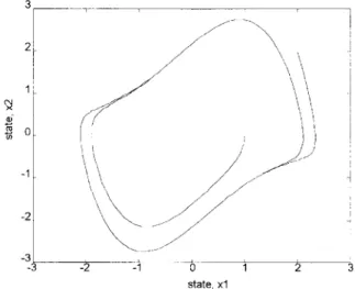
where u a n d y d e n o t e the system input a n d o u t p u t , respectively, m, c a n d k are positive constants. Eq. (41) can be regarded as the description of a mass spring d a m p e r system with a position- d e p e n d e n t d a m p i n g coefficient fl(y2 _ 1), or, equiv- alently, an R L C electrical circuit with a n o n l i n e a r resistor. W i t h m = 1 and k = 1, the unforced system (u = 0) b e c o m e s the f a m o u s Ven der P o l oscillator
3 2 I ~ - ' ~ ' ¸ ' ' ~ I 1L -,~ 0 -1 -3 -3 3
\ ,
\, q "~l! k / -2 -1 % i state, xlFig. 2. The unforced system behaves as a Ven der Pol oscillator.
[15]. If the states are defined to be Xl = y, a n d x2 = d y / d t , then the state trajectory of the unforced system with fl = 1 has a limit cycle, as shown in Fig. 2. Assume that the specified input voltage (force) is between [ - 30, 30]. In o u r d e m o n s t r a t i o n , the c o n t r o l goal is to drive the state t o w a r d the sliding surface, a n d slide along it so that xl and x2 a p p r o a c h zero as t a p p r o a c h e s infinity.
In the following simulations, the sliding surface function is selected as s = xl + x2, the b o u n d a r y layer is selected as [ - - 3 , 3], a n d the initial condi- tions are xl(0) = 3 a n d x2(0) = 0. The p r o t o t y p e of fuzzy c o n t r o l rule-base has six rules (N = 6), de- fined as follows:
R / I F s is Sj(mj, a~) T H E N b/f is Uj(~oj),
j = 1, 2 . . . 6. (42)
T h e p o p u l a t i o n size M = 10; the crossover a n d m u t a t i o n rate are selected as 0.8 a n d 0.01, respec- tively.
A c c o r d i n g to (27), select w = T A k . At, v = 2, a n d use the /l-norm. If t .... = 6 s a n d At = 5 ms, then K = 1200 a n d the cost function becomes
1 2 0 0
J = ~" ( T l s ( k ) [ + 2lu(k)l). (43)
k--1
C o m p a r i n g with the equal-weighted case (w = v = 1), in (43) while T is small, the weight of the c o n t r o l
S.-C. Lin, E - E Chen / Fuzzy Sets and Systems 86 (1997) 139-153 1 4 9
signal is larger than that of the sliding function, so that the controller which can reserve more control energy gets higher fitness. However, as time pro- gresses, T is larger and larger. Hitting and sliding become more and more important than energy conservation. Consequently, the controller which can pull the state closer to the sliding surface gets a higher score. In conclusion, the controller which can drive the state toward the surface quickly and does not dissipate too much control energy will yield higher fitness.
The following two examples are presented to illustrate the learning results of Type-I and Type-II GA-based FSMC, respectively.
Example 1 (Type-I
GA-based FSMC).
By the EPA (Equal Partition Algorithm, see Section A.1), it is easy to determine the value of the IF-part parameters. Assume that the membership grade of crossover point is /t = 0.6, then we have{Sj(mj, aj)lj
= 1,2, . . . , 6 } = { N B ( - 3 , 0 . 8 4 ) ,N S ( - 1.8, 0.84), N Z ( - 0 . 6 , 0 . 8 4 ) , PZ(0.6, 0.84), PS(1.8, 0.84), PB(3, 0.84)}.
Since the range of system input is [ - 30, 30], that implies the amplitude of controller cannot exceed the interval. It is reasonable to select the universe of the discourse of q0j to be within the interval [ - 30, 30]. In the Type-I approach, the parameters to be learned by GAs are 0 i := q~j (j = 1,2 . . . 6). The initial population is generated by a random number generator. If every parameter is encoded to an 8-bit (d = 8) binary string, then cascading six strings of (01, 02 . . . 06) forms a 48-bit chromo- some.
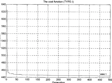
Fig. 3 shows the evaluation process of the cost function of the best individual. We can see that the cost function indeed decreased from generation to generation. The decoded values of the best indi- vidual in the generation 500 are shown in Table 1. It is the final parameter set of Type-I GA-based F S M C that we want. If each output linguistic label Uj is assigned an appropriate physical meaning such as NB and PS based on the values of ~0j, then the final fuzzy rule-base and membership functions
6 4 0 6 2 0 6 0 0 5 8 0 T h e c o s t f u n c t i o n ( T Y P E - I ) 5 6 0 . _ o "5 5 4 0 o 5 2 0 I I t I I . . . . "T . . . . I I . . . . J~ . . . . t t . . . . ,+ . . . . I I I . . . . "r - - - I I I I I I I I I L I I I I I . . . I ... " t . . . t . . . I ... ~ . . . t t t I I I r i I I I { . . . i ... t . . . i ... _ [ . . . i f t t i f t i i i i i . . . i . . . i . . . i . ... . e . . . 0 ~ t i i i f i I I t I . . . I . . . I . . . I . ... 1 . . . t I I I I I I q I I i I I I - I . . . . 7 . . . ~ . .. . . .. . . ~ . . . ~ . . . '7 . . . J t r I J I t I I I 5 0 0 - - - • . . . ~ . . . -L . . . ~ . . . r . . . 4 . . . . I ~ I b q I ' 1 ' ' I ' I I I I 4 8 0 . . . . - t ......... t ......... ~ . . . ~ . . . E . ........ " r . . . . I ~ I t I I I I I t t t I t t 4 6 0 . . . . 7 . . . . " . . . ~ . . . 7 . . . ~ . . . 5 . . . . . ~ . , ~ . . ~ 4 4 4 . 1 4 4 0 i ~ i i I I 5 0 1 0 0 1 5 0 2 0 0 2 5 0 3 0 0 3 5 0 4 0 0 4 5 0 5 0 0 Generation F i g . 3 . T h e c o s t f u n c t i o n ( T y p e - I ) .
150 S.-C. Lin. }1-}1 C h e n / Fuzzy Sets and Systems 86 (1997) 139 153
Table 1
The final parameter sets of the Type-I GA-based FSMC
~l ~2 ~a ~4 ~5 ~6
--2.9412 --30 --21.5294 21.7647 29.2941 27.1765
for the F S M C may look like:
RI: 1F s is NB(-3,0.84) THEN uf is NS(-2.9412), R2: IF s is NS(-1.8,0.84) THEN uf is NB(-30), R3: I F s is N Z ( - 0 . 6 , 0 . 8 4 ) T H E N uf is N M ( - 2 1 . 5 2 9 4 ) , R4: I F s is PZ(0.6,0.84) T H E N uf is PZ(21.7647), Rs: I F s is PS(1.8,0.84) T H E N ur is PB(29.2941), g 6 : I F s is PB(3,0.84) T H E N uf is PM(27.1765).
Finally, the state trajectory and the control signal of the fuzzy sliding mode control system are shown in Fig. 4.
Example 2 (Type-II GA-based FSMC). According to the strategy in Section A.2, the search space of
o -0.5 -1 -1.5 -2 -2.5 o
(a) State response (TYPE-I)
I I I - - - I . . . T . . . i . . . . T . . . " l I I I I i I . . . ~ ... .... .... d r I I 1 2 3 4 state, xl 10 0 . - 1 0 8 -20 -30
(b) Control signal (TYPE-I)
I I I
2 4 6
time (sec)
Fig. 4. The state response and the control signal of the Type-I GA-based FSMC.
The cost function (TYPE-II) 650 600 = 5501 .o "5 fi o 500 450 400 . . . ~ . . . . I I I I I . . . L . . . . " - 1 . . . . I I I I - A . . . I I t I r / - - - 7 .. .. ... . @ . . . . . I I I I I I I I I I I I I 50 100 150 200 250 - - - 1- . . . . I I I I . . . . / . . . . | 300 I I I I I I t . . . I i ~ 3 - - 8 ~ 8 - - - I I I I I I I I I I 350 400 450 Generation
Fig. 5. The cost function (Type-ll).
S.-C. Lin, Y.-Y. Chen / F u z z y Sets a n d S y s t e m s 86 (1997) 139 153 151
mj, aj and q)j are selected as [ - 3 , 3 ] , [0.5, 1.5] and [ - 30, 30], respectively. The parameters of premise and consequence parts, mi, ai, ~0j, were encoded to 8-bit binary strings, respectively. Therefore, cascad- ing 18 strings of(m1, . . . , m6, or1, . . . , ~r6, q)l . . . . , q)6) forms a 144-bit individual. Because the number of adjustable parameters in Type-II is larger than that in Type-I, we may expect that the final controller learned by Type-I! would be better than that by Type-I.
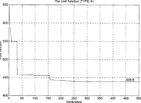
Fig. 5 shows the evaluation process of the cost function of the best individual. Again, the cost function decreased from generation to generation. Comparing Fig. 5 with Fig. 3 we see that the min- imum of the cost function in Type-II (438.8) is smaller than that in Type-I (444.1), but the conver- gence rate of Type-II is slower than that of Type-I. The decoded values of the best individual in the generation 500 are shown in Table 2. It is the final parameter set of Type-II GA-based F S M C that we want. If each linguistic label is assigned with an appropriate physical meaning such as NB and PS
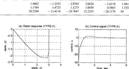
based on its value, then the final fuzzy rule-base and membership functions for the F S M C may look like: RI: 1F s is PM(1.9882, 1.1784) THEN uf is PM(29.5294), R2: IF s is N S ( - 1.2353, 1.4725) THEN ur is N S ( - 11.4118), R3: IF s is NB(-2.9765,1.1275) THEN uf is NB(-29.7647), R,,: IF s is PB(2.0824, 1.0059) THEN uf is PS(22,2353), R s: IF s is N M ( - 1.6118,0.5863) THEN uf is NM(-28.1176), R6: IF s is PS(1.9412,1.3353) THEN uf is PB(30.0000). Finally, the state trajectory and the control signal of the fuzzy sliding mode control system are shown in Fig. 6.
We had also simulated the design examples un- der the conditions of different GA parameters. In general, mutation rate e [0.005, 0.01] and cross- over r a t e ~ [0.75,0.95] (see [14]). However, we cannot include the complete results due to limited space. The GA parameters selected in this paper are typical values as seen in many related researches. In our simulations, we found that a higher mutation
Table 2
The final parameter sets of the Type-II GA-based FSMC v a l u e ~ i n d e x j 1 paramete-r- - ~ 2 3 4 5 6 m~ 1.9882 --1.2353 1.1784 1.4725 ~ 29.5294 --11.4118 --2.9765 2.0824 --1.6118 1.9412 1.1275 1.0059 0.5863 1.3353 --29.7647 22.2353 --28.1176 30 0 -0.5 -1 -1.5 -2 -2.5
(a) State response (TYPE-II)
- - - - t ... T . ... ... I I I I ... I ... ~ z - - - I ... I I I I I I 1 2 3 4 state, xl 10
(b) Control signal (TYPEql)
O -10 . . . "E 8 - 2 0 . . .. . . . .. . . . .. . . . .. . . . -3C 0 2 6 time, sec
1 5 2 S.-C. Lin, E - E Chen / Fuzo, Sets andSvstems 86 (1997) 139 153
rate m a y yield a higher probability to escape the local m i n i m u m but m a y break the better schemata. The larger population size contains sufficient in- formation for finding the solution but takes a very long time to evaluation and causes heavy c o m p u t a - tion load. M o r e details of the effects of G A para- meters can be found in [1, 14].
6. Conclusions
experimentally in hard disk servo control as well as XY table precision positioning in the near future.
Appendix A
This appendix gives one of the possible methods to determine the universe of discourse as well as the values of the parameters mi and o~i in the IF-part. In this paper, we have shown a genetic algorithm
with the elitist model that indeed behaves as an efficient searching tool for finding a sub-optimal fuzzy sliding m o d e controller. Two types of GA-based learning algorithms for F S M C s are discussed. In the T y p e d approach, only the parameters in the T H E N - p a r t are learned, while all the parameters in both the I F - p a r t and the T H E N - part are considered in the T y p e - I I approach. The Type-I a p p r o a c h has the advantages of a shorter string length and a smaller search space such that its convergence rate is faster than Type-II. The shortcoming is that the I F - p a r t of the rule-base has to be pre-defined heuristically. However, an Equal Partition Algorithm is proposed to determine the I F - p a r t mathematically. On the other hand, the T y p e - l l a p p r o a c h has a longer string length by including more parameters to be learned in the rule-base. The I F - p a r t need not be defined a priori and can be tuned by the genetic algorithm. It leads the T y p e - I I a p p r o a c h to have a greater possibility of finding the global m i n i m u m than Type-I, but the convergence rate m a y be slower.
The most important advantage of introducing the sliding m o d e into fuzzy control is that the dynamic behavior of a fuzzy control system can be specified and dominated by the user-defined sliding surface. Moreover, an M I S O fuzzy controller can be transformed into an SISO fuzzy sliding m o d e controller by combining the system states into a single sliding variable. The n u m b e r of control rules can be reduced to a linear function of the n u m b e r of input variables. Hence, the string length used to learn an F S M C is shorter than that used to learn a conventional FLC.
The proposed algorithms are currently under hardware i m N e m e n t a t i o n and will also be tested
A.I. Equal Partition Algorithm for Type-I
GA-based F S M C
In the T y p e d G A - b a s e d FSMC, one of the most i m p o r t a n t jobs is to decide how to partition the I F - p a r t and then determine the values ofmj and aj. First, we have to determine the range ofmi. F r o m (9), we have
Is[ ~< ~ Icil Ixil ~< ~
]ci[-~i~So,
i 1 i 1
where the ci's are design parameters, given by the designer; 2"i denotes the upper (safe) bound of [xgJ and can be obtained from the system specification. Therefore, the b o u n d a r y layer I - s o , s o l is easy to calculate and the universe of discuss ofmj can be set to be [ - S o , S 0 ] directly. Next, for simplicity, the values of m/s are obtained by equally dividing the interval into N - 1 partitions, that is
m i = ( - s o ) + (j - 1)A,
where N is the n u m b e r of membership functions and A = 2 S o / ( N - 1) is the width of the partition.
Secondly, to determine the value of a~, let us consider the simplest case that every Gaussian-type membership function in the I F - p a r t has equal vari- ant, i.e. a j ~ a , Vj. By definition, we can get the value of a by solving any two equations of adjacent membership functions:
and
s . - c Lin, K-K Chen / Fuzzy Sets and Systems 86 (1997) 139 153 153 A s s u m e t h a t t h e m e m b e r s h i p g r a d e o f t h e c r o s s o v e r p o i n t o f t h e s e t w o a d j a c e n t m e m b e r s h i p f u n c t i o n s is p, t h e n w e h a v e a = - [ ~ ) / ( l n # ) . A.2. D e t e r m i n e the s e a r c h s p a c e o f m r a n d c 0 in T y p e - l l G A - b a s e d F S M C In t h e T y p e - I I G A - b a s e d F S M C , w e h a v e t o d e t e r m i n e t h e s e a r c h s p a c e o f mj a n d aj s u c h t h a t G A s c a n s e a r c h on, It is r e a s o n a b l e t o c h o o s e t h e s e a r c h s p a c e as m ~ [ - S o , S o l a n d aj ~ [q, 6], w h e r e A 2/' _ in w h i c h / 3 a n d fi a r e t h e l o w e r a n d u p p e r m e m b e r - s h i p g r a d e s o f t h e c r o s s o v e r p o i n t s . F o r e x a m p l e , _ p = 0 . 1 a n d f i = 0 . 9 . R e f e r e n c e s
I l l T. Back, Optimal mutation rates in genetic search, Proc. 5th lnternat. Cot!f on Genetic Ah.lorithms (1993) 2 8. [2] D.E. Goldberg, Genetic Algorithms in Search, Optimization,
and Machine Learning (Addison-Wesley, Reading, MA, 1989).
[3] G.C. Hwang and S.C. Lin, A stability approach to fuzzy control design for nonlinear systems, Fuzzy Sets and Systems 48 (1992) 279 287.
[4] U. ltkis, Control System qf Variable Structure (Wiley, New York, 1976).
[5] C.L. Karr, Genetic algorithms for fuzzy controller, Al Expert 6 (Feb. 1991) 26-33.
[6] C.L. Karr, Applying genetics to fuzzy logic, AI Expert 6 (Mar, 1991) 38-43.
[7] K. Kristinsson and G.A. Dumont, System identification and control using genetic algorithms, IEEE Trans. Sys- tems Man Cybernet. SMC-22 (1992) 1033- 1046. [8] C.C. Lee, Fuzzy logic in control systems: fuzzy logic con-
troller, Parts I and II, IEEE Trans. Systems Man Cybernet. SMC-20 (1990) 404--435.
[9] S.C. Lin and Y.Y. Chen, Design of adaptive fuzzy sliding mode for nonlinear system control, Proc. IEEE lnternat. Cor{f on Fuzzy Systems, Orlando (1994) 35 39.
[10] S.C. Lin and C.C. Kung, A linguistic fuzzy-sliding mode controller, Proc. ACC 3 (1992) 1904 1905.
[11] Y.S. Lu and J,S. Chen, A self-organizing fuzzy sliding- mode controller design for a class of nonlinear servo systems, IEEE Trans. Industrial Electronics 41 (1994) 492 502.
[12] E.M. Mamdani, Application of fuzzy algorithms for con- trol of simple dynamic plant, Proc. lEE 121 (1974) 1585 1588.
[13] R. Palm, Sliding mode fuzzy control, Proc. IEEE lnternat. Conf on Fuzzy Systems, San Diego (1992) 709 715. [14] J.O. Schaffer, R.A. Caruana, LJ. Eshelman and R. Das,
A study of control parameters affecting online perfor- mance of genetic algorithms for function optimization, in: J.D. Schaffer, Ed. (1989) 51 60.
[15] J.J.E. Slotine and W. Li, Applied Nonlinear Control (Prentice-Hall, Englewood Cliffs, NJ, 1991).
[16] M. Sugeno and M. Nishida, Fuzzy control of model car, Fuzzy Sets and Systems 16 (1985) 103 113.
[17] R. Tanscheit and E.M. Scharf, Experiments with the use of a rule-based self-organizing controller for robotic applica- tions, Fuzzy Sets and Systems 26 (1988) 195 214. [18] D.M. Tate and A.E. Smith, Expected allele coverage and
the role of mutation in genetic algorithms, lnternat. Conf. on Genetic' Algorithms (1993) 31 37.
[19] V.I. Utkin, Slidin9 Modes and Their Application in Vari- able Structure System (Mir Press, Moscow, English trans- lation, 1978).
[20J L.A. Zadeh, Outline of a new approach to the analysis of complex systems and decision processes, IEEE Trans. Systems Man Cybernet. SMC-3 (1973) 28 44.