適應性背景重建技術用於多目標追蹤系統與其在交通參數擷取之應用

全文

(1)國立交通大學電機資訊學院電機與控制學程碩士論文. 適應性背景重建技術用於多目標追蹤系統與其在交通參數擷取之應用 Multi-objects Tracking System Using Adaptive Background Reconstruction Technique and Its Application to Traffic Parameters Extraction. 研究生：黃裕程指導教授：林進燈教授. 中華民國九十四年七月.

(2) 適應性背景重建技術用於多目標追蹤系統與其在交通參數擷取之應用 Multi-objects Tracking System Using Adaptive Background Reconstruction Technique and Its Application to Traffic Parameters Extraction. 研究生：黃裕程. Student：Yu-Chen Huang. 指導教授：林進燈教授. Advisor：Prof. Chin-Teng Lin. 國立交通大學. 電機資訊學院電機與控制學程碩士論文 A Thesis Submitted to Degree Program of Electrical Engineering and Computer Science College of Electrical Engineering and Computer Science National Chiao Tung University in Partial Fulfillment of the Requirements for the Degree of Master of Science in Electrical and Control Engineering July 2005 Hsinchu, Taiwan, Republic of China. 中華民國九十四年七月.

(3) 適應性背景重建技術用於多目標追蹤系統與其在交通參數擷取之應用. 學生：黃裕程. 指導教授：林進燈教授. 國立交通大學電機資訊學院電機與控制學程﹙研究所﹚碩士班. 摘. 要. 在最近幾年，隨著車輛與其他交通工具的快速發展與普及化，各地的交通狀況也日趨繁忙與混亂。因此，為了改善或有效控管交通狀況，智慧型運輸系統（Intelligent Transportation Systems ,ITS）變成一個在學術研究和業界開發中十分重要的領域。而在傳統的交通監測系統，其監測方法在資料的擷取或系統擴展空間上均表現不佳。而監測系統如同整個系統的眼睛，必須扮演自動檢測出車輛及行人同時持續地追蹤他們的角色。藉由追蹤系統獲得的資訊，ITS 可以執行進一步的分析來使得系統有效率地進行有效決策以改善交通狀況。在這篇論文中，我們提出了一個多目標的即時追蹤系統，它可以在固定式攝影機獲得的交通監視影像中，進行移動物體的檢測。配合適應性背景重建技術，系統可以有效地處理外界光線或其他環境的變化來達到良好的物體擷取結果。另外，我們將擷取出來的物體特徵搭配以區塊為基礎的追蹤演算法來達到物體持續追蹤的目的，也可以正確地追蹤發生重合或分離情形的物體。得到追蹤的結果後，我們可以進一步分析物體的特性及行動來產出有用的交通參數。針對我們提出的系統架構，我們實作了一個監測系統並包括移動物體分類及事故預測的功能。我們以實際的路口交通影像與其他監測影像樣本來進行實驗，實驗結果證明我們所提出的演算法與系統架構達成了強健性的物體擷取結果並在重合及分離的情況下成功地追蹤物體。同時也正確地擷取了有用的交通參數。. i.

(4) Multi-objects Tracking System Using Adaptive Background Reconstruction Technique and Its Application to Traffic Parameters Extraction. Student：Yu-Chen Huang. Advisors：Prof. Chin-Teng Lin. Degree Program of Electrical Engineering Computer Science National Chiao Tung University. ABSTRACT. In recent years, the traffic situation is busy and chaotic increasingly everywhere because of high growth and popularization of vehicles. Therefore, intelligent transportation systems (ITS) become an important scope of research and industrial development in order to improve and control the traffic condition. In traditional traffic surveillance systems, their monitoring methods are inefficient in information extraction and short of improving. A tracking system is like ITS’ eyes and it plays the role of detecting vehicles or pedestrians automatically in the traffic scene and tracking them continuously. According to results of tracking systems, ITS can do further analysis and then perform efficient and effective actions to make the traffic condition better. In this thesis, we present a real-time multi-objects tracking system and it detects various types of moving objects in image sequences of traffic video obtained from stationary video cameras. Using the adaptive background reconstruction technique we proposed can effectively handle with environmental changes and obtain good results of objects extraction. Besides, we introduce a robust region- and feature-based tracking algorithm with plentiful features to track correct objects continuously and it can deal with multi-objects occlusion or split events well. After tracking objects successfully, we can analyze the tracked objects’ properties and recognize their behavior for extracting some useful traffic parameters. According to the structure of our proposed algorithms, we. ii.

(5) implemented a tracking system including the functions of objects classification and accident prediction. Experiments were conducted on real-life traffic video of some intersection and testing datasets of other surveillance research. The results proved the algorithms we proposed achieved robust segmentation of moving objects and successful tracking with objects occlusion or splitting events. The implemented system also extracted useful traffic parameters.. iii.

(6) 誌謝首先，最感謝的是我的指導教授林進燈博士，在我的研究學習過程中，能夠不辭辛勞地給予我適時的指導與幫助。而在我必須同時兼顧工作與研究的狀況下，林教授的支持與鼓勵讓我可以有動力持續地進行研究工作，再次感謝他的教誨與支持。另外，蒲鶴章博士以及諸位學長們的悉心鞭策，也使我在各方面均有長足的進步，在此感謝他們無私的指導與協助。而莊仁輝教授、林正堅教授等口試委員給予了許多寶貴的意見，使本論文可以更加完備，在此深深致謝。在我忙於工作與研究之際，常常佔用了許多與家人分享同歡的時間，而我的家人總是以無盡的體貼與關懷來包容我，尤其和我的妻子楊慧萍小姐間之相互扶持與鼓勵，讓我可以在低潮瓶頸中突圍而出，衷心感謝他們。雖然我的母親在我這段的求學過程中離開了，但是我還是希望與她分享一路走來的苦樂與努力，也感謝她多年以來辛勞地照顧培育我。還有，感謝實驗室的同學弘昕、宗恆、Linda、盈彰、峻永與其他伙伴，大家的互相砥礪與切磋，產生許多研究上的火花與生活的樂趣，希望未來的日子還有相聚合作的機會。而工作上長官與同事的配合與體諒，使我減少了工作與學業間的衝突，在此一併謝謝他們的慷慨仁慈。雖然，只是短短的三年時光，但是要感謝的人還是難以一一說明，最後感謝大家這段時間來的幫忙，讓我深深感受你們的溫暖與熱情。. 黃裕程交通大學 July, 2005. iv.

(7) Table of Contents Abstract in Chinese.....................................................................................................................i Abstract in English .....................................................................................................................ii Acknowledgements in Chinese .................................................................................................iv Table of Contents........................................................................................................................ v List of Figures............................................................................................................................vi List of Tables ............................................................................................................................vii Chapter 1 Introduction................................................................................................................ 1 1.1 Motivation and Contribution .................................................................................. 1 1.2 Organization ........................................................................................................... 2 Chapter 2 Related Work.............................................................................................................. 3 2.1 Objects Extraction .................................................................................................. 3 2.2 Objects Tracking..................................................................................................... 6 2.3 Behavior Analysis .................................................................................................. 8 Chapter 3 Multi-objects Tracking System with Adaptive Background Reconstruction........... 11 3.1 System Overview.................................................................................................. 11 3.2 Foreground Segmentation .................................................................................... 12 3.2.1 Background Initialization ......................................................................... 13 3.2.2 Adaptive Background Updating ............................................................... 15 3.2.3 Background Subtraction ........................................................................... 17 3.3 Objects Extraction ................................................................................................ 18 3.3.1 Pre-Processing .......................................................................................... 19 3.3.2 Connected Components Algorithm .......................................................... 20 3.3.3 Objects List............................................................................................... 21 3.4 Objects Tracking................................................................................................... 22 3.4.1 Matching Analysis .................................................................................... 24 3.4.2 Objects Merging ....................................................................................... 25 3.4.3 Objects Splitting ....................................................................................... 27 3.4.4 Other Matching Processes ........................................................................ 28 3.4.5 Current Objects List Updating.................................................................. 30 3.4.6 Life and Status of Objects ........................................................................ 30 3.5 Behavior Analysis................................................................................................. 32 3.5.1 Camera Calibration and Object Classification ......................................... 32 3.5.2 Accident Prediction .................................................................................. 34 Chapter 4 Experimental Results ............................................................................................... 38 4.1 Results of Background Reconstruction and Foreground Segmentation............... 38 4.1.1 Background Initialization ......................................................................... 38 4.1.2 Adaptive Background Updating ............................................................... 40 4.2 Results of Objects Tracking.................................................................................. 44 4.2.1 Objects Tracking....................................................................................... 44 4.2.2 Occlusion and Splitting of Multiple Objects ............................................ 45 4.2.3 Stopped Objects........................................................................................ 48 4.3 Behavior Analysis................................................................................................. 51 Chapter 5 Conclusions.............................................................................................................. 54 References ................................................................................................................................ 56. v.

(8) List of Figures Fig. 1 Global system diagram …………………………………………………………….. 11 Fig. 2 The process diagram of foreground segmentation …………...…………………….. 14 Fig. 3 The calculating scope for the index of adaptive threshold ………………………..... 16 Fig. 4 Diagram of object extraction process ………………………………………………. 19 Fig. 5 Diagram of establishing objects list ………………………………………………... 19 Fig. 6 Overlap area between current object and previous object …………………………. 22 Fig. 7 Diagram of tracking process ……………………………………………………….. 23 Fig. 8 Diagram of simplifying overlap relation list .………………………………………. 24 Fig. 9 Objects history of objects merging ………………………………………………… 26 Fig. 10 Diagram of objects merging ……………..……………………………………….. 26 Fig. 11 Objects history of object splitting ……..………………………………………….. 27 Fig. 12 Process of object splitting …………………..…………………………………….. 28 Fig. 13 Process of extended scope matching ……………………………………………… 29 Fig. 14 Diagram of isolated objects process ………..…………………………………….. 29 Fig. 15 Diagram of life feature ..………………..…………………………………………. 31 Fig. 16 Diagram of behavior analysis …………….……………………………………….. 32 Fig. 17 Diagram of modified bounding box ……………………………………….……… 33 Fig. 18 Diagram of type I of the relation of two objects ………………………………….. 35 Fig. 19 Diagram of type II of the relation of two objects …………………………………. 36 Fig. 20 Diagram of type III of the relation of two objects ………………………………… 37 Fig. 21 Temporary background images during background initialization ………………… 40 Fig. 22 Experimental results of background updating (#2212~#2234) ………………..….. 42 Fig. 23 Experimental results of background updating (#3300~#3580) …………………… 43 Fig. 24 Experimental results of objects tracking (#500~#700) …………..……………….. 44 Fig. 25 Tracking results of PETS2001 dataset1 (#2760~#2960) ………………… ………. 45 Fig. 26 Experimental results of objects with occlusion and split events ………..………… 46 Fig. 27 Experimental results of occlusion and split of multiple objects ……………..….… 48 Fig. 28 Tracking results of stopped objects …..……………………………………….…... 51 Fig. 29 The outlook of the implemented program ………………………………………… 51 Fig. 30 Experimental results of objects classification ….…………………………………. 52 Fig. 31 Experimental results of accident prediction ……………………………………… 53. vi.

(9) List of Tables Table 1 Phases of adaptive background updating …………………………………………. 16 Table 2 Rule of objects classification ……..………………………………………………. 34. vii.

(10) Chapter 1 Introduction 1.1 Motivation and Contribution In recent years, the traffic situation is busy and chaotic increasingly everywhere because of high growth and popularization of vehicles. How to improve and control the traffic condition with advanced techniques is one of the most important missions among the developed countries. Therefore, intelligent transportation systems (ITS) became an important scope of research and development in academia and industries. Traditional traffic surveillance systems often use sensors to detect passing of vehicles and gather simple information or use fixed cameras to record video and check the video by eyes when some events happened. Those methods are inefficient in information extraction and short of improving. Vehicles and pedestrians are the basic units of ITS’ structure. Thus, a tracking system of vehicles or pedestrians is a key module of ITS. It’s like ITS’ eyes. It plays the role of detecting vehicles or pedestrians automatically and of tracking them continuously in the traffic scene. According to results of tracking systems, ITS can do further analysis and then perform efficient and effective actions to make the traffic condition better. In this thesis, we present a real-time multi-objects tracking system. Firstly, it can detect various types of moving objects in image sequences obtained from stationary video cameras and moving objects are segmented from the images. Using the adaptive background reconstruction technique we proposed can effectively handle with noise effects, illumination, and/or environmental changes and obtain good results of objects extraction. Secondly, we introduce a robust tracking algorithm which combines region-based method and feature-based method to track objects correctly and this algorithm can deal with multi-objects occlusion or. 1.

(11) splitting events well. After tracking objects successfully, we can analyze the tracked objects’ properties and recognize their behaviors for extracting some useful traffic parameters. In our implementation, we use the estimation of trajectories to obtain information for accident prediction. Besides, the tracking system can provide the data ITS required and extend its architecture to combine with other sub-systems of ITS. In brief, a good tracking system means wider surveillance scope and higher accuracy of objects’ information and is indispensable to any implementation of ITS or surveillance systems.. 1.2 Organization This thesis is organized as follows: Chapter II gives an overview of related work about this research realm and presents the research by different modules. Chapter III introduces our proposed system. We present the framework and the algorithms with four sub-systems: background reconstruction, objects extraction, objects tracking and behavior analysis. Chapter IV presents experimental results of the implementation of our proposed algorithm and the successful working of some self-made traffic videos of intersections and sample videos of surveillance systems. Finally, we made a conclusion of this study in Chapter V.. 2.

(12) Chapter 2 Related Work A tracking system is composed of three main modules: objects extraction, objects tracking and behavior analysis. The module of objects extraction could segment moving objects from the input video or frames. The common approach of segmenting objects is background subtraction. Therefore, this module needs to reconstruct the proper background model and establish an efficient algorithm to update the background to cope environmental changes. Then it will extract the moving objects and eliminate some noise or undesired objects. The module of objects tracking will extract significant features and use them with tracking algorithm to obtain the optimal matching between previous objects and current objects. Finally, the last module could analyze objects’ properties and recognize their behaviors to extract useful traffic parameters. In this chapter, we will review some research related with these main modules.. 2.1 Objects Extraction Foreground segmentation is the first step of objects extraction and it’s to detect regions corresponding to moving objects such as vehicles and pedestrians. The modules of objects tracking and behavior analysis only need to focus on those regions of moving objects. There are three conventional approaches for foreground segmentation outlined in the following: 1) Optical flow. Optical-flow-based motion segmentation uses characteristics of the flow vectors of moving objects over time to detect moving regions in an image sequence. This method is often applied to 3D-reconstruction research [1] or activity analysis work [2]. Optical-flow-based methods also can be used to discriminate between different moving groups, e.g., the optical flow of background resulting from camera motion is different with. 3.

(13) optical flow resulting from moving objects. There are some algorithms proposed to assist in solving equations of optical flow. Differential technique, region-based matching, energy-based method and phase-based method are main methods, which are used for optical flow framework. Barron [3] presented those approaches of optical flow and evaluated the performances and measurement accuracy. Meyer et al. [2] computed the displacement vector field to initialize a contour based on the tracking algorithm for the extraction of articulated objects. But the optical flow method is computationally complex and very sensitive to noise, and cannot be applied to video streams in real time without the specialized hardware. 2) Temporal differencing. This method takes the differences between two or three consecutive frames in an image sequence to extract moving regions. Comparing with optical flow method, the temporal differencing is less computation and easy to implement with real-time tracking systems. Besides, the temporal differencing is adaptive to dynamic environments. But it is poor in extracting all the relevant pixels, e.g., there may be holes left inside moving objects. Some research used three-frame differencing instead of the two-frame process. Lipton et al. [4] used temporal differencing method to detect moving objects in real video streams. 3) Background subtraction. Background subtraction-based method is an easy and popular method for motion segmentation, especially under those situations with a relatively static background. It detects moving regions by taking the difference between the current image and the reference background image in a pixel-by-pixel sequence. It did a good job to extract complete and clear objects region. But it’s sensitive to changes in dynamic environment derived from lighting and extraneous factors etc. Hence, a good background model is indispensable to reduce the influence of these changes. Haritaoglu et al. [5] built a statistical model by representing each pixel with three values: its minimum and maximum intensity values, and the maximum intensity difference between consecutive frames observed. 4.

(14) during the training period. These three values are updated periodically. Besides those basic methods described above, there are other approaches or combined methods for foreground segmentation. Elgammal et al. [6], [22] presented nonparametric kernel density estimation techniques as a tool for constructing statistical representations for the scene background and foreground regions in video surveillance. Its model achieved sensitive detection of moving targets against cluttered background. Kamijo [7] proposed a spatio-temporal markov random field model for segmentation of spatio-temporal images. Kato et al. [8] used a hidden Markov model/Markov random field (HMM/MRF)-based segmentation method that is capable of classifying each small region of an image into three different categories: vehicles, shadows of vehicles, and backgrounds. The method provided a way to model the shadows of moving objects as well as background and foreground regions. As mentioned previously, active construction and updating of background are important to object tracking system. Therefore, it’s a key process to recover and update background images from a continuous image sequences automatically. Unfavorable conditions, such as illumination variance, shadows and shaking branches, bring many difficulties to this acquirement and updating of background images. There are many algorithms proposed for resolving these problems. Median filtering on each pixel with thresholding based on hysteresis was used by [9] for building a background model. Friedman et al. [10] used a mixture of three Gaussians for each pixel to represent the foreground, background, and shadows with an incremental version of EM (expectation maximization) method. Ridder et al. [11] modeled each pixel value with a Kalman filter to cope with illumination variance. Stauffer et al. [12] presented a theoretic framework for updating background with a process in which a mixed Gaussian model and the online estimation were used. McKenna et al. [13] used an adaptive background model with color and gradient information to reduce the influences of shadows and unreliable color cues. Cucchiara et al. [14] based the background subtraction. 5.

(15) method and combined statistical assumptions with the object level knowledge of moving objects to update the background model and deal with the shadow. They also used optical flow method to improve object segmentation. Li et al. [15] proposed a Bayesian framework that incorporated spectral, spatial, and temporal features to characterize the background appearance. Under this framework, a novel learning method was used to adapt to both gradual and sudden background changes. In our system, we proposed foreground segmentation framework based on background subtraction and temporal differencing. We also introduced an adaptive background updating algorithm using the statistic index. It’s effective to cope with the gradual and sudden changes of the environment.. 2.2 Objects Tracking Besides foreground segmentation, objects tracking is the another key module of almost surveillance systems. The purpose of tracking module is to track moving objects from one frame to another in an image sequences. And, tracking algorithm needs to match the observed objects to the corresponding objects detected previously. Useful mathematical tools for objects tracking include the Kalman filter, the condensation algorithm, the dynamic Bayesian network, the geodesic method, etc. Hu et al. [16] presented there are four major categories of tracking algorithms: region-based tracking algorithms, active-contour-based tracking algorithms, feature-based tracking algorithms, and model-based tracking algorithms. Firstly, region-based tracking algorithms [17] were dependent on the variation of the image regions corresponding to the moving objects. The motion regions were usually detected by subtracting the background from the current image. Secondly, active contour-based tracking algorithms represented the outline of moving objects as contours. These algorithms had been successfully applied to vehicle tracking [18]. Thirdly, feature-based tracking algorithms performed the recognition and tracking of objects by extracting elements, clustering them into higher level. 6.

(16) features, and then matching the features between images. The global features used in feature-based algorithms include centroids, perimeters, areas, some orders of quadratures, and colors [19], etc. Fourthly, model-based tracking algorithms localized and recognized vehicles by matching a projected model to the image data. Tan et al. [20] proposed a generalized Hough transformation algorithm based on single characteristic line segment matching an estimated vehicle pose. Besides, much research presented tracking algorithms with different categories integrated together for better tracking performance. McKenna et al. [13] proposed a tracking algorithm at three levels of abstraction: regions, people, and groups in indoor and outdoor environments. Each region has a bounding box and regions can merge and split. A human is composed of one or more regions under the condition of geometric constraints, and a human group consists of one or more people grouped together. Cucchiara et al. [21] presented a multilevel tracking scheme for monitoring traffic. The low-level consists of image processing while the high-level tracking is implemented as knowledge-based forward chaining production system. Veeraraghavan et al. [23] used a multilevel tracking approach with Kalman filter for tracking vehicles and pedestrians at intersections. The approach combined low-level image-based blob tracking with high-level Kalman filtering for position and shape estimation. An intermediate occlusion-reasoning module served the purpose of detecting occlusions and filtering relevant measurements. Chen et al. [24] proposed a learning-based automatic framework to support the multimedia data indexing and querying of spatio-temporal relationships of vehicle objects. The relationships were captured via unsupervised image/video segmentation method and object tracking algorithm, and modeled using a multimedia augmented transition network (MATN) model and multimedia input strings. Useful information was indexed and stored into a multimedia database for further information retrieval and query. Kumar et al. [25] presented a tracking algorithm combined. 7.

(17) Kalman filter-based motion and shape tracking with a pattern matching algorithm. Zhou et al. [26] presented an approach that incorporates appearance adaptive models in a particle filter to realize robust visual tracking and recognition algorithms. Nguyen et al. [27] proposed a method for object tracking in image sequences using template matching. To update the template, appearance features are smoothed temporally by robust Kalman filters, one to each pixel. In regard to the cameras of surveillance systems, there are fixed cameras, active cameras and multiple cameras used for capturing the surveillance video. Kang et al. [28] presented an approach for continuous tracking of moving objects observed by multiple, heterogeneous cameras and the approach processed video streams from stationary and Pan-Tilt-Zoom cameras. Besides, much research used fixed cameras for the convenience of system construction and combining with the traditional surveillance system. In this thesis, we combined region-based and feature-based tracking methods and used plentiful features as effective inputs of tracking analysis. This proposed algorithm can do a good job to handle multi-objects with occlusion events or split events.. 2.3 Behavior Analysis Understanding objects’ behavior and extracting useful traffic parameters are the main work after successfully tracking the moving objects from the image sequences. Behavior understanding involves the analysis and recognition of objects’ motion, and the production of high-level description of actions and interactions. Thus, via user interface or other output methods, we presented summarized useful information. Traffic information is also an important tool in the planning, maintenance, and control of any modern transport system. Traffic engineers are interested in parameters of traffic flow such as volume, speed, type of vehicles, traffic movements at junctions, etc. Fathy [29] presented a novel approach based on applying edge-detection techniques to the key regions or. 8.

(18) windows to measure traffic parameters such as traffic volume, type of vehicles. Jung et al. [30] proposed a traffic flow extraction method with the velocity and trajectory of the moving vehicles. They estimated the traffic parameters, such as the vehicle count and the average speed and extracted the traffic flows. Kumar et al. [31] proposed target classification in traffic videos using BNs. Using the tracking results and the results of classification, world coordinate estimation of target position and velocity were obtained. The a priori knowledge of context and predefined scenarios was used for behavior recognition. Haag and Nagel [32] proposed a system for incremental recognition of traffic situations. They used fuzzy metric temporal logic (FMTL) as an inference tool to handle uncertainty and temporal aspects of action recognition. In their system, all actions were modeled using some predefined situation trees. Remagnino et al. [33] presented an event-based visual surveillance system for monitoring vehicles and pedestrians that supplies word descriptions for dynamic activities in 3-D scenes. In [34], an approach for the interpretation of dynamic object interactions in temporal image sequences using fuzzy sets and measures was presented. A multidimensional filter-based tracking algorithm was used to track and classify moving objects. Uncertainties in the assignment of trajectories and the descriptions of objects were handled by fuzzy logic and fuzzy measures. Recently, traffic incident detection employing computer vision and image processing had attracted much attention. Ikeda et al. [35] outlined an image-processing technology based automatic abnormal incident detection system. This system was used to detect the four types of incidents: stopped vehicles, slow vehicles, fallen objects, or vehicles that attempted lane changes. Trivedi et al. [36] described a novel architecture for developing distributed video networks for incident detection and management. The networks utilized both rectilinear and omni-directional cameras. Kamijo et al. [37] developed a method by the results of tracking for accident detection which can be generally adapted to intersections. The algorithm to detect accidents used simple left-to-right HMM. Lin et al. [38] proposed an image tracking module. 9.

(19) with active contour models and Kalman filtering techniques to perform the vehicle tracking. The system provided three types of traffic information: the velocity of multi-lane vehicles, the number of vehicles and car accident detection. Veeraraghavan et al. [23] presented a visualization module. This module was useful for visualizing the results of the tracker and served as a platform for the incident detection module. Hu et al. [39] proposed a probabilistic model for predicting traffic accidents using three-dimensional (3-D) model-based vehicle tracking. Vehicle activity was predicted by locating and matching each partial trajectory with the learned activity patterns, and the occurrence probability of a traffic accident was determined. We propose a framework for accident prediction based on objects’ properties, such as velocity, size and position. Besides, according to some preset information, our system can also do accurate objects classification. The useful information can be presented on GUI module and it’s easy to be understood.. 10.

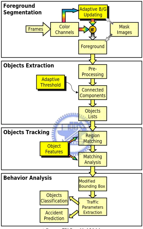
(20) Chapter 3 Multi-objects Tracking System with Adaptive Background Reconstruction In this chapter, we will present our system structure and the details of proposed algorithms. The system structure is composed of four sub-systems: foreground segmentation, objects extraction, objects tracking and behavior analysis. In section 3.1, we use a diagram of the global system to show four sub-systems and their key modules. In section 3.2, we present foreground segmentation’s framework and the adaptive background reconstruction technique. In section 3.3, we present the approach and algorithms of objects extraction. In section 3.4, we present the framework of objects tracking and its relevant algorithms. In section 3.5, we present the behavior analysis module and the analyzing algorithms.. 3.1 System Overview At first, foreground segmentation module directly uses the raw data of surveillance video as inputs. This sub-system also updates background image and applies segmenting algorithm to extract the foreground image. Next, the foreground image will be processed with morphological operation and connected components method to extract individual objects. At the same time, object-based features are also extracted from the image with extracted objects. Main work of the third sub-system is to track objects. The tracking algorithm will use significant object features and input them into analyzing process to find the optimal matching between previous objects and current objects. The occlusion situation and other interaction of moving objects are also handled well in this sub-system. After moving objects are tracked successfully in this sub-system, the consistent labels are assigned to the correct objects. Finally, objects behavior is analyzed and recognized. Useful traffic parameters are extracted and shown in the user interface. The diagram of global system is shown in Fig. 1. 11.

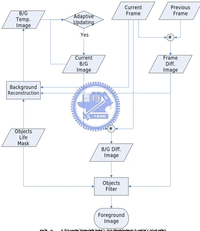
(21) Foreground Segmentation. Adaptive B/G Updating Color Channels. Frames. －. Mask Images. Foreground. Objects Extraction. PreProcessing. Adaptive Threshold. Connected Components Objects Lists. Objects Tracking. Region Matching. Object Features. Matching Analysis. Behavior Analysis. Modified Bounding Box. Objects Classification. Traffic Parameters Extraction. Accident Prediction Fig. 1. Global system diagram. 3.2 Foreground Segmentation The purpose of first sub-system is to extract foreground image. At first, we input the raw data of surveillance video obtained from stationary video cameras to this module. And, the 12.

(22) main processes of this sub-system are foreground segmentation and background reconstruction. In regard to segmentation, there are three basic techniques: 1) frame differencing, 2) background subtraction, and 3) optical flow. Frame differencing will easily produce some small regions that are difficult to separate from noise when the objects are not sufficiently textured. Optical flow’s computations are very intensive and difficult to realize in real time. In [10], a probabilistic approach to segmentation is presented. They used the expectation maximization (EM) method to classify each pixel as moving object, shadow or background. In [31], Kumar proposed a background subtraction technique to segment the moving objects from image sequences. And, the background pixels were modeled with a single Gaussian distribution. In [17], Gupte used a self-adaptive background subtraction method for segmentation. In almost surveillance condition, the video camera is fixed and the background can be regarded as stationary image, so the background subtraction method is the simplest way to segment moving objects. That’s why we adopt this method as the basis of our segmentation algorithm. Besides, the results of frame differencing and previous objects condition are also used in order to achieve the segmentation more reliably. The process of foreground segmentation and background reconstruction is shown in Fig. 2.. 3.2.1 Background Initialization Before segmenting foreground from the image sequences, the system needs to construct the initial background image for further process. The basic idea of finding the background pixel is the high appearing probability of background. During a continuous duration of surveillance video, the level of each pixel appeared most frequently is almost its background level. According to this concept, there are some approaches to find out background image, such as classify and cluster method and Least-Median-Squares (LMedS) method. We use a simpler method that if a pixel’s value is within a criterion for several consecutive frames, it. 13.

(23) means the probability of appearing of this value is high locally or this value is locally stable. This value is regarded as the background value of this pixel. Then the pixel value in background buffer is duplicated to the corresponding pixel in the initial background image.. B/G Temp. Image. Current Frame. Adaptive Updating. Previous Frame. Yes. －. Current B/G Image. Frame Diff. Image. Background Reconstruction. －. Objects Life Mask. B/G Diff. Image. Objects Filter. Foreground Image. Fig. 2. The process diagram of foreground segmentation. This method can build an initial background image automatically even though there are objects moving inside the view of camera during the duration of initialization. The. 14.

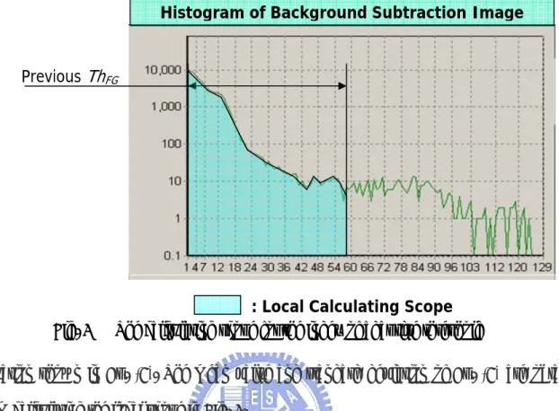
(24) establishing equation is Eq. (1), (2) and (3). In these equations, the superscript C means different color channels. In our segmentation algorithm, we use R, G and intensity channels for background subtraction process. Hit(i,j) records the times of one same value appeared consecutively at pixel(i,j) and Thappear is the threshold of the appearing times. The σBG is a preset variance as the criterion for checking that the current value is the same as the one of buffer image. ⎧ ⎪ Hit (i, j ) + 1, if Hit (i, j ) = ⎨ ⎪1, otherwise ⎩. C3. ∑ ( BG. C =C 1. C buffer. 2⎫ (i, j ) − I C (i, j )) 2 < 3 ∗ σ BG ⎪ ⎬ ⎪ ⎭. (1). C1 ⎧ ( BG buffer (i, j ) * ( Hit (i, j ) − 1) + I C1 (i, j ) ) / Hit (i, j ), ⎫ ⎪⎪ ⎪⎪ C1 BG buffer if Hit (i, j ) > 1 (i , j ) = ⎨ ⎬ ⎪ C1 ⎪ ⎪⎩ I (i, j ), if Hit (i, j ) ≤ 1 ⎪⎭. (2). C1 BG C1 (i, j ) = BG buffer (i, j ),. (3). if. Hit (i, j ) ≥ Thappear. 3.2.2 Adaptive Background Updating We introduce an adaptive threshold for foreground segmentation. The adaptive threshold includes two parts: one is a basic value and the other is adaptive value. And, we use the equation shown in Eq. (4) to produce the threshold. The two statistic data (Peaklocal, STDEVlocal) are calculated in the specific scope as shown in Fig. 3. This adaptive threshold will assist the background updating algorithm in coping with environmental changes and noise effects. Th FG = Valuebasic + 1.5 * Peak local + STDEVlocal. (4). At outdoor environment there are some situations that result in wrong segmenting easily. Those situations include waving of tree leaves, light gradual variation and etc. Even there are sudden light changes happened when the clouds cover the sun for a while or the sun is revealed from clouds. We propose an adaptive background updating framework to cope with. 15.

(25) those unfavorable situations. Firstly, we introduce a statistic index which is calculated by the Histogram of Background Subtraction Image. Previous ThFG. Fig. 3. : Local Calculating Scope The calculating scope for the index of adaptive threshold. equation shown in Eq. (5). The mean value and standard deviation of Eq. (5) are obtained from calculating the local scope in Fig. 3. Index = Meanslocal + 3 ∗ STDEVlocal. (5). According to this index, we adjust the frequency of updating the current background image adaptively and the updating frequency is defined as several phases. The background updating speed will increase or decrease with the updating frequency. Besides, the final phase is an extra heavy phase which is designed for those severely sudden change conditions. At this phase, the background image will be updated directly. These phases and their relevant parameters are listed in Tab. 1. Tab. 1. Phases of adaptive background updating. Phase. Condition. Sampling rate. Freq in Eq.(8). Normal. Index < 12. 1/30. 30. Middle I. 12 ≤ Index < 18. 1/24. 24. Middle II. 18 ≤ Index < 24. 1/16. 16. 16.

(26) Heavy I. 24 ≤ Index < 30. 1/8. 8. Heavy II. 30 ≤ Index < 36. 1/4. 4. Extra Heavy. 36 ≤ Index. Directly update. N/A. At the reconstruction process, the temporary background image is the result of current frame image filtered by a background mask image. The background mask image is updated based on frame differencing image and objects life mask image. Its updating equation is shown in Eg. (6). Then the current background image will be updated with itself and temporary background image by the equation in Eq. (7) & (8). The parameter α is a weighting factor and the ThDiff is a threshold for frame differencing. The parameter Freq is the updating frequency and results from the adaptive background updating algorithm. ⎧⎪255, if Diff Frame (i, j ) < Th Diff I Life(i, j ) ≤ Th M _ life Mask BG (i, j ) = ⎨ ⎪⎩0, elsewise. ⎫⎪ ⎬ ⎪⎭. ⎧ I (i, j ), if Mask BG (i, j ) = 255⎫ BG temp (i, j ) = ⎨ ⎬ ⎭ ⎩ BG (i, j ), Otherwise. ⎧⎪α * BG temp (i, j ) + (1 − α ) * BG (i, j ), if Index frame % Freq = 0 BG (i, j ) = ⎨ ⎪⎩ BG (i, j ), Otherwise. (6). (7). ⎫⎪ ⎬ ⎪⎭. (8). 3.2.3 Background Subtraction As mentioned in section 3.2, we use the background subtraction method to segment foreground image. We use R, G and intensity channels to perform the subtraction and the intensity channel is calculated by the equation shown in Eq. (9). The computation loading, blue channel’s sensitivity to the shadow and the characteristics of traffic intersections are the main reasons why those channels are introduced by our framework. Then the background subtraction image is obtained by combining three channels’ subtraction directly as shown in. 17.

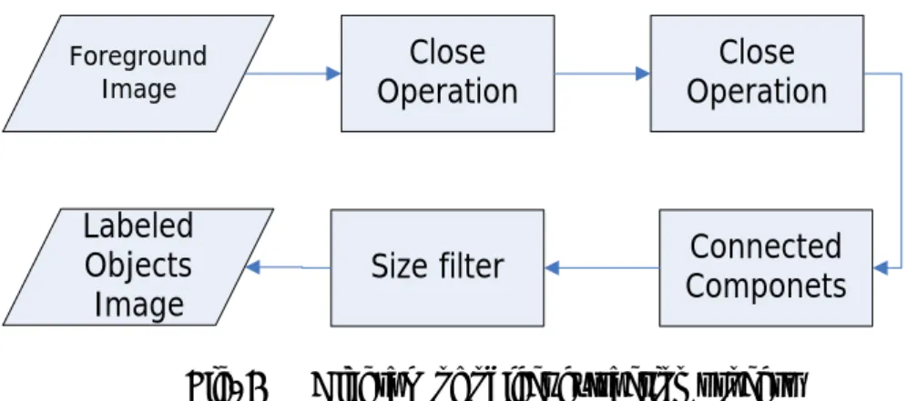
(27) Eq. (10). I I (i, j ) = (77 * I R (i, j ) + 151 * I G (i, j ) + 28 * I B (i, j )) / 256. (9). Diff BG (i, j ) = ( I I (i, j ) − BG I (i, j ) + I R (i, j ) − BG R (i, j ) + I G (i, j ) − BG G (i, j ) ) / 3 (10) Next, the background subtraction image is filtered by a foreground mask image. This mask image consists of previous extracted objects with their life information and frame temporal differencing image. The frame temporal differencing is considered only with the intensity channel and showed in Eq. (11). The objects life mask image is based on the appearing period of each object. We assign the value of its life feature to those pixels which this object belongs to. We can use the equation Eq. (12) to obtain the foreground mask. This mask can filter out some noise or ghost regions that we don’t desire to extract. As shown in Eq. (13), after applying the foreground mask to background subtraction image, we can get the foreground image and it’s the output of this sub-system. Diff Frame (i, j ) = I nI (i, j ) − I nI −1 (i, j ). (11). ⎧⎪0, if Diff Frame (i, j ) < ThDiff I Life(i, j ) ≤ 0 Mask FG (i, j ) = ⎨ ⎪⎩255, elsewise ⎧ Diff BG (i, j ), if Mask FG (i, j ) = 255 ⎫ FG (i, j ) = ⎨ ⎬ ⎩0, otherwise ⎭. ⎫⎪ ⎬ ⎪⎭. (12). (13). 3.3 Objects Extraction In this sub-system, we will use the connected components algorithm to extract each object and assign it a specific label to let the system recognize different objects easily. Before the process of connected components algorithm, we will apply morphological operation to improve the robustness of object extraction. The result of the connected components algorithm is the labeled objects image. The process of this sub-system is shown in Fig. 4.. 18.

(28) Foreground Image. Labeled Objects Image. Fig. 4. Close Operation. Close Operation. Size filter. Connected Componets. Diagram of object extraction process. Then we will build a current objects list with their basic features such as position, size and color according to the labeled objects image. We use a spatial filter and a B/G check filter to remove ghost objects or objects at the boundaries. We also calculate the overlap area between current objects list and previous objects list. If the overlap area is larger than the threshold, a region relation will be established. This process’s diagram is shown in Fig. 5. The current objects list and region relation list will pass to tracking module for further process.. Yes Overlap Relation List. Labeled Objects Image. Spatial Filter. B/G Check Filter. > Thoverlap. Overlap Area. Current Objects List. No Next P. Object. Previous Objects List. Yes. No. Fig. 5. Diagram of establishing objects list. 3.3.1 Pre-Processing Before the process of connected components algorithm, we apply some pre-processing to smooth the contours of objects and remove the noise. Our algorithm uses closing process. 19.

(29) twice and this closing operation can help fill the holes inside the object regions. The morphological operation closing consists of the dilation process and the erosion process and the performing order of these two processes is important. Dilation-erosion is the closing operation but erosion-dilation is the opening operation. After the process of the closing operation, we apply the adaptive threshold of foreground segmentation to the result images and then extract moving objects by the connected component algorithm.. 3.3.2 Connected Components Algorithm Each object in the foreground image must be extracted and assigned a specific label for further processes. The connected components algorithm [40], [41] is frequently used to achieve this work. Connectivity is a key parameter of this algorithm. There are 4, 8, 6, 10, 18, and 26 for connectivity. 4 and 8 are for 2D application and the others are for 3D application. We used the 8-connectivity for our implementation. The connected component algorithm worked by scanning an image, pixel-by-pixel (from top to bottom and left to right) in order to identify connected pixel regions. The operator of connected components algorithm scanned the image by moving along a row until it came to a point (p) whose value was larger than the preset threshold of extraction. When this was true, according to the connectivity it examined p’s neighbors which had already been encountered in the scan. Based on this information, the. labeling of p occurred as follows. If all the neighbors were zero, the algorithm assigned a new label to p. If only one neighbor had been labeled, the algorithm assigned its label to p and if more of the neighbors had been labeled, it assigned one of the labels to p and made a note of the equivalences. After completing the scan, the equivalent label pairs were sorted into equivalence classes and a unique label was assigned to each class. As a final step, a second scan was made through the image, during which each label was replaced by the label assigned to its equivalence classes. Once all groups had been determined, each pixel was labeled with a graylevel or a color (color labeling) according to the component it was assigned to.. 20.

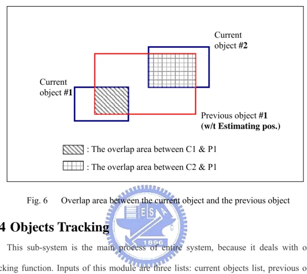
(30) Next, we use a predefined threshold of object size to filter out some large noise and ghost regions. After applying size filter, we can get the labeled objects image. In this image, the different gray level presents different object so we can gather the pixels with same gray level to form the region of a specific object.. 3.3.3 Objects List When building objects list, we apply two filters to remove some unwanted objects. Firstly, spatial filter will remove those objects near boundaries with a preset distance. This can solve the tracking confusion by partial appearance on boundaries when objects are just leaving or entering the field of view (FoV). This filter can be extended its area of filtering to become a scene mask for simplifying the effective region of the FoV. Secondly, the B/G check filter is a combination of three Sobel operations. We use first Sobel operation to find the edges of each object. Then the second Sobel operation is performed with the current frame on all the edge pixels which were obtained from first Sobel operation. The third Sobel operation is performed with the background image on the same edge pixels. We mark the pixels if the value of their third Sobel operation is bigger than the value of second Sobel operation. Finally, we use a preset threshold for the ratio of marked pixels to all edge pixels to judge whether this object is a background ghost object. When establishing objects list, we also extract three basic categories. They are central position, size of bounding box and YCbCr color information. At the same time, we calculate the overlap area between each current object and previous object based on the estimated position. We use the size of bounding box and central position as input data and a simple method to calculate the size of overlap area that is shown in Fig. 6. Then we calculate the ratio of the overlap area to the minimum area of two objects by Eq. (14). Ratiooverlap = Areaoverlap / Min( Areacurrent _ obj . , Area previous _ obj ). (14). If the overlap ratio is larger than a preset threshold, one relation of this current object and. 21.

(31) the previous object is established. This overlap relation list is an important reference list for objects tracking sub-system.. Current object #2. Current object #1 Previous object #1 (w/t Estimating pos.) : The overlap area between C1 & P1 : The overlap area between C2 & P1. Fig. 6. Overlap area between the current object and the previous object. 3.4 Objects Tracking This sub-system is the main process of entire system, because it deals with objects tracking function. Inputs of this module are three lists: current objects list, previous objects list and overlap relation list. This sub-system can analyze the relation between current objects and previous objects and obtain other properties of objects, such as velocity, life, trajectory and etc. The tracking framework can be divided into several modules and we will present each module and introduce its algorithm. The diagram of tracking process is shown in Fig. 7. The overlap relation list will be simplified by some constraint and rules. In [42], Masound used an undirected bipartite graph to present relations among objects and apply a parent structure constraint to simplify the graph computation. The constraint is equivalent to saying that from one frame to the next, an object may not participate in a splitting and a merging at the same time. We use the similar thought of decreasing the computation of overlap relation but the simplifying algorithm is more compact and effective. After. 22.

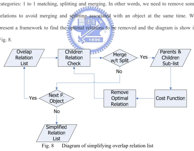
(32) simplifying overlap relation list, the remaining relations can be classified into three categories: 1 to 1 matching, splitting and merging.. Fig. 7. Diagram of tracking process. 23.

(33) Besides, those objects without relevant overlap relations belong to objects appearing or objects disappearing categories. According to the characteristics of different categories, we apply further matching and analyzing algorithms with proper features to track objects accurately. Extended scope matching process and isolated objects process help track the objects that can’t meet matching equation of those relation categories. Finally, all current objects are tracked and assigned their correct label and status. This tracked objects list is the input of behavior analysis sub-system and forms the previous objects list in next frame’s process.. 3.4.1 Matching Analysis Firstly, we need a simplifying relations process to let those relations limit to three categories: 1 to 1 matching, splitting and merging. In other words, we need to remove some relations to avoid merging and splitting associated with an object at the same time. We present a framework to find the optimal relations to be removed and the diagram is show in Fig. 8.. Fig. 8. Diagram of simplifying overlap relation list. The cost function consists of overlap area ratio and difference area ratio to find out the optimal one. Instead of finding all possible removing combination, we use the cost function to. 24.

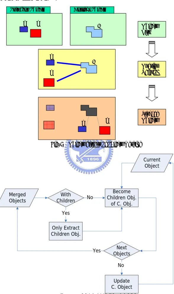
(34) find one optimal relation to be removed at each evaluating cycle and run this process as a recursive process until the violation doesn’t exist. The equations for the evaluation are shown in Eq. (15) and (16). If cost of the first optimal candidate and cost of the second one are similar within a threshold and we will choose the optimal relation depending on their effectiveness of eliminating the violation. Ratio Diff = Area curr. − Area pre. / Max ( Area curr. , Area pre. ). (15). Cost = RatioDiff / Ratiooverlap. (16). After simplifying overlap relation list, the matching analysis can be separated into three processes. First process is 1 to 1 matching. This is a quite simple process of matching analysis and we only apply a matching equation Eq. (17) to confirm this matching. Then remaining work is only to update object’s features: label, type, status, velocity, life, child objects and trajectory. The other two processes are presented in 3.4.2 & 3.4.3 section.. Match1 _ to _ 1. ⎧ Area pre. − 1 < Th1 _ to _ 1 ⎪1, if Area curr. =⎨ ⎪0, Otherwise ⎩. ⎫ ⎪ ⎬ ⎪ ⎭. (17). 3.4.2 Objects Merging When multiple previous objects associated with one current object according to the overlap relation list, an objects merging event happened. The objects history of objects merging is shown in Fig. 9. During the process of objects merging, the main work is to reconstruct the parent-children association. We use the property of children list to present the objects which were merged into the parent object and those objects in children list keep their own properties. If the previous object is with children, we only append the children of this previous object to current object’s children list. After appending all objects or their children, the current object becomes a group of those merged objects, like a parent object. The diagram of objects. 25.

(35) merging is shown in Fig. 10. Previous objects i. Current objects. j. 1. i. Objects List. 1. Overlap Relation. j. Tracked Objects. j. i. Fig. 9 Objects history of objects merging Current Object. Merged Objects. With Children. No. Become Children Obj. of C. Obj.. Yes Only Extract Children Obj. Yes. Next Objects No Update C. Object. Fig. 10 Diagram of objects merging. 26.

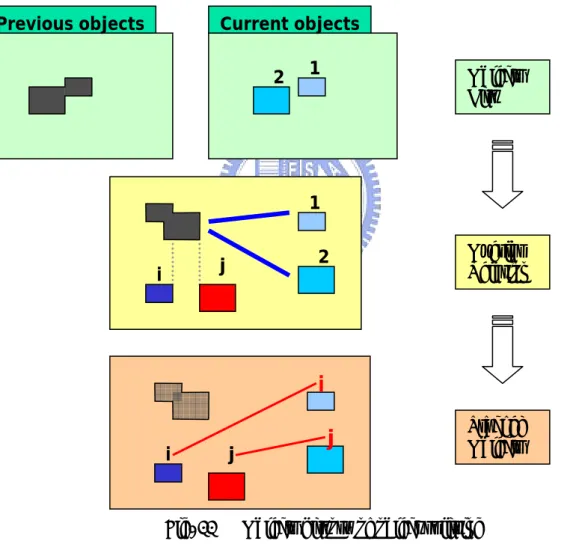
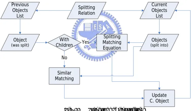
(36) 3.4.3 Objects Splitting The most complicated process of tracking analysis is object splitting. It happens when a single previous object associated with multiple current objects. The splitting case is similar with the inversion of merging case and its objects history is shown in Fig. 11. Splitting events often result from occlusion and objects merging event is one situation of occlusion. As some research’s definitions, there are two kinds of occlusions and one is explicit occlusion and another is implicit occlusion. In brief, explicit occlusion happens inside FoV and implicit occlusion happens outside FoV. Previous objects. Current objects 2. 1. Objects List. 1 2. j. i. Overlap Relation. i i. Fig. 11. j. j. Tracked Objects. Objects history of object splitting. Our algorithm deals with these occlusions by the property of children list. If the previous object doesn’t have the child object, this splitting results from implicit occlusion. If the quantity of previous object’s children objects is less than quantity of split objects, this splitting is a partial splitting case. And if the previous objects are with explicit occlusion and. 27.

(37) its children are as many as split objects, this will be a fully splitting. The process of object splitting is shown in Fig. 12. In this process, we check the status of children objects of the previous object firstly. If none of children object, we do a similar matching process to assign the label of the previous object to the most similar object among these current objects and the others keep unmatched status. If the object has children objects, we will apply the matching algorithm to find the optimal matching between children objects of the previous object and the current objects. The algorithm is based on object’s position, size and color. We use three preset thresholds to filter the matching candidates in advance and use the feature of object’s position to find the optimal matching. After matching successfully, we update the matched objects’ properties. Previous Objects List. Object (was split). Current Objects List. Splitting Relation. With Children. Splitting Matching Equation. Yes. Objects (split into). No Similar Matching Update C. Object. Fig. 12. Process of object splitting. 3.4.4 Other Matching Processes After three matching process presented in previous sections, there are still some objects unmatched. Those objects belong to not only previous objects but also current objects. Main causes of those unmatched objects are new objects appeared or old objects had left out of FoV. Besides the two main causes, previous objects unmatched sometimes result from occlusion by background or long movement between frames. And, possible reasons of current objects. 28.

(38) unmatched are split from implicit occlusion, revelation from background occlusion or exceeding the thresholds when previous matching. Our algorithm presents two additional processes to deal with those situations. One is extended scope matching and its diagram is shown in Fig. 13. In this process, we search unmatched current objects inside a preset scope of each unmatched previous object and use a matching function to match them. The matching function depends on the object’s size and color features and it should be within the thresholds. Previous Objects List. Unmatched Object. With One Child. Unmatched Objects. Current Objects List. Extended scope Matching. Update C. Object. No. Yes Replace with the child. Fig. 13. Process of extended scope matching. The other process is isolated objects process. Unmatched previous objects will keep their all properties except life and position. Their life feature will be decreased and their position will be updated with their estimating position. Then these unmatched previous objects will be duplicated into the current objects list. Finally, unmatched current objects will be regarded as new objects and be assigned with new labels. The diagram of this process is shown in Fig. 14.. Fig. 14. Diagram of isolated objects process 29.

(39) 3.4.5 Current Objects List Updating After the objects are tracked, the current objects list also is updated with matching information. In this section, we introduce those updating rules and the status of object’s properties. The updating descriptions of these properties are listed below: Position: observed value, needn’t to be updated. Size: observed value, needn’t to be updated. Color: observed value, needn’t to be updated. Status: depends on the tracking analysis. Children List: depends on the tracking analysis. Label: if matched, follow matched previous object’s value. If not, it will be assigned a. new label. Life: presents in 3.4.6 section. Type: if matched, follow matched previous object’s value. Trajectory: uses matched previous object’s data and current object’s position data. Velocity:. if trajectory’s points are less than five points, we use an adaptive equation Eq.. (18) to calculate its velocity. Otherwise, a line-fitting algorithm is applied to find a fitting velocity. Vx = β ∗ Vx previous + (1 − β ) ∗ ( X current − X previous ) Vy = β ∗ Vy previous + (1 − β ) ∗ (Ycurrent − Y previous ). (18). Estimated Position: use the velocity to estimate the position for next frame.. 3.4.6 Life and Status of Objects In order to assist tracking framework, our algorithm exploits the temporal information and create a life feature for this purpose. Fig. 15 shows the diagram of the life feature. We use the life feature to define the status of objects. The threshold of life feature can help filter out some ghost objects which usually appear and disappear very quickly. And, this. 30.

(40) threshold also defines the dead phase for filtering out those objects that can’t be tracked anymore for a period time. The other threshold of appearing is used to confirm that the object is valid and our behavior analysis module will not deal with the invalid objects. The life feature will be updated with the matching results. If there is no matching, the life feature will be decreased by one as a degeneration phase. Otherwise, with a successful matching the life feature will be increased by one as a growth phase. New. Next Frame. Matching. Yes. No Degeneration ( Life-- ). Growth ( Life++ ). No Dead. Yes. Life < Thlife. Hide. No. Life > Thappear Yes. Appear. Fig. 15. Diagram of life feature. We also design another type of life feature for the stopped objects. This sleep_life feature records the consecutive duration of an object which has stopped. If the sleep_life feature of an object is larger than a preset threshold, this object will become dead immediately and its region will be duplicated into background image at the same time. The update equation is shown in Eq. (19). According to the scene characteristics, we can setup this threshold to provide optimal control of stopped objects. BG (i, j ) = I current (i, j ), (i, j ) ∈ pixels of Obj. m, if Sleep _ life( m) > Thsleep _ life (19). 31.

(41) 3.5 Behavior Analysis The main purpose of this sub-system is to analyze the behavior of moving objects to extract traffic parameters. In this sub-system, we introduce several modules to deal with high level objects features and output real-time information related with traffic parameters, such as objects classification and accident prediction. The diagram of this process is shown in Fig. 16. Tracked Objects List. Modified Bounding Box. Objects Classification. Monitoring UI. Accident Prediction. Fig. 16. Diagram of behavior analysis. We present a modified bounding box method and it can give a much tighter fit than the conventional bounding box method. The direction of the modified bounding box’s principle axis is same as the velocity vector of this object. We created eight bounding lines in the principle direction and its perpendicular direction at four points of object’s limit. Then we choose the outer ones of these bounding lines as the boundaries of the modified bounding box of this object. This method is a really simple and effective method to fit the vehicle’s shape. Its diagram is shown in Fig. 17.. 3.5.1 Camera Calibration and Object Classification Camera calibration is an important process if we want to extract spatial information or other information related with the locations. We introduce a simple method to perform the function of camera calibration and the equations of this method are shown in Eq. (20) and (21). This is a two-dimension calibration method and can compensate the dimensional distortion which results from different location at camera view.. 32.

(42) The limits of objects. Modified bounding box. The limits of objects. Traditional bounding box. Perpendicular vector Velocity vector. Fig. 17. Diagram of modified bounding box. Before we apply the camera calibration to our system we need several data to calculate the calibrating matrix M in advance. We use the dimensions and the locations of some moving objects to calculate the matrix M. Besides, in order to simplify the computation of the camera calibration, we normalized those properties such as width, height and velocity to the calibrated values of central position of the image. The equation of normalization is shown in Eq. (22) and the reference value is obtained by the Eq. (20) with the central position of the images. ⎡ Xi ⎤ ⎡ Xw⎤ ⎢ ⎥ ⎢Yw ⎥ = M calibration ⎢Yi ⎥ ⎣ ⎦ ⎢⎣1 ⎥⎦ ⎡p M calibration = ⎢ 11 ⎣ p21. ref center. p12 p22. (20). p13 ⎤ p23 ⎥⎦. (21). ⎡ Pximage _ center ⎤ ⎢ ⎥ = M calibration * ⎢ Pyimage _ center ⎥ ⎢1 ⎥ ⎣ ⎦. Featurecalibrated. ⎡ Px ⎤ = Featureoriginal * ref center /( M calibration * ⎢ Py ⎥ ) ⎢ ⎥ ⎢⎣1 ⎥⎦. 33. (22).

(43) With camera calibration, we can process object classification based on preset criteria of object’s size and velocity easily. In brief, we use the calibrated feature of size to classify moving objects into large cars, cars, motorcycles and people. Because the size of motorcycles is similar with the one of people, we classify motorcycles and people again according to the velocity feature additionally. The rule of classifying is shown in Table 2. Table 2. Rule of objects classification. Object type. Drawing color. Size. Velocity. People. Red. Size < SizeMotor. Vel. < VelMotor. Motorcycles. Yellow. Size < SizeCar. N/A. Cars. Blue. SizeCar< Size <SizeL.car. N/A. Large Cars. Green. Size > SizeL.car. N/A. 3.5.2 Accident Prediction We also present a prediction module for traffic accidents. We analyze the trajectories of any two objects and classify the relation of the objects into four types: both stopped objects, only one moving object, same moving direction and different moving directions. The equations of classifying are shown in Eq. (23). The prediction module only processed the later three types. ⎧0. ( Both stopped ), if V 1 = 0 I V 2 = 0 ⎫ ⎪ I . (Only one moving ), if (V 1 = 0 I V 2 ≠ 0) U (V 1 ≠ 0 I V 2 = 0) ⎪ ⎪ ⎪ Type = ⎨ ⎬ ⎪ II .( Same dir.), if V 1 ≠ 0 I V 2 ≠ 0 I Vx1 * Vy 2 − Vy1 *Vx 2 = 0 ⎪ ⎪⎩ III . ( Different dir.), otherwise ⎪⎭. (23). Firstly, for the type I, the closest position is calculated and the distance between these two objects in that position is compared with a preset threshold to predict the occurrence of an accident. The diagram of this type is shown in Fig. 18.. 34.

(44) Vtemp Distclosest Objectstopped Objectmoving Vmoving. Positionclosest Fig. 18. Diagram of type I of the relation of two objects. The equations of the closest position and the distance are shown in Eq. (24) and (25). Then we use the equation in Eq. (26) to predict the occurrence of accidents and the occurring position. 2. 2. Tclosest = (Vy mov . ∗ ( Py stopped − Py mov . ) + Vxmov . * ( Px stopped − Pxmov . )) /(Vx mov . + Vy mov . ) 2. Vxtemp = −Vymov . , Vytemp = Vxmov . , Vtemp = Vxmov . + Vymov .. (24). 2 2. 2. Ttemp = (Vxmov . ∗ ( Py mov . − Py stopped ) − Vy mov . * ( Pymov . − Py stopped )) /(Vxmov . + Vymov . ). (25). Distclosest = Vtemp * Ttemp . ⎧T , if Tcloest > 0 I Dist cloest < Dist accident ⎫ Tclosest = ⎨ cloest ⎬ ⎩ No accident , otherwise ⎭ Px accident = Tclosest * Vx mov . + Px mov .. (26). Py accident = Tclosest * Vy mov . + Py mov .. Secondly, we analyze the type of same moving direction further and only focus on the situation in which trajectories of the two objects are almost on the same line. The equation Eq. (27) is used for checking whether the trajectories are almost on the same line with a threshold. Then the occurrence of accidents and the occurring position are predicted by the equations shown in Eq. (28). This type’s diagram is shown in Fig. 19.. 35.

(45) Object #1. Object #2. V1. Fig. 19. V2. Diagram of type II of the relation of two objects. ⎧ At the same line, if Vx1 * ( Py 2 − Py1) − Vy1 * ( Px 2 − Px1) < Thsame _ line ⎫ Type = ⎨ ⎬ ⎩ Parallel , otherwise ⎭. (27). Tsame _ line = ( Px1 − Px 2) /(Vx 2 − Vx1) − Distaccident / Vx 2 − Vx1 ⎧Tsame _ line , if Tsame _ line > 0⎫ Tsame _ line = ⎨ ⎬ ⎩ No accident , otherwise ⎭. (28). Pxaccident = Tsame _ line * Vx1 + Px1 Py accident = Tsame _ line * Vy1 + Px1. Thirdly, if the moving directions of two objects are different, we use the equations shown in Eq. (29) to obtain the time for objects reaching the crossing of their trajectories. Then we can predict the occurrence of accidents by the equation Eq. (30) and obtain the occurring position. This type’s diagram is shown in Fig. 20. Δ = Vx 2 * Vy1 − Vx1 * Vy 2 T 1 = (Vx 2 ∗ ( Py 2 − Py1) + Vy 2 * ( Px 2 − Px1)) / Δ T 2 = (Vx1 ∗ ( Py 2 − Py1) − Vy1 * ( Px 2 − Px1)) / Δ. (29). 1 1 ⎫ 1 ⎧ )⎪ ⎪T 1, T 2, if T 1 > 0 I T 2 > 0 I T 1 − T 2 < ( Distaccident ) * ( + T 1, T 2 = ⎨ 2 V1 V 2 ⎬ ⎪⎭ ⎪⎩ No accident , otherwise Pxaccient = T 1 * Vx1 + Px1 Py accidnt = T 1 * Vy1 + Py1. 36. (30).

(46) V1. Object #1. Object #2 V2 Fig. 20. Diagram of type III of the relation of two objects. 37.

(47) Chapter 4 Experimental Results We implemented our tracking system with PC system and the equipment of this PC is Intel P4 2.4G and 512MB RAM. The software we used is Borland C++ Builder 6.0 on Window 2000 OS. The inputs are video files (AVI uncompressed format) or image sequences (BMP format) and all the inputs are in the format of 320 by 240. These inputs were captured by ourselves with a DV at traffic intersection or referred to testing samples which were used by other research. In the section 4.1, we will show the experimental results of background reconstruction and foreground segmentation. In section 4.2, the results of objects tracking will be represented. In section 4.3, the implemented system will be presented and the results of extraction of traffic parameters are also demonstrated.. 4.1 Results of Background Reconstruction and Foreground Segmentation 4.1.1 Background Initialization We use a video file which was captured at traffic intersection to present our proposed algorithm for background initialization. The threshold of appearing is preset as 15 and the duration of initializing is 200 frames. As the result, there are 76416 pixels which had fully updated and the updated ratio is 99.5%. Those partial updated pixels only account for 0.5% and will be updated soon by background reconstruction module.. 38.

(48) (a): Frame #1. (b): Frame #6. (c): Frame #16. (d): Frame #26. (e): Frame #36. (f): Frame: #46. (g): Frame #66. (h): Frame #86. 39.

(49) Fig. 21. (i): Frame #86 (j): Frame # 166 Temporary background images during background initialization. Some temporary background images which were created during background initialization are shown in Fig. 21. We can find that moving objects which can be removed automatically by our initializing algorithm in images (a) ~ (h). The images (i) and (j) are locally enlarged images and there are some small regions which hadn’t been updated in image (i). Then those regions had been updated well in image (j). This is the reason why the duration of initialization that is preset as 200 frames and we intend to construct robust initial background image.. 4.1.2 Adaptive Background Updating The main purpose of background updating module is to reconstruct a robust background image. But there are some situations that result in wrong background images easily at outdoor environment. We use the datasets of PETS (Performance Evaluation of Tracking and Surveillance) to perform the adaptive background updating algorithm. The video is PETS2001 [43] dataset2 training video and it’s prepared for its significant lighting variation. We also performed the tracking on this video using fixed background updating method with two different updating frequencies in order to compare with our proposed algorithm. The experimental results are shown in Fig. 22 and the #XXXX–a images show the results using our adaptive updating algorithm. The leading number means the index of image sequences. The upper images are images of results of background subtraction and the lower. 40.