金屬消能制震板之理論分析與實驗

(1)

國立交通大學

土木工程學系碩士班

碩士論文

金屬消能制震板之理論分析與實驗

A Theoretical and Experimental Study of Metallic Yielding Damper

研究生：林峻毅

指導教授：王彥博博士

李建良博士

(2)

A Theoretical and Experimental Study of Metallic Yielding Damper

研究生：林峻毅 Student: Chun-Yi Lin

指導教授：王彥博博士 Advisor: Dr. Yen-Po Wang

李建良博士 Dr. Chien-Liang Lee

國立交通大學

土木工程學系

碩士論文

A Thesis

Submitted to Department of Civil Engineering

College of Engineering

National Chiao Tung University

in partial Fulfillment of the Requirements

for the Degree of

Master

in

Civil Engineering

June 2004

Hsinchu, Taiwan, Republic of China

(3)

博碩士論文授權書

（國科會科學技術資料中心版本，93.2.6）

本授權書所授權之論文為本人在交通大學 (學院) 土木工程系所

結構組九十二學年度第二學期取得碩士學位之論文。

論文名稱：金屬消能制震板之理論分析與實驗

; 同意不同意

本人具有著作財產權之論文全文資料，授予行政院國家科學委員會科學技術資料中心(或其改制後之機構)、國家圖書館及本人畢業學校圖書館，得不限地域、時間與次數以微縮、光碟或數位化等各種方式重製後散布發行或上載網路。本論文為本人向經濟部智慧財產局申請專利（未申請者本條款請不予理會）的附件之一，申請文號為：＿＿＿＿＿＿，註明文號者請將全文資料延後半年後再公開。

;同意不同意

本人具有著作財產權之論文全文資料，授予教育部指定送繳之圖書館及本人畢業學校圖書館，為學術研究之目的以各種方法重製，或為上述目的再授權他人以各種方法重製，不限地域與時間，惟每人以一份為限。上述授權內容均無須訂立讓與及授權契約書。依本授權之發行權為非專屬性發行權利。依本授權所為之收錄、重製、發行及學術研發利用均為無償。上述同意與不同意之欄位若未鉤選，本人同意視同授權。

指導教授姓名：王彥博教授

研究生簽名：學號：9116503

（親筆正楷）（務必填寫）

日期：民國

93 年 6 月 30 日

1. 本授權書 (得自 http://sticnet.stic.gov.tw/sticweb/html/theses/authorize.html 下載或至 http://www.stic.gov.tw 首頁右下方下載) 請以黑筆撰寫並影印裝訂於書名頁之次頁。 2. 授權第一項者，請確認學校是否代收，若無者，請個別再寄論文一本至台北市 (106) 和平東路二段106 號 1702 室國科會科學技術資料中心黃善平小姐。（電話：02-27377606 傳真：02-27377689）

(4)

- ii -

金屬消能制震板之理論分析與實驗

學生：林峻毅指導教授：王彥博博士

李建良博士

國立交通大學土木工程研究所

摘要

現代結構防震設計的目標在於各種強度不同的地震之下，結構物仍可保有其性能而使內部之功能正常運作。為達到此一目的，傳統一味增加結構元件尺寸的作法已被秉棄，取而代之的是在結構系統之中加進消能減震元件、控制系統或是隔震系統。金屬消能制震板的基礎力學理論包含勁度、降伏位移、降伏荷載之計算，以及設計上的細節考量；實尺寸以及縮小尺寸之制震板的元件測試結果，將用於驗證這些理論的正確性。本文提出一套可行的方法，在不裝設荷重元之情況下，藉由制震板上貼附應變計量得之應變，配合Ramberg-Osgood 遲滯模型，推估制震板所受之彎矩與剪力。為解決數值計算上之困難，並將計算流程程式化，本文推導出Ramberg-Osgood 遲滯模型之另一種表示方程式，且提出相關之查表法。實驗結果證實藉由本文提出之方法，吾人可得合理之預測結果。制震板之耐震性試驗藉由一系列之振動台試驗進行，制震板尺寸遵照先前參數分析結果並配合電腦模擬進行設計，目標在於同時降低一座五層樓鋼構架模型其在多種不同地震下的加速度與位移反應，實驗結果與電腦數值模擬均顯示制震板可以有效達到其設計目標。關鍵字：消能減震、金屬制震板、遲滯迴圈、Ramberg-Osgood、應變。

(5)

- iii -

A Theoretical and Experimental Study of Metallic Yielding Damper

Student: Chun-Yi Lin Avisors: Dr. Yen-Po Wang

Dr. Chien-Liang Lee

Department of Civil Engineering

National Chiao Tung University

ABSTRACT

To achieve desirable seismic performance, the traditional method of increasing the dimension of structural members is discarded by introducing energy dissipation systems, control systems or seismic isolation systems into the structural design. One of the effective mechanisms available for seismic energy dissipation is through the inelastic deformation of metals.

In this thesis, the fundamentals of metallic yielding damper including determination of stiffness, yielding displacement, yielding loads and design considerations have been introduced. Component tests for both full-scale and scaled-down damper have been conducted. A novel methodology for estimating the moment and shear force from strain with the Ramberg-Osgood Hysteresis model is proposed. To overcome numerical difficulties, an alternative form of the Ramberg-Osgood equations was derived to facility programming. Experimental results show that by the proposed methodology, one may predict the inelastic behavior of the damper with satisfactory accuracy.

Seismic performance test of the damper has also been conducted via a series of shaking table tests. The dimension of the damper was determined, based on preliminary parametric studies via computer simulations by SAP2000, to meet the design goal of suppressing both the acceleration and displacement responses of the structure simultaneously. Results show that the dampers are effective in seismic response control of building structures. Both displacement and acceleration responses can be simultaneously suppressed to a large extent.

Keywords: energy dissipation, metallic yielding damper, hysteresis, strain,

Ramberg-Osgood.

(6)

- iv -

ACKNOWLEDGEMENT

首先最要感謝吾師王彥博教授提供學生一個良好的研究環境，並給

予學生最豐富的指導，使學生具備從事研究工作的基本功夫。此外，吾師

對於學術研究所保有的熱忱與致力於解決工程實務問題的用心，亦為學生

師法的典範。吾師亦常常提供許多新穎的觀念，以增加學生思考的空間，

並且在學生的生涯規劃上提供許多寶貴的建議，在此特向吾師致上最誠摯

的謝意。

論文口試承蒙翁正強教授、黃武龍博士、胡宗和博士、李建良博

士親臨指導，並提供諸多珍貴的意見，使得論文的組織及疏漏之處得以獲

得改進，在此學生亦要表示感激之意。

感謝研究室諸學長鄧敏政博士、廖偉信博士、李建良博士（口試委員

之一），嘉賞學長，同學雅婷、啟晉、逸軒及明坤等於研究上的討論與實

驗上的鼎力協助，使得諸多試驗得以如期完成。此外，感謝同窗學長黃經

理銘峰、鈺文、連杰等於學習過程中的相互勉勵與日常生活中的互動。

最後，謹以本文獻給我最親愛的雙親與弟弟。

謹誌於交大工程二館

2004 年 7 月

(7)

- v -

List of Figures

Fig. 1.1 The earth’s seismicity outlines plate margins ... 2

Fig. 1.2 Classification of structural protective systems... 5

Fig. 1.3 Several metallic yielding devices ... 7

Fig. 1.4 ADAS ... 8

Fig. 1.5 A photo and detailed design of TADAS ... 8

Fig. 1.6 A photo of RADAS ... 8

Fig. 1.7 Pall Friction Device ... 10

Fig. 1.8 A viscoelastic damper ... 11

Fig. 1.9 A Fluid Damper... 12

Fig. 1.10 Buildings installed with TMD... 12

Fig. 2.1 X-shaped metallic yielding damper... 19

Fig. 2.2 Error of neglecting shear deformation on stiffness ... 21

Fig. 2.3 Stiffness ratio

(

k k′_d _d

)

with respect to height-to-thickness ratio

(

h t

)

for various safety factors

( )

SF ... 25

(

k k′d d

)

with respect to height-to-thickness ratio

(

h t

)

for various thicknesses

( )

t ... 25

Fig. 2.5 Yielding displacement with respect to height-to-thickness ratio

(

h t

)

for various thicknesses of the damper ... 27

Fig. 2.6 Height-thickness ratio

(

h t

)

with respect to yielding displacement ratio

(

_{∆ ∆}_y ′_y

)

for various thicknesses of the damper ... 27

Fig. 3.1 Common mathematical models for stress-strain relationship ... 30

Fig. 3.2 Typical single-loop Ramberg-Osgood Hysteresis Model ... 32

Fig. 3.3 Illustration of a single-loop Ramberg-Osgood Hysteresis Model ... 35

Fig. 3.4 Typical multiple-loop Ramberg-Osgood Hysteresis Model ... 36

Fig. 3.5 Illustration of algorithm for determining turning points... 37

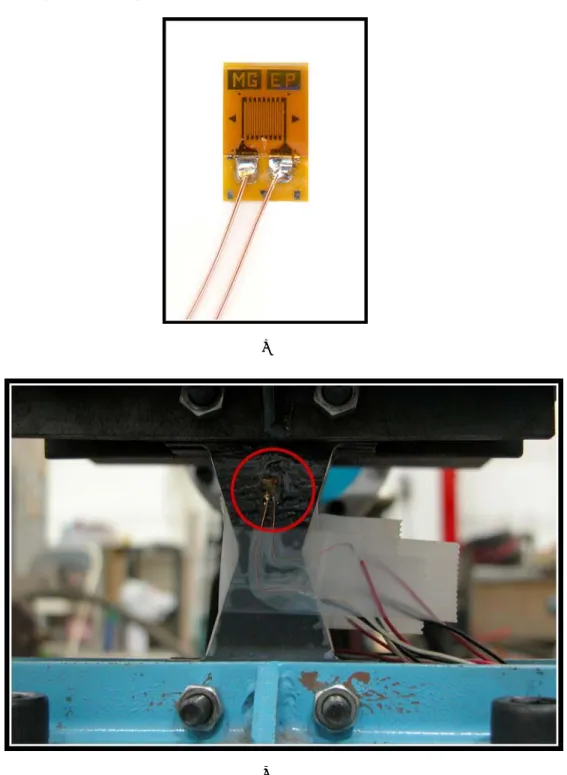
Fig. 3.6 Metallic yielding damper bonded with a piece of strain gauge... 38

Fig. 3.7 The pseudo code for finding the corresponding stresses... 41

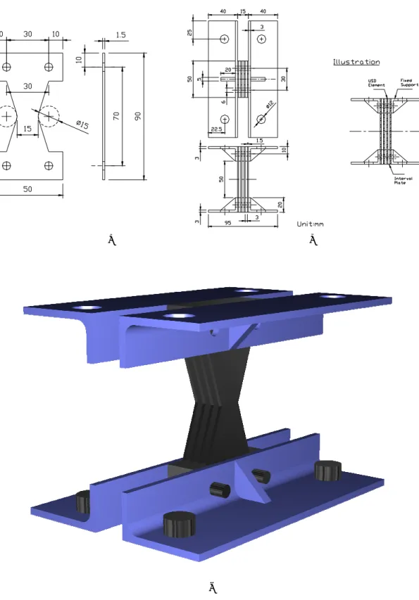
Fig. 4.1 Design of scaled-down metallic yielding damper ... 46

Fig. 4.2 MTS 407 Controller ... 47

Fig. 4.3 1.5-ton actuator of MTS ... 47

Fig. 4.4 Loadcell ... 48

Fig. 4.5 Data acquisition system ... 48

(10)

- viii -

Fig. 4.10 The loading history specified for the component test of scaled-down damper... 53

Fig. 4.11 Hysteresis for directly measured force-displacement relationship of the scaled-down damper ... 56

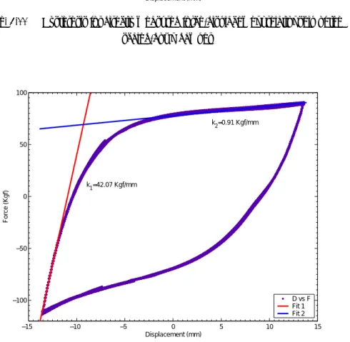
Fig. 4.12 Curve fitting for determining the experimental stiffness of the scaled-down damper ... 56

Fig. 4.13 Measured strain data from component test of scaled-down damper ... 57

Fig. 4.14 Predicted stress-strain hysteresis of the scaled-down damper... 57

Fig. 4.15 Comparison of the hystereses for force-displacement relationship between directly measured and predicted results ... 58

Fig. 4.16 Illustration of the movement of the actuator ... 60

Fig. 4.17 Design of the full-scale metallic yielding damper... 62

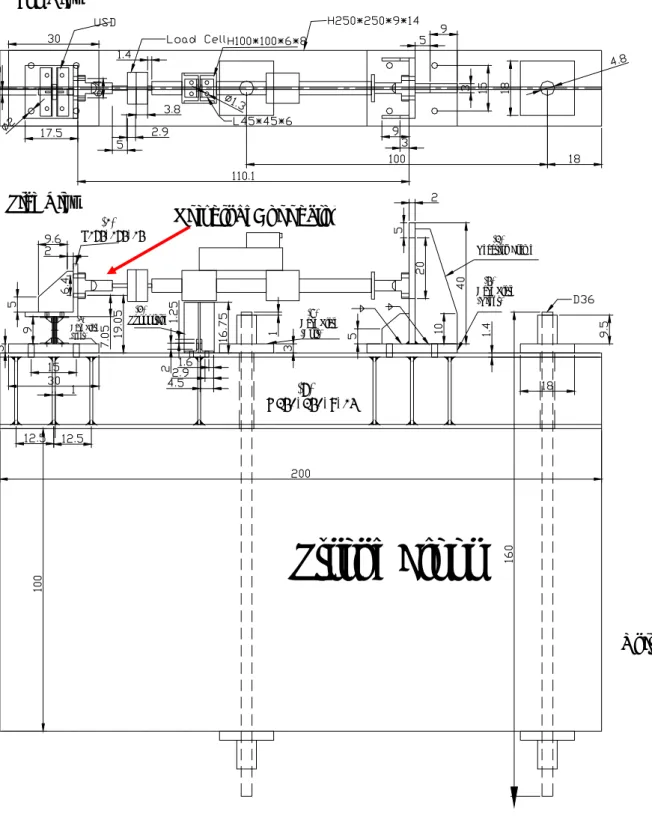
Fig. 4.18 MTS control system in the control room... 63

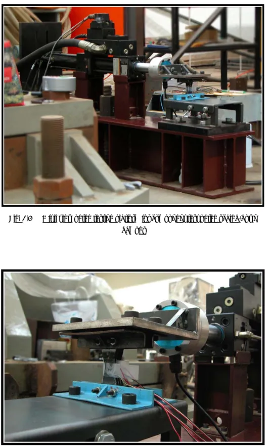
Fig. 4.19 A close-up view of the full-scale damper in testing ... 64

Fig. 4.20 Design sketch of the testing platform for component test of a full-scale damper (Unit: mm)... 65

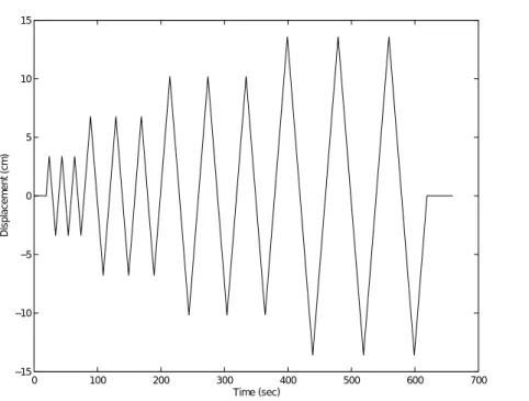
Fig. 4.21 The loading history specified for component test of full-scale damper ... 66

Fig. 4.22 Experimental hysteresis loop of the full-scale damper ... 68

Fig. 4.23 Curve fitting for determining the experimental stiffness of the full-scale damper .. 68

Fig. 5.1 The model structure for shaking table test... 71

Fig. 5.2 Earthquake simulator -- shaking table system ... 74

Fig. 5.3 15-ton dynamic actuator of MTS ... 74

Fig. 5.4 Seismic performance test of the damper on a model structure via shaking table.... 77

Fig. 5.5 A close-up view of a unit of the damper on the model structure... 77

Fig. 5.6 Time history of El Centro earthquake ... 79

Fig. 5.7 Time history of Hachinohe earthquake ... 79

Fig. 5.8 Time history of Kobe earthquake ... 80

Fig. 5.9 Comparison of floor acceleration responses (El Centro, PGA=0.1g) ... 84

Fig. 5.13 Comparison of storydrift of the 1st Floor (El Centro, PGA = 0.1g)... 88

Fig. 5.17 Comparison of Floor Acceleration Responses (Hachinohe, PGA = 0.1g) ... 90

(11)

- ix -

Fig. 5.21 Comparison of Storydrift of the 1st Floor (Hachinohe, PGA = 0.1g) ... 94

Fig. 5.25 Comparison of Floor Acceleration Responses (Kobe, PGA = 0.1g) ... 96

Fig. 5.29 Comparison of Storydrift of the 1st Floor (Kobe, PGA = 0.1g) ... 100

Fig. 5.33 The analytical model of the 5-story model structure (bare frame) established by SAP2000... 114

Fig. 5.34 The analytical model of the 5-story model structure (damper-implemented frame) established by SAP2000 ... 115

Fig. 5.35 The parameters for the frame/cable element specified for the beams and columns in the model structure (Unit: cm) ... 116

Fig. 5.36 The parameters for the frame/cable element specified for the bracing system in the model structure (Unit: cm) ... 116

Fig. 5.37 The parameters for the shell element in the model structure (Unit: cm)... 117

Fig. 5.38 The parameters for the plastic (Wen) element in the model structure (Unit: mm, Kgf) ... 117

Fig. 5.39 The definition of parameters for the Wen’s Plasticity Property... 118

Fig. 5.40 Comparison of acceleration responses of the bare-frame model (Case 1: El Centro, PGA=0.1g)... 121

Fig. 5.41 Comparison of acceleration responses of the bare-frame model (Case 2: Hachinohe, PGA=0.1g)... 122

Fig. 5.42 Comparison of acceleration responses of the bare-frame model (Case 3: Kobe, PGA=0.1g)... 123

Fig. 5.43 Comparison of acceleration responses of the damper-implemented frame model (Case 4: El Centro, PGA=0.1g) ... 124

Fig. 5.44 Comparison of acceleration responses of the damper-implemented frame model (Case 5: El Centro, PGA=0.4g) ... 125

Fig. 5.45 The hystereses of the damper (Case 5: El Centro, PGA=0.4g) ... 126

Fig. 5.46 Comparison of acceleration responses of the damper-implemented frame model (Case 6: Hachinohe, PGA=0.1g) ... 127

Fig. 5.47 Comparison of acceleration responses of the damper-implemented frame model (Case 7: Hachinohe, PGA=0.25g) ... 128

Fig. 5.48 The hystereses of the damper (Case 7: Hachinohe, PGA=0.25g)... 129 Fig. 5.49 Comparison of acceleration responses of the damper-implemented frame model

(12)

- x -

Fig. 5.51 The hystereses of the damper (Case 9: Kobe, PGA=0.25g)... 132 Fig. 5.52 Assessments of seismic performance of the damper (Case 4: El Centro, PGA=0.1g)

... 133 Fig. 5.53 Assessments of seismic performance of the damper (Case 5: El Centro, PGA=0.4g)

... 134 Fig. 5.54 Assessments of seismic performance of the damper (Case 6: Hachinohe, PGA=0.1g)

... 135 Fig. 5.55 Assessments of seismic performance of the damper (Case 7: Hachinohe, PGA=0.25g)... 136 Fig. 5.56 Assessments of seismic performance of the damper (Case 8: Kobe, PGA=0.1g).. 137 Fig. 5.57 Assessments of seismic performance of the damper (Case 9: Kobe, PGA=0.25g) 138

(13)

- xi -

List of Tables

Table 3.1 Parameters and turning points considered for an example of the Ramberg-Osgood

Hysteresis Model ... 35

Table 4.1 Numerical values of parameters for the scaled-down damper ... 45

Table 4.2 Calculated mechanic properties of the scaled-down damper ... 45

Table 4.3 Comparison between the experimental and theoretical stiffness for the scale-down damper ... 54

Table 4.4 Parameters obtained from the component test for the analytical models of the scaled-down damper ... 55

Table 4.5 Numerical values of parameters in the Ramberg-Osgood Hysteresis Model for the methodology of measuring shear force ... 55

Table 4.6 Numerical values of parameters for the full-scale damper ... 61

Table 4.7 Calculated mechanic properties of the full-scale damper... 61

Table 4.8 The reduction factor and stiffness of the full-scale damper ... 67

Table 4.9 Comparison between the experimental and theoretical stiffness for the full-scale damper ... 67

Table 5.1 Detailed properties of the model structure... 72

Table 5.2 Natural Frequency and Damping Ratio of the Model Structure Extracted from System Identification Analysis... 72

Table 5.3 Comparison of Peak Floor Acceleration Responses in the El Centro Series of Tests102 Table 5.4 Comparison of Root-Mean-Squares Floor Acceleration In the El Centro Series of Tests... 103

Table 5.5 Root-Mean-Squares of 1st Floor Storydrift In the El Centro Series of Tests ... 104

Table 5.6 Equivalent Natural Frequency and Damping Ratio of the damper-Protected Model Structure... 104

Table 5.7 Comparison of Peak Floor Acceleration Responses in the Hachinohe Series of Tests ... 105

Table 5.8 Comparison of Root-Mean-Squares Floor Acceleration In the Hachinohe Series of Tests... 106

Table 5.9 Root-Mean-Squares of 1st Floor Storydrift In the Hachinohe Series of Tests ... 107

Table 5.11 Comparison of Peak Floor Acceleration Responses in the Kobe series Tests ... 108

Table 5.12 Comparison of Root-Mean-Squares Floor Acceleration for Kobe Series of Tests109 Table 5.13 Root-Mean-Squares of 1st Floor Storydrift for Kobe Series of Tests... 110

Table 5.15 Analysis cases defined in SAP2000 ... 113

(14)

(15)

(16)

1.1 Background

Before human beings understood the origins of such terrifying natural phenomena as diseases and earthquakes, many thought that these phenomena were God’s punishment for sin. The germ theory of disease, which was proposed in the late 19th_{century, provided a physical explanation for the}

origin of illness. More recently, the genesis of earthquake has also been elucidated in a similar fashion. Most scientists believe that the earth’s shell is made up of twelve large, rigid plates (Fig. 1.1) [1]. These plates move at a rate of only a few centimeters a year, but the effect of this movement, earthquake, is spectacular.

Fig. 1.1 The earth’s seismicity outlines plate margins

There is a saying among geologists and engineers that earthquakes don’t kill but buildings do. Shaking ground may make people fall down, and falls may breaks legs and arms, but they don’t kill. However, shaking ground can make structures collapse, and collapsing structures can definitely kill [1]. Though this is just an old saying, how to prevent the structures from collapse is a serious and complex problem.

(17)

Chapter 1 Introduction 3

The worst earthquake of the twentieth century occurred on July 28, 1976. At 3:45 A.M., while 1 million inhabitants of Tang Shan, China, slept, a 7.8 magnitude quake leveled the city. Hardly a building was left standing; the few that did withstand the first quake were destroyed by the second, magnitude 7.1, which stuck at 6:46 P.M. the same day. Losses were large because most of the buildings had not been constructed to withstand earthquakes [1].

The study of origin of earthquake is the field of earth science, while a branch of civil engineering, Earthquake Engineering, devotes to seeking solutions for protecting people from catastrophes rising from earthquakes. The structural design involving resistance of earthquake is called seismic design. In early years, conventional seismic design practice permits the reduction of design forces below the elastic level on the premise that inelastic action in the structures will provide significant energy dissipation potential which enables them to survive severe earthquakes without collapse [2]. The inelastic action is intended to occur in specially detailed critical regions of the structure, usually in the beams near or adjacent to the beam-column joints. While being able to dissipate earthquake input energy, the inelastic behavior (eg: forming plastic hinge) in these regions also may result in significant damage to the structural members. The structures may survive the earthquake if the inelastic behavior did happen in the way one expected. However, the actual failure pattern of most collapsed or severely damaged structures often was not in that preferable manner, as observed in the 921 Chi-Chi earthquake in Taiwan as well as other major events worldwide. Plastic hinges have never ever been found in the beams due to a substantial increase in rigidity reinforced by the slabs and walls, which in turn minimized the bending curvature of the beams and prevented them from yielding. The actual damage situation contradicts the concepts of traditional seismic design. Without plastic hinges dissipating the earthquake input energy, damages concentrate on the weakest parts of structures, leading to early collapse.

To overcome the inherent shortcomings of the conventional seismic design, a number of innovative approaches have been developed in recent years. Modern seismic structural design, if successfully applied, not only can save people’s lives but also minimize the impacts on economy and society in

(18)

severe earthquake. The main idea of modern seismic design is that performances of a structure under different intensity of earthquake are accounted for. To achieve desirable seismic performance, the traditional method of increasing the dimension of structural members for earthquake-resistance is discarded by introducing energy dissipation systems, control systems or seismic isolation systems into the structural design. These systems will be briefly introduced in the next section.

(19)

1.2 Structural Protective Systems

By considering the dynamic nature of environmental disturbances, more dramatic improvements in seismic structural design can be realized. New and innovative concepts on structural protection have been advanced and at various stages of development in recent years. Modern structural protective systems can be divided into 3 major groups [3]:

1. Passive Energy Dissipation 2. Seismic Isolation

3. Active / Semi-Active Control

Each group consists of several technologies as shown in Fig. 1.2. These strategies for seismic protection of structures will be introduced briefly.

Structural Protective Systems Structural Protective Systems 1. Passive Energy Dissipation 2. Seismic Isolation 3. Active / Semi-active Control

1. Metallic Yielding Dampers 2. Friction Dampers 3. Viscoelastic Dampers 4. Viscous Fluid Dampers 5. Tuned Mass Dampers 6. Tuned Liquid Dampers 1. Elastomeric Systems 2. Sliding Systems 3. Rocking systems Structural Protective Systems Structural Protective Systems 1. Passive Energy Dissipation 2. Seismic Isolation 3. Active / Semi-active Control

1. Metallic Yielding Dampers 2. Friction Dampers 3. Viscoelastic Dampers 4. Viscous Fluid Dampers 5. Tuned Mass Dampers 6. Tuned Liquid Dampers 1. Elastomeric Systems 2. Sliding Systems 3. Rocking systems

(20)

1.2.1 Passive Energy Dissipation

A passive energy dissipation system does not require an external power source. Passive energy dissipation devices impart forces that are developed in response to the motion of the structure. The energy in a passively controlled structural system, including the passive devices, cannot be increased by the passive control devices. [4] The basic energy relationship of the structures is represented in the following equation [5]:

I K S H

E

=

E

+

E

+

E

_ξ

+

E

(1.1)

where

I

E

= earthquake input energy

K

E

= kinetic energy in structure

S

E

= strain energy in structure

E

ξ = viscous damping energy

H

E

= hysteretic damping energy

The aim of including energy absorbers in a structure for earthquake resistance is to concentrate hysteresis behavior in specially designed and detailed regions of the structure and to avoid inelastic behavior in primary gravity-load resisting structural members. In other words, the goal is to increase

E

_H so that, for a given

E

_I , the elastic strain energy in the structure is minimized. This means that the passively controlled structure will undergo smaller deformations for a given level of input energy than the one without energy dissipators. The major energy dissipation devices available are as follow [4]:

1. Metallic Yielding Dampers 2. Friction Dampers

3. Viscoelastic Dampers 4. Viscous Fluid Dampers 5. Tuned Mass Dampers 6. Tuned Liquid Dampers

(21)

Metallic Yielding Dampers One of the effective mechanisms available for seismic energy dissipation is through inelastic deformation of metals. The idea of utilizing added metallic energy dissipators within a structure to absorb a large portion of seismic energy began with the conceptual and experimental work of Kelly et al. (1972) and Skinner et al. (1975). The devices considered included torsional beams, flexural beams, and U-strip energy dissipators (Fig. 1.3). In recent years, a wide variety of such devices have been proposed. Many of these devices use mild steel plates with triangular or hourglass shapes so that yielding is spread almost uniformly throughout the material. A typical X-shaped added damping and stiffness (ADAS) device (Bergman and Goel, 1987 and Whittaker et al. 1991), triangular ADAS (TADAS) (Tsai et al. 1993) and reinforced ADAS (RADAS) (Tsai, 1999) are shown in Fig. 1.4, Fig. 1.5 and Fig. 1.6, respectively.

Fig. 1.3 Several metallic yielding devices (a) Torsional Beam (b) Flexure Beam (c) U-strip

(22)

(a) (b) (c) Fig. 1.4 ADAS

(a) A photo of ADAS Unit (Bergman and Goel, 1987)

(b) Front view of ADAS element (Whittaker et al. 1991) (c) Side view of ADAS unit

Fig. 1.5 A photo and detailed design of TADAS

Fig. 1.6 A photo of RADAS1

(23)

Despite apparent differences in geometric configuration, the underlying energy dissipative mechanism for the above mentioned devices results from inelastic deformation of the metallic elements. Therefore, one must be able to characterize their hysteretic behavior under arbitrary cyclic loading. Ideally, one would hope to develop a model of any metallic device starting from micromechanical theory of dislocations [6]. However, since a direct physics approach is not yet feasible, one normally accepts a macroscopic level of description. Özdemir (1976) was the first to consider the modeling problem of material inelasticity. Shortly later, Bhatti et al. (1978) employed Özdemir’s methodology to study the response of structures that used torsional bar dampers along with a seismic base isolation system. Dargush and Soong (1995) developed an inelastic constitutive model for the material of metallic yielding dampers based on a microscopic mechanistic approach and compared it with experimental data for validation. Tsai (1995) developed a finite-element formulation for ADAS and compared the simulation results with experimental data.

The hysteretical behavior of the metallic damper can be obtained via component tests of the device [4]. In case only the strains are measured, a basic form of the nonlinear stress-strain relationship is first selected, and then the related model parameters are determined via curve fitting or a macroscopic mechanical analysis of the device. By this approach, any admissible hysteretic model, such as the bilinear model, may be selected. Ou and Wu (1995) explored the hysteretical behavior of both X-shaped and triangular metallic dampers by employing a bilinear model with parameters related to size and material properties. The ultimate displacements of the devices were also determined.

The earliest applications of metallic yielding dampers to structural systems appeared in South Rangitikei viaduct in New Zealand2_{. The dampers}

were installed in the pier base to control the rocking action of the bridge. Recently, ADAS devices have been installed in buildings in Italy, USA, Mexico, Japan and Taiwan for earthquake protection.

(24)

Friction Dampers Friction provides another means of energy dissipation which has been utilized for years in automotive brakes to dissipate kinetic energy of motion. In structural engineering, a wide variety of devices differing in mechanical complexity and materials have been proposed and studied. Most friction damper utilizes interfaces of steel on steel, brass on steel, or graphite impregnated bronze on stainless steel. Composition of the interface is of great importance to insure longevity of the devices. A friction device developed by Pall (1982) is shown in Fig. 1.7 [4].

Fig. 1.7 Pall Friction Device

Viscoelastic Dampers The metallic and frictional devices are primarily intended for seismic application. Some viscoelastic solid materials, on the other hand, are used for dissipating energy at all deformation levels that allows them for both wind and seismic protection [4].

The application of viscoelastic materials to vibration control dates back to the 1950s for aircrafts as a means of controlling the vibration-induced fatigue in airframes. Their application to civil engineering structures appear in 1969 for the former World Trade Center in New York where approximately 10,000 viscoelastic dampers were installed in each of the twin towers to reduce wind-induced vibrations.

A typical viscoelastic damper, developed by the 3M Company Inc., is shown in Fig. 1.8. It consists of viscoelastic layers bonded in between steel plates. It is worthwhile pointing out that the viscoelastic material is linear over

(25)

a wide range of strain provided that the temperature is constant. At large strains, there is a considerable self-heating due to a large amount of energy dissipated. The generated heat changes the mechanical properties of the material, and the overall behavior becomes nonlinear and deteriorated.

Fig. 1.8 A viscoelastic damper

Viscous Fluid Dampers Fluids can also be used for energy dissipation. Numerous configurations and materials have been considered for such type of devices. One class involves the use of a cylindrical piston immersed with viscoelastic fluid. Such systems have been studied both experimentally and analytically by Makris et al. (1993). Another device referred to as the viscous damping wall, again use viscoelastic fluid (Arima et al. 1988; Miyazaki and Mitsuaka 1992) [4].

Viscous fluid dampers widely used in aerospace and military applications recently have found applications in structural engineering (Constantinou et al. 1993). Characteristics of these devices that are of primary interest in structural applications are the linear viscous response achieved over a broad frequency range, insensitivity to temperature and compactness in terms of small stroke requirement with considerable output force.

It should be pointed out that most, if not all, viscous fluid dampers currently in use have a force-velocity relationship of the form

sgn( )

F C V

=

α

V

where

F

is the damping force,

C

is dependent on ambient temperature,

V

is the relative velocity in between the damper, and

α

is an exponent in the range

0.3 ≤ ≤

α

0.75

. Major advantages of this type of nonlinear dampers are that the force builds up fast at small velocity

(26)

and tends to flatten out at higher velocities. A typical fluid damper is shown in Fig. 1.93_.

Fig. 1.9 A Fluid Damper

Tuned Mass Dampers Tuned mass damper (TMD), first proposed by Frahm [7], as a secondary system to control the primary structure generally consists of a mass block with damping and tuning elements. The frequency of a TMD system is tuned by adjusting the stiffness of the spring (sliding type) or the arm length of the suspension cable (pendulum type) [8] to be in near-resonance with the primary structure. As a result, a considerable vibrating energy can be transferred from the primary structure to the TMD system and then dissipated via the damping mechanism of its own. In general, the TMD system is effective in the control of wind-induced structural vibrations. Many well-known skyscrapers, such as the Citibank in New York, the John Hancock Tower in Boston4_{, the CN Tower in Toronto}5_{, and Taipei 101}

in Taipei (Fig. 1.10) adopt TMD for wind-resistance.

Fig. 1.10 Buildings installed with TMD (a) John Hancock Tower in Boston (b) CN Tower

(c) TMD in Taipei 101 (d) Taipei 101

3_{http://www.e-structures.com/viscous.html} 4 _{http://www.bluffton.edu/HomePages/FacStaff/sullivanm/peihancock/peihancock.html} 5 _{From a postcard} (d) (c) (b) (a)

(27)

Tuned Liquid Dampers Conceptually similar to a TMD system, Tuned Liquid Damper (TLD) has been increasingly used in high-rise buildings for wind or earthquake induced vibration control [9,10]. The TLD can be integrated with the existing fire-suppress hydraulic tower and therefore considered a substitution of the TMD for economic reasons. The TLD can be further classified into the Tuned Sloshing Water Damper (TSWD) and the Tuned Liquid Column Damper (TLCD)[11-17]. The frequency of the TSWD is adjusted by changing the depth of the storage water as well as the geometry of the tank. Damping of the TSWD is produced via steel wire nets across the water passage, through which turbulent flow is generated and energy dissipated. While the frequency of the TLCD depends only on the total length of the water in the U-shape container, and damping of the TLCD due to headloss of the water is introduced by changing the dimension of the orifice (valve) or adjusting the cross sectional area of the U-shape container. For TSWD, only the sloshing motion of the near-surface portion of the water contributes in the control, while for TLCD, all the water is effective.

1.2.2 Seismic Isolation

Seismic isolation systems may be further classified into 3 categories: [18] 1. Elastomeric Systems

2. Sliding Systems 3. Rocking systems

Elastomeric Systems With lateral flexibility and vertical rigidity, elastomeric bearings may shift (lengthen) the natural period of the structure away from the predominant period of the ground motion (stiff soil conditions) to reduce earthquake forces. By introducing either the damping-enhanced rubber or supplemental energy dissipative components, the seismic isolation system may avoid excessive bearing displacement during severe earthquakes. The elastomeric bearings that have seen widespread applications include the lead-rubber bearing (LRB) and high-damping rubber bearing (HDRB) [19-21].

(28)

Sliding Systems Sliding systems reduce seismic forces via the friction mechanism between the sliding interfaces. The sliding-type bearings in its original form, however, are impractical due to lack of restoring capability. To overcome this problem, the friction pendulum system (FPS) introduces a spherical sliding interface to provide restoring stiffness with the friction mechanism playing the role of energy dissipation. As a result, FPS is functionally equivalent to LRB and HDRB in altering the structure’s fundamental period. Made of stainless steel, the properties of FPS are less sensitive to aging and temperature. The bearing’s high strength and rigidity make them compact in size, which may further reduce the installation cost. With versatile features of period-invariance, torsion-resistance, temperature-insensitivity and durability, FPS meets the diverse requirements of seismic isolation for buildings, bridges and industrial facilities [22-32].

Rocking Systems Rocking mechanism is another means of seismic isolation, although it is rarely conceived this way. With a discontinuous interface between the columns and the underlying foundation, the rocking system is allowed to rock intermittently as the seismic overturning moment exceeds the restoring moment contributed by gravity. The boundary condition at the footing changes from being “fixed” to “hinging” as soon as the uplift occurs, accompanied with a sudden release from the moment-resisting status as a consequence. The earthquake load is then counteracted by the rotational inertia of the structure with respect to the supporting foot. In other words, the rocking mechanism provides a unique means to filter out earthquake energy. Rocking system is particularly effective in reducing the seismic loads and deformations of structures with heavy superstructure such as water tanks supported by tower or bridges with tall and slender pier (Priestley et al. 1996). The concept of rocking mechanism has been adopted for a railway bridge (Beck and Skinner 1974) and industrial chimney in New Zealand (Sharpe and Skinner 1983). Recently, utilization of rocking mechanism for earthquake protection of bridge structures has become a renewed interest (Mander and Cheng 1997, Wang et al. 2001).

(29)

1.2.3 Active / Semi-Active Control System

An active control system is one in which an external source powers control actuator(s) that apply forces to the structure in a prescribed manner. These forces can be used to both add and dissipate energy in the structure. In an active feedback control system, the signals sent to the control actuators are functions of the response of the system measured with vibration sensors [4].

Semi-active control systems are a class of active control system for which the external energy requirements are smaller than those for typical active control systems. Typically, semi-active control system devices do not add mechanical energy to the structural system (including the structures and the controlling actuators), therefore bounded-input bound-output stability is guaranteed. Semi-active control devices are often viewed as controllable passive devices.

The most challenging aspect of active control research in civil engineering is the fact that it is an integration of a number of diverse disciplines, some of which are beyond the domain of traditional civil engineering. These include computer science, data processing, control theory, material science, as well as stochastic processes, dynamic structural theory, and wind and earthquake engineering.

(30)

1.3 The Organization

Chapter 1 The modern structural protective systems including energy dissipation systems, control systems and seismic isolation systems have been introduced briefly.

Chapter 2 The fundamentals of the metallic yielding damper including determination of stiffness, yielding displacement, yielding load and design considerations have been introduced in this chapter.

Chapter 3 A novel methodology for measuring the moment and shear force of the metallic yielding damper based on strain measurement and Ramberg-Osgood Hysteresis Model is developed. A table searching method is proposed to overcome numerical difficulties due to the high nonlinearity of equations in this model.

Chapter 4 Component tests for both full-scale and scaled-down dampers have been tested independently. The first objective of the component tests is to investigate the characteristics of individual unit under cyclic loadings. The second one is to verify the measuring methodology for moment and shear via strain measurement. The final one is to determine the parameters of the damper for the analytical models characterizing the inelastic behavior to be used by SAP2000.

Chapter 5 In order to assess the effectiveness and feasibility of the damper through the earthquake, a series of shaking table test have been conducted. The analytical SAP2000 models are established to simulate the responses of structures under various earthquakes scenarios. The simulating results are compared with the experimental ones.

Chapter 6 Based on the testing results, the conclusions are drawn in this chapter.

(31)

Fundamentals of

Metallic Yielding Damper

(32)

2.1 Introduction

Metallic yielding damper is an earthquake protective device that dissipates earthquake energy through inelastic deformation of steel plates. Each of its plates is tailored into an optimum shape (X-shape) to maximize its energy dissipative capacity. The damper can be designed to yield at moderate deformation so as to protect the structure at early stages. If the dampers are tactfully sized and allocated, both the acceleration and displacement responses of the structure can be simultaneously reduced during severe earthquake.

In this chapter, fundamentals of the X-shaped metallic yielding damper will be introduced. These include the determination of stiffness, yielding displacement, yielding loads and design considerations. This chapter is concluded with a parametric analysis of the damper.

(33)

Chapter 2 Fundamentals of Metallic Yielding Damper 19

2.2 Theoretical Derivations

(a) (b) (c) Fig. 2.1 X-shaped metallic yielding damper

(a) 3-D view of a single plate of the metallic yielding damper (b) Front view (c) Side view of the deformed plate

A 3-D view of a single plate of the metallic yielding damper is shown in Fig. 2.1(a) where

B

,

h

,

t

and

b

are the end width, effective height, thickness and the narrowest width (neck) of the plate, respectively. Defining the x-coordinate as in Fig. 2.1(b), one can express the cross-sectional width at any arbitrary distance

x

from its upper end for the upper half of the plate as

2 ( )

(

) , 0

2 h

b x

B

b B x

x

h

=

+

−

≤ ≤

(2.1)

The corresponding cross-sectional area and moment of inertia about the neutral axis of the area are, respectively,

2 ( )

( )

(

)

, 0

2 h

A x

b x t

B

b B x t

x

h

⎡

⎤

⎢

⎥

=

+

−

≤ ≤

⎢

⎥

⎣

⎦

(2.2) 3 3

1

2 ( )

( )

(

)

, 0

12

2 h

I x

b x t

B

b B x t

x

h

⎡

⎤

⎢

⎥

=

+

−

≤ ≤

⎢

⎥

⎣

⎦

(2.3)

(34)

The moment on the cross-section at a distance

x

from the upper end can be obtained from equilibrium as

(

)

2 ( )

2

1

2

2 P

Ph

x

M x

h

x

h

⎛

_⎞⎟

⎜

=

−

=

_⎜

_⎜⎝

−

⎟

_⎟

⎠

(2.4)

where

P

is the lateral force acting on the upper end.

The curvature of the plate in bending can be expressed, in accordance with mechanics of materials, as

[

]

3

( )

6 (

2 )

( )

2(

)

M x

Ph h

x

EI x

E Bh

b B x t

κ

=

−

+

−

(2.5)

where

E

is the Young’s Modulus of the material and

κ

denotes the curvature. This equation shows that the curvature is directly proportional to the bending moment and inversely proportional to flexural rigidity,

EI

, which is a measure of the member’s resistance to bending.

Idealized X-shaped Damper First we consider the idealized X-shaped plate whose neck width reduces to 0, assuming

E

to be constant, then Eq. (2.5) can be reduced to 3 0

6 lim ( )

.

b

Ph

x

const

EBt

κ

→

=

(2.6)

This equation shows that the curvature of each cross-section all over the damper is identical, meaning that the yielding initializes and develops simultaneously at all cross-sections.

Taking both the flexural and shear strain deformation into account, one can express the total strain energy in the plate as it deforms (Fig. 2.1(c)) to be

[

]

2

[

]

2 2 2 0 0

( )

1

2

2 ( )

2

2 ( )

h h

M x

V x

U

dx

EI x

β

GA x

⎛

_⎞⎟

⎜

_⎟

⎜

_⎟

⎜

=

_⎜

+

⎟

_⎟

⎜

_⎟⎟

⎜

⎟

⎜⎝

∫

⎠

(2.7)

in which

β

is the shape factor taken as 5

(35)

As the damper is subjected to the lateral force

P

(Fig. 2.1(b)), the deformation due to this force can be found by using Castigliano’s Theorem as follow: [ ] [ ] 2 2 0 0 ( ) ( ) ( ) ( ) ( ) 2 ( ) 2 h h M x V x M x V x P _dx P _dx EI x G A x U P _β ∂ ∂ ∂ ∂ ∆ = ∂ = ₊ ∂

⎛

_⎡

_⎤

_⎡

_⎤

_⎞⎟

⎜

_⎟

⎜

_⎢

_⎥

_⎢

_⎥

_⎟

⎜

_⎟

⎜

⎣

⎦

⎣

⎦ ⎟

⎜

_⎟⎟

⎜

_⎟

⎜

_⎟

⎜

_⎟

⎜⎝

∫

⎠

(2.8)

Carrying out the integration, one gets

[

]

3 2 2 2 2 3 3 3 4 3 2 ln( ) 2 ln( ) (ln ln ) 2 ( ) 2 ( ) h Bb b B b bh b Bh h b B P Et b B βGt b B − − + − − ∆ = + − −

⎧

⎫

⎪

⎨

⎬

⎪

⎩

⎭

(2.9)

Consequently, the elastic stiffness of the damper is given by

[

]

3 2 2 2 2 3 3 1 3 4 3 2 ln( ) 2 ln( ) (ln ln ) 2 ( ) 2 ( ) d P k h Bb b B b bh b Bh h b B Et b B βGt b B = = − − + − ∆ − + − − (2.10) 0 5 10 15 20 25 30 1.5 2 2.5 3 3.5 4 4.5

The neck width (b) of the damper (cm)

Difference (%)

Fig. 2.2 Error of neglecting shear deformation on stiffness

d d d

k

−

(%)

(36)

If we neglect the effects of shear deformation, the right term of the dominator in Eq. (2.10) vanishes. Thus, the elastic stiffness can then be written as

3 3 3 2 2 2 2

2 (

)

3

4

3 2 ln(

) 2 ln(

)

d

Et b B

k

h

Bb

b

B

b

bh

b

Bh

−

=

_⎡

_⎤

−

+

−

⎢

⎥

⎣

⎦

(2.11)

For a given neck width of the damper, difference between the stiffness calculated by using the exact stiffness (Eq. (2.10)) and the simplified one (Eq. (2.11)) ranges from 1.5%~4.5%, as shown in Fig. 2.2. In other words, the effect of shear deformation on overall stiffness is insignificant and can therefore be neglected.

By further considering the neck width to be zero, for simplicity, the elastic stiffness for one single plate of the X-shaped metallic yielding damper can be simplified as 3 3

2

3

d

EBt

k

h

′ =

(2.12)

The elastic stiffness for a unit consisting of

N

identical plates in parallel can be calculated as follows: 3 3

2

3

d

NEBt

k

h

′ =

(2.13)

The yielding moment in the upper or lower end is

2 0 2

6

y x y y _t

I

Bt

M

₌

σ

=

₌

σ

(2.14) where

σ

_y is the yielding stress of the material of the plate. The yielding load,

y

P

, can then be found by dividing the yielding moment by half of the height of the damper. That is,

2 2

3

y y y _h

M

Bt

P

h

σ

=

(2.15)

The plastic moment,

M

_p, at the upper or lower end is 1.5 times that of the yielding moment for rectangular X-sections, and plastic load,

P

_p, can in turn be calculated as 2 2 2

1.5

2

p y y p _h _h

M

Bt

P

h

σ

=

(2.16)

(37)

Finally, the idealized yielding displacement can be calculated by the following equation: 2

2

y y y d

P

h

k

Et

σ

′

∆ =

=

′

(2.17)

2.3 Design Considerations

To avoid undesired shear failure of the damper at the neck prior to full development of the ultimate flexural strength, a minimum width of the neck is required. If the ultimate lateral force is considered as 1.5 times the plastic load, the following inequity should be met to ensure that the shear strength of the damper is sufficient, i.e.,

1.5

s u p

S

≥

P

=

P

(2.18)

where

P

_u and

S

_s are the ultimate load and shear strength of the damper, respectively. The shear strength equals to the cross-sectional area multiplied by the allowable stress, taken as 0.55 times the yielding stress, that is,

0.55

s y

S

=

σ

bt

(2.19)

Combining Eq. (2.16), (2.18) and (2.19), the minimum neck width of the damper can be determined as follows:

1.36 Bt

b

h

(38)

2.4 Parametric Analysis

It is observed from the analysis in the previous section that the elastic stiffness and yielding displacement of the metallic yielding damper depend on height-to-thickness ratio

(

h t

)

of the damper. The differences between the exact stiffness, Eq. (2.11), and the idealized one, Eq. (2.13), can be revealed by performing parametric analyses.

The stiffness ratio

(

k k′d d

)

with respect to the height-to-thickness ratio is

plotted in Fig. 2.3 for various safety factor

(

SF

)

defined as

1.36 b t

SF

t h

=

(2.21)

The difference between the exact stiffness and idealized one decreases with height-to-thickness ratio increased.

The idealized formula underestimates the stiffness of the damper as the neck width of the damper becomes large (i.e. higher safety factor in design). Generally speaking, it is recommended to adopt a height-to-thickness ratio of 10 ~ 15 in practical design so that the stiffness ratio

(

k k′_d _d

)

will range from 1.2 to 1.5 while the safety factor is taken as 2 to 4.

SF

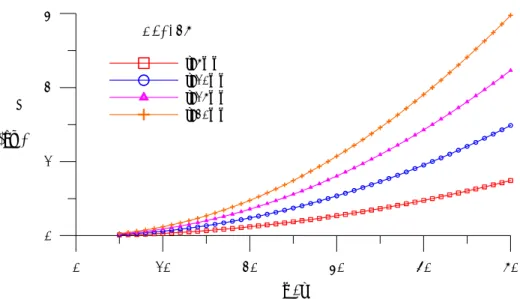
taken as 6, the relation between the stiffness ratio and the height-to-thickness ratio is shown in Fig. 2.4. The results show that the difference between exact stiffness and the idealized one is insignificant while the height-to-thickness ration of the damper is lager than 10, which meets the suggested value to be adopted in practical design.

(39)

Chapter 2 Fundamentals of Metallic Yielding Damper 25 0 10 20 30 40 50 h / t 0 1 2 3 K / k eq B=15cm S.F.=2 S.F.=4 S.F.=6 S.F.=8 S.F.=10

(

k k′ with respect to height-to-thickness ratio _d _d

)

(

h t for

)

various safety factors

( )

SF

0 10 20 30 40 50 h / t 0 0.5 1 1.5 2 2.5 K / k eq B=15cm t=5mm t=10mm t=15mm t=20mm

(

k k′ with respect to height-to-thickness ratio _d _d

)

(

h t for

)

various thicknesses

( )

t d d

k

k′

d d

k

k′

6 SF =

(40)

The relationship between the yielding displacement and height-to-thickness ratio is plotted in Fig. 2.5. The results show that the yielding displacement increases as height-to-thickness ratio becomes large under a given thickness of the damper. In addition, yielding displacement depends on the height-to-thickness ratio and the height, meaning that yielding displacement is larger as the height of the damper increases for a given height-to-thickness ratio.

The exact yielding displacement is defined as

y y d

P

k

∆ =

(2.22)

The relationship between the yielding displacement ratio

(

∆ ∆y ′y

)

and

height-to-thickness

(

h t ratio is shown in Fig. 2.6. It is observed that

)

yielding displacement is independent of the thickness of the damper when the height-to-thickness ratio is greater than 15.

(41)

Chapter 2 Fundamentals of Metallic Yielding Damper 27 0 10 20 30 40 50 h / t 0 1 2 3

0

y (c m ) B=15cm t=5mm t=10mm t=15mm t=20mm

Fig. 2.5 Yielding displacement with respect to height-to-thickness ratio

(

h t for

)

various thicknesses of the damper

0 10 20 30 40 50 h / t 0 0.2 0.4 0.6 0.8 1 0 y / 0 yeq B=15cm t=5mm t=10mm t=15mm t=20mm

Fig. 2.6 Height-thickness ratio

(

h t with respect to yielding displacement ratio

)

(

∆ ∆y ′y

)

for various thicknesses of the damper y y

∆

′

∆

B=15cm t=5mm t=10mm t=15mm t=20mm y

∆

(cm)

(42)

(43)

Development of Measuring

Methodology for Moment and

Shear via Strain Measurement

(44)

ε σ ε σ ε σ

To explore the behavior of metallic energy dissipators, characterization of the inelastic stress-strain (or load-displacement) relationship of metals under cyclic loading is demanded. Several mathematical models have been introduced to describe the stress-strain relationship among which the bilinear strain hardening model, the elastoplastic model and the Ramberg-Osgood model shown in Fig. 3.1 are most commonly adopted [33]. In this study, the Ramberg-Osgood Hysteresis Model is employed to describe the stress-strain relationship of the metallic yielding damper.

Fig. 3.1 Common mathematical models for stress-strain relationship

In deriving the hysteresis of a metallic yielding damper in component tests, usually the reacting force of the actuator is measured with a build-in loadcell from a displacement-controlled cyclic loading test. However, it is impractical to implement loadcells, regardless of axial or shear types, for monitoring the actual performance of the damper on site.

In this chapter, a methodology for estimating the moment and shear force of the metallic yielding damper based on strain measurement and Ramberg-Osgood Hysteresis Model is developed. A complete procedure for proposed methodology will be presented.

(45)

Chapter 3 Development of Measuring Methodology for Moment and Shear via Strain Measurement

31

3.1 Ramberg-Osgood Hysteresis Model

3.1.1 Single-loop Model

The stress-strain relationship for several metals, including steel, aluminum and magnesium, can be accurately represented by Ramberg-Osgood equation:

0 0 0 n

σ

ε

σ

_α

σ

ε

=

σ

+

⎛ ⎞⎟

⎜

⎜ ⎟

⎝ ⎠

⎟

(3.1)

where

ε

and

σ

are the strain and stress, respectively, and

α

,

n

,

σ

₀ and

0

ε

are constants to be determined from tension test of the material of the device.

σ

₀ is the proportional (elastic) limit of the material and

ε

₀ is the strain corresponding to

σ

₀ [33].

However, Eq. (3.1) alone is not sufficient for describing the inelastic behavior in cyclic or arbitrary loading conditions where loading and unloading processes occur alternately. A more complete model that traces the unloading and reloading paths of the inelastic behavior has been proposed by Ing and Dorka [34] as

0 0 0

2

n A A A

ε

σ

_α

σ

ε

σ

⎛

⎞

−

₌

−

_⎜

_{− ⎟}

_⎟

+ ⎜

_⎜

_⎟

⎜⎝

⎠

(3.2) and 0 0 0

2

n B B B

ε ε

σ σ

_α

σ σ

ε

σ

⎛

⎞

−

₌

−

_⎜

−

_⎟

+ ⎜

_⎜

_⎟

⎜⎝

⎠

(3.3)

where

ε

A and

ε

B are strains of point A and B, respectively, while

σ

A and B

σ

are stresses at the turning point A and B, respectively (see Fig. 3.2 for a typical single-loop Ramberg-Osgood Hysteresis Model). These two equations combined with Eq. (3.1) for the initial path of the loading constitute a complete hysteresis model. The first equation (the blue line) defines the initial curve starting from the origin. The second (the red line) and third equations (the green line) define the unloading and reloading curves, respectively. These curves actually form a “loop” of the hysteresis.

(46)

0 0 Initial Path Unloading Path Reloading Path ε σ

Fig. 3.2 Typical single-loop Ramberg-Osgood Hysteresis Model

Turning points of the hysteresis are points at which the consecutive governing equations intersect. They are the starting point for generating the Ramberg-Osgood Tables for the path. The strain and stress at turning points are always the local extreme values in the corresponding path.

One may encounter numerical difficulties in determining the stress for a given strain by one of Eq. (3.1)~(3.3) due to high nonlinearity of these equations. Numerical methods such as the Newton-Raphson method and the Secant Method commonly adopted fail to solve the equations for convergence problems due to significant difference in order between the stress and strain [35]. In order to overcome numerical difficulties, a table searching method is proposed in this study.

A

B

A

σ

B

ε

A 0

ε

0

σ

B

σ

(47)

33

To facilitate programming by the proposed table searching method, an alternative form of the model is first derived as

0 0 n

E

σ

σ α

σ

ε

σ

⎛ ⎞⎟

⎜

=

+

_{⎜ ⎟}

⎟

⎝ ⎠

(3.4) 0 0

2

n A A A

E

σ α

σ

ε

σ

⎛

⎞

−

_⎜

_{− ⎟}

_⎟

=

−

⎜

_⎜

_⎟

⎜⎝

⎠

(3.5) 0 0

2

n B B B

E

σ α

σ σ

ε

σ

⎛

⎞

−

_⎜

−

_⎟

=

+

⎜

_⎜

_⎟

⎜⎝

⎠

(3.6)

in which

E

=

σ ε

₀ ₀ is the modulus of elasticity in the initial portion of the stress-strain curve. Therefore, the strain can be obtained directly for a given stress from one of Eq. (3.4) ~ Eq. (3.6) provided that all the parameters are given and the turning points are identified. Once the turning points are specified, the Ramberg-Osgood Table for the unloading and reloading path can be generated according to Eq. (3.5) and Eq. (3.6), respectively. Note that the initial path needs no turning point for generating the table.

The inelastic relationship between strain and stress is path-dependent and not a one-to-one mapping as governed by Eq. (3.4) ~ Eq. (3.6). One can determine the corresponding stress of a given strain by searching the table only when a certain path is specified.

It has become an industrial practice to use the stress corresponding to 0.002 as the equivalent yielding stress. The stress-strain relationship takes the form [36] 0

0.002

n

E

σ

ε

σ

⎛

_⎞⎟

⎜

_⎟

=

+

⎜

_⎜

_⎟

⎜⎝ ⎠

(3.7)

Comparing Eq. (3.7) with Eq. (3.4), one can write

0

0.002 E

α

σ

=

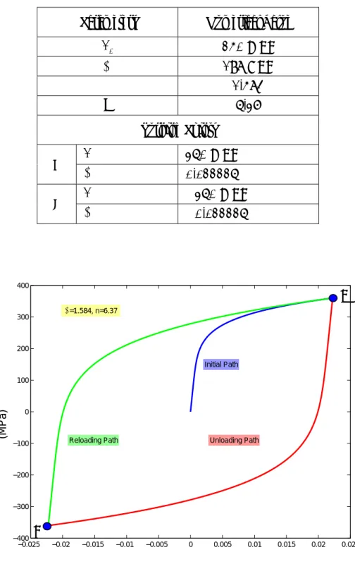
(3.8)

As an illustration, a single-loop Ramberg-Osgood Hysteresis Model is plotted in Fig. 3.3 by assigning numerical values to the parameters and specifying turning points in the equations (Table 3.1). These parameters are

(48)

supposed to be obtained from tension tests for the materials and are suggested by Rasmussen [36]. Note that the turning points depend on the loading path, not necessarily any specific values or symmetric.

(49)

35

Table 3.1 Parameters and turning points considered for an example of the Ramberg-Osgood Hysteresis Model

Parameters Numerical

Value

0

σ

250 MPa

E

198 GPa

α

1.584 n

6.37 Turning Points

A

σ

360 MPa

A A

ε

0.022226

B

σ

−

360 MPa

B B

ε

−

0.022226

−0.025 −0.02 −0.015 −0.01 −0.005 0 0.005 0.01 0.015 0.02 0.025 −400 −300 −200 −100 0 100 200 300 400 α=1.584, n=6.37 Initial Path Unloading Path Reloading Path ε σ (MPa)

Fig. 3.3 Illustration of a single-loop Ramberg-Osgood Hysteresis Model

A

金屬消能制震板之理論分析與實驗

國立交通大學

土木工程學系碩士班

碩 士 論 文