基於人智運算輔助定位分群之群組通訊在耐延遲網路的研究

行政院國家科學委員會專題研究計畫 成果報告

基於人智運算輔助定位分群之群組通訊在耐延遲網路的研

究

研究成果報告(精簡版)

計 畫 類 別 ： 個別型

計 畫 編 號 ： NSC 99-2221-E-004-005-

執 行 期 間 ： 99 年 08 月 01 日至 100 年 09 月 30 日

執 行 單 位 ： 國立政治大學資訊科學系

計 畫 主 持 人 ： 蔡子傑

計畫參與人員： 碩士班研究生-兼任助理人員：陳英明

碩士班研究生-兼任助理人員：林昶瑞

博士班研究生-兼任助理人員：羅文卿

報 告 附 件 ： 出席國際會議研究心得報告及發表論文

公 開 資 訊 ： 本計畫可公開查詢

中 華 民 國 100 年 12 月 29 日

中 文 摘 要 ： 近年來無線網路與 3G 網路的興貣，以及智慧型手機漸漸在

手機市場中嶄露頭角，利用 GPS(Global Position System)

系統搭配地圖程式功能來規劃旅遊路線、玩遊戲、聽音樂

等，現在在智慧型手機上就可以完成。

然而，因為成本的考量與實際上的限制，未必所有的地點都

適合架設無線的 AP，這些沒涵蓋到的部分形成了通訊上的黑

洞。特別是在一個群組出遊的活動中，P2P 或群組通訊是重

要的需求，但不一定要利用到基地台或 AP 來作群組通訊，

更有可能是出遊地點並無法有這些無線網路的完整服務。例

如登山或腳踏車隊出遊的活動，通常只在登山口/休息站設立

無線 AP 供上網，若是在活動沿途想要上傳一些照片與朋友

分享、跟群組朋友通訊或個人化的現況詢問，只能由各個節

點彼此合作，透過 multihop 的方式來傳送訊息。然而，發

送端到目的端之間不一定一直存在有一條端點到端點的路徑

可供路由傳送。解決在這樣的不穩定網路架構下傳輸問題的

概念，就稱為耐延遲網路 delay tolerant networks

/disruption tolerant networks(DTN)。

基於上述，本研究的目的為：在資源受限的 DTN 環境下，利

用分群的概念、opportunistic network 及 network

coding，來解決網路頻寬，網路連線變化的問題，並且考量

行動設備的有限電力，希望設計兼顧 energy-efficiency 的

一套有效提升群組通訊傳輸效能的機制。

我們這一年分別完成定位演算法，並實驗於展場上；其次完

成基於位置與網路編碼用於車載耐延遲網路之繞路方法；最

後我們也利用人智運算設計一個 mobile geo-tagging 系統。

中文關鍵詞： 耐延遲網路、人智運算、網路編碼、自行車行動網路、有目

的性的遊戲、定位

英 文 摘 要 ：

英文關鍵詞：

行政院國家科學委員會補助專題研究計畫成果報告

基於人智運算輔助定位分群之群組通訊在耐延遲網路的研究

計畫類別：■個別型計畫 □整合型計畫

計畫編號：NSC 99－2221－E－004－005

執行期間： 99 年 8 月 1 日至 100 年 9 月 30 日

計畫主持人：蔡子傑

共同主持人：

計畫參與人員： 鄧偉敦、陳界誠、楊泰榮、羅文卿

成果報告類型(依經費核定清單規定繳交)：■精簡報告 □完整報告

本成果報告包括以下應繳交之附件：

□赴國外出差或研習心得報告一份

□赴大陸地區出差或研習心得報告一份

■出席國際學術會議心得報告及發表之論文各一份

□國際合作研究計畫國外研究報告書一份

處理方式：除產學合作研究計畫、提升產業技術及人才培育研究計

畫、列管計畫及下列情形者外，得立即公開查詢

□涉及專利或其他智慧財產權，■一年□二年後可公開查

詢

執行單位：國立政治大學 資訊科學系

中 華 民 國 100 年 12 月 26 日

行政院國家科學委員會專題研究計畫成果報告

基於人智運算輔助定位分群之群組通訊在耐延遲網路的研究

計畫編號：NSC 99-2221-E-004-005

執行期限：99 年 8 月 1 日至 100 年 9 月 30 日

主持人：蔡子傑 國立政治大學 資訊科學系

計畫參與人員：

鄧偉敦、陳界誠、楊泰榮、羅文卿

[3] Tzu-Chieh Tsai, Chieh-Cheng Chen, “Location assisted Routing with Network Coding in Vehicular Delay Tolerant Networks” submitted to ICC 2012.

本計畫原為申請三年之計畫，但因總計畫未獲通 過，因此核定為個別型計畫而且只核定一年。因 此完成項目為一年的計畫成果。 一、Abstract 近年來無線網路與 3G 網路的興貣，以及智慧 型 手 機 漸 漸 在 手 機 市 場 中 嶄 露 頭 角 ， 利 用 GPS(Global Position System)系統搭配地圖程式 功能來規劃旅遊路線、玩遊戲、聽音樂等，現在在 智慧型手機上就可以完成。 然而，因為成本的考量與實際上的限制，未 必所有的地點都適合架設無線的 AP，這些沒涵蓋 到的部分形成了通訊上的黑洞。特別是在一個群組 出遊的活動中，P2P 或群組通訊是重要的需求，但 不一定要利用到基地台或 AP 來作群組通訊，更有 可能是出遊地點並無法有這些無線網路的完整服 務。例如登山或腳踏車隊出遊的活動，通常只在登 山口/休息站設立無線 AP 供上網，若是在活動沿 途想要上傳一些照片與朋友分享、跟群組朋友通訊 或個人化的現況詢問，只能由各個節點彼此合作， 透過 multihop 的方式來傳送訊息。然而，發送端 到目的端之間不一定一直存在有一條端點到端點的 路徑可供路由傳送。解決在這樣的不穩定網路架構 下 傳 輸 問 題 的 概 念 ， 就 稱 為 耐 延 遲 網 路 delay

tolerant networks /disruption tolerant networks(DTN)。

基於上述，本研究的目的為：在資源受限的 DTN 環 境 下 ， 利 用 分 群 的 概 念 、 opportunistic network 及 network coding，來解決網路頻寬，網 路連線變化的問題，並且考量行動設備的有限電 力，希望設計兼顧 energy-efficiency 的一套有效 提升群組通訊傳輸效能的機制。 我們這一年分別完成定位演算法，並實驗於 展場上；其次完成基於位置與網路編碼用於車載耐 延遲網路之繞路方法；最後我們也利用人智運算設 計一個 mobile geo-tagging 系統。 關鍵詞：耐延遲網路、人智運算、網路編碼、自行 車行動網路、有目的性的遊戲、定位 二、緣由與目的、結果與討論 由於定位方面在室外透過 GPS 系統通常可以得到 精確位置，然而進入到密閉空間內因為大樓牆壁 以及甚多的因素干擾導致室內定位實際上有它的困 難度存在，所以大多在室內定位的研究方面是以事 先建置完 WiFi AP 訊號強度資料庫之後，然後再 予以適當的定位演算法來判斷使用者在室內的準確 位置。因此我們在建置訊號強度資料庫方面藉由使 用者透過地理標記的同時附帶著相關 AP 訊號資訊 來讓實驗可以有更多的 Radio Map 資料庫使用。 地理標記是個近期很熱門的應用，它能幫助使用者 找到自己的定位資訊藉此尋找商家或是將其拍照錄 影上傳至網站，但傳統的地理標記系統卻有著一些 限制，例如店家僅僅提供門市訊息而使用者無法得 知更進一步的詳細資訊(Ex:是否能無線上網亦或是 可否攜帶寵物…etc)，或是使用者常去熱門景點 (Ex:101，士林夜市…etc)而冷門景點鮮少有人解 答(Ex:象山登山步道哪條好走?)為了解決這些帄常 不 易 獲 得 解 答 的 問 題 於 是 Games with a Purpose(GWAP) 概 念 在 此 被 提 出 ， GWAP ， 又 稱 作 Human Computation，顧名思義藉由人力當作運算

去解決電腦難以解決的 AI 問題但由人來做變得格 外簡單。 由於成本的考量與實際上的限制未必所有的地點都 適合架設無線的 AP，這些沒涵蓋到的部分形成了 通訊上的黑洞。特別是在一個群組出遊的活動中， P2P 或群組通訊是重要的需求，但不一定要利用到 基地台或 AP 來作群組通訊，更有可能是出遊地點 並無法有這些無線網路的完整服務。例如登山或腳 踏車隊出遊的活動，這些登山步道/自行車步道通 常只在登山口/休息站設立無線 AP 供上網，若是 在進行活動過程中，沿途想要上傳一些照片與朋友 分享、跟群組朋友通訊或個人化的現況詢問，只能 由各個節點彼此合作，透過 multihop 的方式來傳 送訊息。然而，發送端到目的端之間不一定一直存 在有一條端點到端點的路徑可供路由傳送。解決在 這樣的不穩定網路架構下傳輸問題的概念，就稱為 delay tolerant networks /disruption tolerant networks(DTN)。 DTN 或是 opportunistic networks，在這類的網 路架構下，無線節點之間的通訊連線並非同時存 在，而是間歇建立的。因為節點的移動、或是裝置 省電模式的運作與環境因素的影響，造成連線可能 不 定 時 的 失 效 。 在 DTN 上 採 用 儲 存後 攜帶轉發 (store, carry, and forward) 的 機 制 來 轉 送 訊 息，也就是訊息從發送端出去後，會先暫存在中途 節點的 buffer 中，等到遇到下一個中途節點或是 目的地才將訊息傳送出去。因此，節點之間不確定 的相遇間隔是造成延遲時間過長的主要原因。除此 之外，跟傳統的網路架構相比，DTN 還面臨許多挑 戰，例如，因為節點移動所造成網路的拓撲不斷改 變、節點裝置上有限制的儲存容量與電源供應等 等。 在 DTN 上的 routing 策略，根據訊息在網路上傳 播 的 特 性 可 以 區 分 為 兩 種 。 第 一 種 是 replication，利用複製多個訊息的方式來增加到 達接收端的成功率。利用此策略設計出來的協定， 歸類為 flooding 策略。另一種是 knowledge，利 用網路不同的狀態或特性來決定路徑的選擇，這類 的協定歸類為 forwarding 策略。但是過去 DTN 上 routing 協定的設計，通常只專注在少量的訊息、 甚至是單一封包的傳送，因此不符合實際運用上的 需 求 。 Network coding ， 是 基 於 information theory 與 coding theory 的研究。它利用中途節 點在轉送資料的同時進行編碼的動作，來整合網路 中數個以上的 information flow。根據相關的研 究 ， network coding 可 以 有 效 增 進 整 體 系 統 的 throughput 。 特 別 是 在 無 線 傳 輸 的 環 境 中 ， network coding 可以降低整體系統所需要的訊息 傳輸次數，並且具有容錯與錯誤更正的功能。因 此 ， 在 DTN 的 routing 協 定 設 計 上 ， 整 合 network coding 的技術是值得研究的課題 我們這一年分別完成定位演算法，並實驗於 展場上；其次完成基於位置與網路編碼用於車載耐 延遲網路之繞路方法；最後我們也利用人智運算設 計一個 mobile geo-tagging 系統。

接下來就分別就三篇論文/報告作成果之摘要

重點：

Containing Zone partition

我們用 Landmarc 演算法定位發現，利用歐 機 里 德 距 離 所 找 出 來 的 標 靶 ( 演算法找出 Radio map 中和與待測點信號強度最相似的前 5 個點)並 不會帄均分散在待測點的周圍，而且演算法主要是 針對空曠的場地，因為短距離內訊號強度變動不明

顯，所以我們提出將整個場地分成每隔固定的距離 劃分成一個正方形的 Containing Zone，如 Fig2 所示綠色的範圍內稱為一個 Zone，地圖上的任何 一個地點都會被分到一個 Containing Zone 內，將 Containing Zone 向外擴展四分之一範圍內的參 考點的信號強度當作這個 Containing Zone 的信號 強度，而這些參考點分布的範圍定義為 Sampling Zone，如 Fig3 所示編號 5 的 Containing Zone 和 其 周 圍 圖 中 紅 色方格內為 Containing Zone5 的 Sampling Zone，定位時定到正確的 Zone 機會相較 於定到實際位置鄰近參考點機會也較高，Zone 的 大 小 是 可 以 調 整 的 參 數 ， 可 以 設 定 地 圖 檔 多 少 pixel 切一個正方形的 Containing Zone，需要針 對不同的環境做調整。

此為南港展覽館工業展的某部分的圖。粉紅色的實 心方塊為 Data Collection 測量的參考點。圖中分 別有九個 Containing Zone，為綠色方塊包圍的區 塊。

圖中紅色範圍是 Containing Zone5 的 Sampling Zone。Containing Zone 向外擴展 1/4 Containing Zone 的範圍。

Radio Map Creation

利 用 收 集 到 的 信 號 強 度 建 立 Radio map ， 此 Radio map 紀 錄 了 每 個 參 考 點 以 及 每 一 個 Containing Zone 上所收到每一個 AP 的信號的統 計值(帄均值及標準差)。參考點的信號統計值由該 參 考 點 所 收 到 的 信 號 強 度 直 接 計 算 。 而 Containing Zone 的 信 號 統 計 值 則 由 該 Containing Zone 所對應的 Sampling Zone 內的 所有參考點的信號強度加總後計算而得。

Tracking Data Collection

Online phase 使用者在定位時測量信號強度， 有研究認為應該要測量和 Offline phase 一樣次數 再來做定位會比較精準，但是考慮通常人都是在移 動狀態，待在某個位置的時間並不長，測量的次數 會相對較少，在我們的研究中通常會測量五次做一 次定位，之後會依照現場實際的狀況來做調整測量 的次數。

Target Zone Determination

將 Containing Zone 和待測點測量 AP 訊號強度 兩 者 的 高 斯 分 布 在 pdf(probability density function) 的 重 疊 (Overlap) 面 積當作兩者的相似 度，依照 AP 的出現數量帄均，結果機率最高的 Containing Zone 即為預測的 Target Zone(標靶 Zone)，換句話說就是與待測點信號強度相似度最 高的 Containing Zone，預測點所在的 Containing Zone。

Interpolation and Location Estimation 將 Target Zone 內的參考點和使用者測量的信 號強度算 Euclidean distance，每個參考點的座

標和 Euclidean distance 做 weighted sum，最後 得到預測位置。 演算法二: 把 上 述 的 Containing Zone 切 到 每 個 Containing Zone 只有一個參考點，最後一樣利用 高 斯 分 布 的 overlap 來 決 定 與 每 個 Containing Zone 的相似度，找出與待測點相似度最高的前五 名 ， 稱 為 標 靶 ， 算 出 這 五 個 標 靶 的 Euclidean distance 做 weighted sum，最後得到預測位置。

1.2 Main Results 環境:南港展覽館 Site survey: 以六到八公尺測量一個參考點。 實驗數據:在 site survey 之外隨機量十個點當作待 測點，算出預測結果和實際位置的帄均誤差距離演 算法一為 4.5 公尺，演算法二為 3 公尺。

演算法一: Containing Zone size 為 8x8 公尺

演算法二:

2. "GWAP Design for a Mobile Geo-Tagging System With Confident Verification”

2.1 Abstract

Location-based services (LBS) gain a lot of attraction recently. However, to collect necessary and accurate information to support LBS is always manpower-consuming, and may be also difficult for machine computation. “Human Computation” can therefore be adopted to attack the problems. These problems which are usually difficult for machines to solve can be easily completed by human. We can embed our purpose into a designated game. In this way, players will automatically achieve our purpose while playing the games. In this paper, we based on the concept of „Games with a Purpose‟(GWAP) to develop a mobile geospatial tagging system. Players share their nearby scenic spot information which will then be verified by other players who come to the same place later. Thus the information collected by the system can be also reliable. However, verification process can alter the performance of the system. We propose three different strategies on the task assignment for comparisons. Through simulation experiments, our system can indeed achieve good performance. Finally we implement the system on the smart phone (Android Phone), and do the field test to observe the results.

Game Description: The players take photographs and make text description of the local scenic spot information. The shared information needs to be verified by other players to increase the reliability. We assume that each verification task must be played more than three times in order to achieve the agreed outcome of the relative majority. Also, each information will be associated with „confidence index‟ which is increased if the other player agrees his/her provided information, and is decreased if the other player disagrees. Thus, the confidence index indicates somehow the degree of the reliability of the information. Once the confidence index of the information is greater than the predefined threshold ， the information will be called as a “reliable sample”. On the other hand, we determined the information as a unreliable sample. Once the system recognizes the information as a reliable or a unreliable sample, it will no longer need to be verified again. Moreover, it is worth noting that when a player does the verification, he/she not only confirms others‟ information but also has to upload photographs and text description to the server. This is to ensure players who do the verification really reach the same spot and provide good information, because the information that the verifier uploads would be also verified by the later another players.

We define the Confidence Index (CI) by the following equation (1).

Confidence Index = (Agree – Disagree) / T, (1)

Agree is the number of verification players who consider the share information is correct. Disagree is the number of verification players who consider the share information is incorrect. T is the total number of the information that had been verified.

For system point of view, how to achieve more reliable samples in a limited number of verification is the important issue. Therefore, the assignment of the information to be verified will significantly affect the performance of the efficiency. Here, we proposed the following three verification task assignment strategies for comparisons:

i. Random Assignment(RA)

The system randomly assigns a information to the player to do verification. The performance for this assignment will be used as the benchmark comparison. ii. Oldest First Assignment(OFA)

The system assigns the oldest scenic spot information for the player to do verification until the confidence index leap over the threshold. It is noticed

that using this algorithm, the information provided by the later verifier can not be verified by others. Figure 1 shows the verification flowchart for the OFA strategy.

Figure 1: OFA flow chart

1. Player 1 shares information on local scenic spots. Then player 2 does verification and is assigned with the information of player 1 since it is the oldest. We assume player 2 agrees player 1‟s share information that will make CI of player 1 to be 1.

2. According to oldest first assignment strategy, the system will continue to assign player 1‟s task to player 3 for verification. This time we assume player 3 disagrees player 1‟s information that will make CI of player 1 to be 0.

3. If the CI of player 1‟s information is not yet over the threshold, the system assigns player 1‟s information to player 4.

4. If player 4 agrees, the CI of player 1 will become 0.33. The system continues to assign player 1‟s information for next player till the CI is over the threshold we defined before, i.e. till the information of player 1 becomes reliable or unreliable sample.

iii. Highest Confidence First Assignment(HCFA) The system assigns the scenic spot information with highest confidence index for player to do verification. Figure 2 shows the verification flowchart for the HCFA strategy.

Figure 2: HCFA flow chart

1. Player 1 shares information on local scenic spots. Then player 2 does verification and is assigned with the information of player 1 since it has the currently highest CI. We assume

player 2 agrees player 1‟s share information that will make CI of player 1 to be 1.

2. Therefore the system will continue to allocate player 1‟s share information for player 3 to do verification. We now assume player 3 disagrees player 1‟s information which will make CI of player 1 to 0.

3. Now for system, the CI‟s for players 1, 2, and 3 are all 0, so system will randomly assign player‟s information for next player to verify. We assume that player 2‟s information is chosen for player 4 to verify.

4. If player 4 agrees, the system will continue to assign player 2‟s share information for player 5 to do verification since the CI of player 2 becomes 1 which is currently highest.

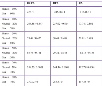
Table 1 shows the number of reliable samples and misjudge rate under different combination of human society. We can find that when the honest human is only 10% proportion of the society, many reliable samples can be obtained. However, all of them are misjudged because the misjudge rate is 1. When the honest proportion rises to 30% or 50%, the number of reliable samples will decrease, but the misjudge rate also decreases. When there are more honest humans in the society, say 90%, the number of reliable samples increases, and the misjudge rate decreases dramatically to 0.

Table 1: Number of reliable samples and misjudge rate under different human behavior

HCFA OFA RA Honest 10% Liar 90% 278 / 1 245.38 / 1 113.16 / 1 Honest 10% Neutral 20% Liar 70% 264.88 / 0.847 237.02 / 0.864 97.74 / 0.802 Honest 30% Neutral 20% Liar 50% 53.48 / 0.475 30.48 / 0.489 29.81 / 0.489 Honest 50% Neutral 20% Liar 30% 58.74 / 0.141 29.32 / 0.144 52.14 / 0.136 Honest 70% Neutral 20% Liar 10% 259.22/ 0.0001 244.34/ 0.0001 112.78/ 0.0001 Honest 90% Liar 10% 279.02 / 0 253.5 / 0 117.38 / 0

(Number of Reliable Samples /Misjudge Rate)

Simulation Results: 1) Scenario 1

In the first scenario, we evaluate the misjudge rate in our system under different confidence index threshold. The confidence index threshold ranges from

[0.2, 0.7]. Figure 4 shows the misjudge rate by three different assignment strategies we proposed. The average misjudge rate range is from [0,0.0014]. We observe that when the CI threshold is smaller, it will cause misjudge rate greater. This is because when the confidence index threshold is lower, it may produce many “reliable” samples, however, some of them may be misjudged. But if we set CI threshold to be higher than 0.7, the misjudge rate is almost zero. And we find that when CI threshold is lower than 0.5, the misjudge rate will dramatically increase. Hence we define a reliable sample and a unreliable sample is showed as below:

 A reliable sample: Confidence Index >= 0.5 & Be agreed >= 3 times.

 A unreliable sample: Confidence Index <= -0.5 & Be disagreed <= 3 times.

Figure 4: Misjudge Rate under Different Confidence Index Threshold

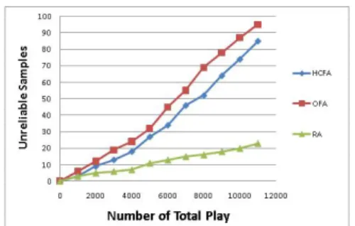
Figure 5 shows the number of reliable samples produced versus number of total play. From the results, we can see how fast the reliable samples can be produced for different strategies. Obviously we can find that in the same number of times, HCFA always has produced relatively more reliable samples. This is because the system always assigns the information with highest CI, thus, leading to a higher probability to reach CI threshold. OFA also has the same trend to let the oldest become reliable quickly. However, if the oldest takes much time to obtain higher CI or even doesn‟t get a change to reach CI threshold, it will decrease the efficiency to produce the samples. The RA strategy has the worse result due to its verification has no focus, i.e., each information takes a long time to get a change to be verified and increase CI.

On the other hand, we observe the number of unreliable samples shown in Figure 6. We can find the OFA strategies get the most chance to identify unreliable samples due to its focus on the oldest no matter positively or negatively. However, HCFA always focus the possible reliable information to be

verified first. The effiency for RA to identify unreliable samples is the worst.

Figure 5 :Reliable Samples under Different Number of Play

Figure 6 :Unreliable samples under Different Number of Play

2) Scenario 2

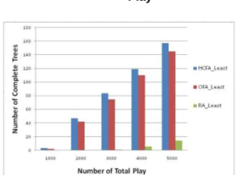
The above analysis is considering only one local scenic spot information. But in reality, players can choose to verify information previously produced in their nearby locations, and can also create a new scenic spot information. Therefore, a number of spot information will co-exist in the game system. Here, we call one spot information with many players‟ verification as a tree. So when a player want to do verification, the system should first select an appropriate tree, and then select one player‟s information from that tree for verification using the task assignment strategy. Based on the previous three task assignment, here we consider three more kinds of tree selection strategies.

 Most: Assign the tree with most reliable samples within 50 meters.

 Least: Assign the tree with least reliable samples within 50 meters.

 RA : Assign the tree with random allocate regardless of reliable samples.

We have explained before about Reliable sample (Confidence Index >=0.5 & Be agreed >= 3 times). Here, we say a tree to be a “Completed Tree”, if it has five reliable samples, implying that the mission of this tree is finished. , A completed tree is no longer assigned for verification. Therefore we may have nine

possible combinations of strategies (Three task assignment * Three tree selection ). For example, HCFA_Most means the system according to players‟ location chooses a tree which have the most reliable samples, and node‟s selection are based on HCFA task assignment algorithm. Figures 7 ~ 9 shows the results. We can find the result no matter which tree strategy (Most, Least, RA) is selected, HCFA has much more Completed Trees than OFA and RA. We also observe that in the simulated reality environment, HCFA still have better results.

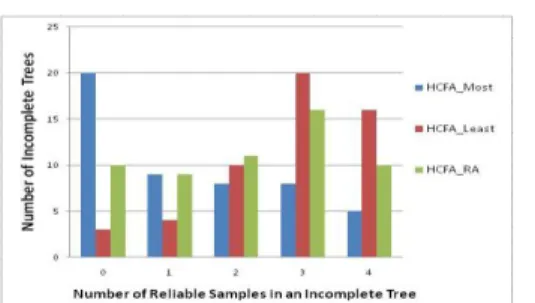
On the other hand, we further observe the number of Incomplete Tree with different number of reliable samples for HCFA_Most, HCFA_Least and HCFA_RA. We can see that even HCFA_Most produces indeed much more Complete Trees than HCFA_Least and HCFA_RA, but for the incomplete trees, HCFA_Least has more almost-complete tree (3 or 4 reliable samples in the incomplete tree) than HCFA_Most and HCFA_RA (Figure 10). So we think the HCFA_Least is more suitable than HCFA_Most.

Figure 7 : Complete Trees under Different Number of Play

Figure 8:Complete Trees under Different Number of Play

Figure 9: Complete Trees under Different Number of Play

Figure 10: Incomplete Trees with different number of reliable samples

3. "Location assisted Routing with Network Coding in Vehicular Delay Tolerant Networks”

3.1 Abstract

This paper proposed a routing protocol integrating the characteristic of flooding-based protocol and forwarding-based protocol. The main idea of our protocol is to let message would not be flooded to every node but to the nodes moving toward or moving closer to destination. When nodes contact with each other, our approach will use the path of node, node‟s moving direction and its velocity to estimate the probability to reach the destination of message. At the same time, we exploit network coding to transmit coded block instead of message fragment in order to avoid sending redundant replication, make data transmit more reliable and more robust to packet losses or delays. From the result of simulation, we could see that our protocol have a higher performance especially in the bandwidth consumption compared to other protocols.

3.2 Main Results

A.

System Model

We model a DTN as a set of mobile nodes in a vehicular environment. And there is only allowed inter-vehicle communication. Each node in the network equips GPS device. And the navigation system is

installed on every node. The nodes use the navigation system to find a shortest path to destination. The navigation system provides three kind of primitive information: trajectory, moving direction and velocity. Based on the information provided by navigation system, every node can collect navigation information contained in beacon which is broadcasted from the contact neighbors during contact time and make routing decision accordingly. The destination of message has a fixed location such as the portal to internet. A node can deliver messages to the final recipient or via intermediate nodes.

B.

Delivery Probability Estimation

We use location information to estimate the delivery probability. First of all, if there is a node that will bring the message closer to destination, we might be able to rely on it to deliver messages. So we adopt the future trajectory of node provided by navigation system as one of the estimation factors. However, the trajectory information is not enough to define good relay candidates. For example, a bus may have a fixed trajectory closer to destination but its moving direction is away from it. Therefore, the node‟s moving direction should also take into account. Finally, it is very intuitive to select a faster node to take the responsibility for delivering message. Combined the three factors, the formula we used to estimate delivery probability listed below:

Where c is the contact node, are predefined system parameters range from 0 to 1, .

Path(c) is the ratio to reach destination range from 0 to

1. Dir(c) is ratio moving toward destination range from 0 to 1. V(c) is relative velocity ratio range from 0 to 1. If the result of P(c) is greater than the predefined threshold, then the contact node c are viewed as an appropriate relay candidate.

C.

Location-assisted routing with network

Now we will give a full description of our proposed protocol. The LANC protocol executes when two nodes are within radio range and have discovered one another. It has five stages: Initialization, Probability estimation, Coding, Scheduling and Termination.

When two nodes contact with each other, they will collect metadata during initialization stage. The metadata contained in beacon includes: trajectory information of node, node‟s moving direction, velocity, rank map and purge table. The first three factors are used to estimate delivery probability as we mentioned

Input: Node A, Node C, Outgoing Buffer in A For each message M in Outgoing buffer do rank_C = rankmap_C.get(M.getID())

/*Get the rank of message by looking up the rank map */ rank_A = rankmap_A.get(M.getID())

If rank_C equals k /*message in C is full rank*/ continue

/*bypass the transmission opportunity to next message*/ End if

If C is the destination of message M f_count = min(k- rank_C, rank_A)

/*f_count is the number of forwarding coded blocks*/ Else /*C is relay node*/

power_A = estimate(A, M.getDestination()) power_C = estimate(C, M.getDestination())

f_count = min(k-rank_C, rank_A*(power_C/power_A)) End if

End for

before. The rank map is a record of independent encoding vectors of each message. In order to distinguish a coded block belongs to which message, a unique identifier will be assigned to message before encoding process at source. The rank of message is the number of independent encoding vectors. At each transmission finished, a node will check the rank of message, and records the value with corresponding message identifier. The purge table contains the identifier of message and the time it has been decoded. If the original message is decoded successfully, its identifier and the time decoding process finished will be pushed into the purge table and propagated by beacons. Nodes receive this beacon could drop coded blocks according to the same identifier to release memory space.

After obtain the metadata, the nodes will estimate the delivery probability using the formula (1) we mentioned in previous section. The procedure works as follow: for each message in buffer, if the result of P(c) is larger than threshold, then puts the message in outgoing buffer for next coding stage.

Before the transmission starting, the coding operation will code the blocks in the outgoing buffer. The RLNC is performed on the blocks with the same message identifier. In source node, a message is divided into k blocks and one or several coded blocks will be transferred with corresponding encoding vectors. The source first chooses a set of random elements from GF , then multiplies each block with the element , and adds up all the results of the multiplication together to produce a coded block. If a relay node wants to send coded blocks to another node, it operates similar operations as source does. It also chooses a set of random elements from GF , but the size of this set is the number of coded blocks with the same message identifier in its buffer. Relay node multiplies each element with encoding vector and finally adds up to produce a new encoding vector. This operation is repeated again using the same set of elements to generate a new coded block. The original message is decodable as long as the destination could receive enough linear independent encoding vectors such that the coefficient matrix formed by encoding vectors is full rank.

Before starting a transmission, we will schedule which coded blocks in outgoing buffer should be transferred first to get better performance. As we mentioned before, a message is decodable only if its encoding matrix is full rank. Therefore, the rank of message is the first factor we used to make scheduling decision. During initialization stage, a node could obtain the contact

node‟s rank map from beacon. Then the node could look up the rank map of contact node by message identifier to get the corresponding rank number. The second factor is the delivery probability to destination. We have proposed our method to estimate the probability if the contact node would reach the destination in the future. So the probability can be regarded as the power that delivering messages to the final recipient. If a node finds out that the power of its contact node is less than its power, this node would not have to transfer all the coded blocks to its contact node. Fig.1 is the pseudo code of our scheduling approach.

After the transfer, the node which received coded blocks would update the rank map, or try to recover the original message by decoding at termination stage. If a node receives a coded block, it will execute Gaussian elimination procedure to verify the incoming coded blocks is innovate to the coded blocks in buffer. If the result of checking is true, the incoming coded block will be put into buffer and increase the rank counter by one in rank map according to the identifier. After the rank map updating, if the encoding matrix of message is full rank, in other words, the number of independent encoding vector equals the size of each single encoding vector, the Gaussian elimination will be operated on it to get the inverse of encoding matrix if the node is the destination of message. The original message will be recovered by encoding the inverse of encoding matrix and coded block.

In DTNs, some nodes would continuously send the messages that have already delivered to destination

because these nodes don‟t know the messages reached their final recipient. To ease the kinds of redundant transmission and buffer occupancy, once the destination recovers the original message successfully by decoding operation, the purge table will be updated by adding the message identifier and the time it decoded. The purge table will be propagated by beacons over the network. After received the beacons, a node will purge the buffer by discarding the coded blocks with the same message identifier immediately because it is not necessary to send the coded blocks of this message anymore.

We evaluate the performance of LANC using three metrics:

 Message delivery ratio

 Average delay latency.

 Transmission overhead: The transmission overhead is defined as:

We compare LANC with another two routing protocols: Epidemic Routing and PROPHET Routing. The Epidemic Routing is a greedy approach that duplicates copies of message to every contact node. The PROPHET Routing uses history of encounter and transitivity to select a better relay node. We modified these two protocols such that they have the ability to perform RLNC.

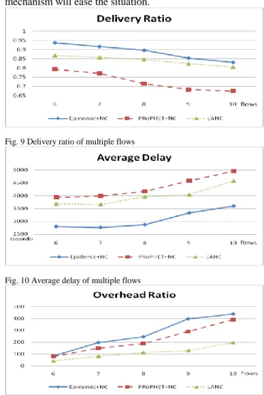
Fig.9 shows that the performance of each protocol drops down with the load of flow increase.

Once there are more flows in the network, congestion might occur at some bottleneck relay node. Our protocol uses purge table to inform other node to purge its buffer. This operation not only frees memory storage but also reduces the chance the congestion occurs. Moreover, LANC uses rank map to schedule the priority of coded blocks. If a message is already full rank, LANC will bypass the opportunity to next message.

At the same time, LANC views the results of estimation function as the probability a node would future move toward the destination, LANC could schedule coded blocks according the probability to deliver it to another node or not, so the responsibility for delivering message could be shared by a set of nodes. Even if a relay node would never reach the destination in the future, it won‟t be a problem hence the node doesn‟t have all the coded blocks.

In Fig.10, the average delay increases with the trend of flow load. The LANC has a little higher delay time than Epidemic routing with NC. The difference is about 1200 seconds. For non-real time demand such as

sending emails or uploading photos, it‟s considered acceptable. And Epidemic routing tries every possible contact opportunities, the network bandwidth it wasted must be very large. In other words, our protocol is more efficient because the bandwidth consumed by LANC is less.

As for PROPHET routing with NC, the estimation it made is based on historical encounter record, so it has a poor result. The method PROPHET routing used might be suitable for a small closed area like a concert or a lounge bar. Because LANC uses the future possible trajectory of node to predict the delivery probability, LANC could make more precise estimation in large scale outdoor environment.

Fig.11 shows that the overhead ratio of our approach is much smaller than Epidemic routing with NC and PROPHET routing with NC. The LANC will select “better” relay candidates to deliver coded block, hence our protocol require less transmissions. Although it will keep the coded blocked in buffer for a while, the purge mechanism will ease the situation.

Fig. 9 Delivery ratio of multiple flows

Fig. 10 Average delay of multiple flows

三、計畫成果自評

本計畫的主要的貢獻在設計一個定位演算法適 用於室內定位使用。而定位的精準有賴 Radio Map 的建立，因此利用人智運算,Game-with-a-purpose 的方式去設計一個 mobile Geo-tagging system， 以利有效建置此 Radio Map。

定位系統以及 mobile geo-tagging system 我 們都有實踐出實際系統，並透過實驗收集數據，確 實能達到一定的準確度以及效率。 最後，利用位置資訊，我們也開發了結合位置 以及網路編碼技術之適用於車隊的 DTN 封包轉發演 算法，實驗結果也比 related work 改善許多。 綜合以上，成就了相關 DTN routing 的基礎， 也 讓 我 們 接 續 的 研 究 能 更 有 完 整 的 面 貌 。

1

國科會補助專題研究計畫項下出席國際學術會議心得報告

日期：100 年 12 月 28 日

一、參加會議經過

本次會議在大連舉行，地點選在仲夏花園飯店，在大連靠海地方，環境優雅交通尚

稱便利。會議開始一樣從 keynote 開始，我聽了其中兩場，一場是來自日本的教授，

介紹它們的 CyberWorld 相關的大型計劃創始想法的緣起、努力與未來預期。讓我驚

嘆到日本學者做事真的非常仔細，有些實驗非常繁瑣，但是他們還是很認真地在面

對問題與思索解決方法。另一 keynote 則講得比較偏硬體方面，由於與專長興趣較

計畫編號

NSC 99－2221－E－004－005

計畫名稱

基於人智運算輔助定位分群之群組通訊在奈延遲網路的研究

出國人員

姓名

蔡子傑

服務機構

及職稱

政治大學資訊科學系

副教授

會議時間

100 年 08 月 24 日

至

100 年 08 月 26 日

會議地點

Dalian, China

會議名稱

(中文)

(英文)The 14th IEEE Internation Conference on Computational

Science and Engineering (CSE 2011)

發表論文

題目

(中文)

(英文)GWAP Design for a Mobile Geo-Tagging System With Confident

Verification

2

不相關，因此沒有特別印象。

接下來，就是我要報告論文的 session 了,我這次報告的主題是 GWAP，這是一個時坐

在手機上的實驗性質的遊戲，並帶有策略目的的遊戲，希望比較在不同策略下，可

以較有效率的產出具品質與相互驗證的結果。很榮幸有這個機會，對與會人士介紹

我們的研究，在場也有來自澳洲的學者提出問題，主持人也給了一些回響。

接著下一個 session，就是我所主持的，剛好這個 session 有來自中央資工的論文報

告，很榮幸認識了來自中央資工的周立德教授，也對他們的電子紙的應用研究留下

深刻的印象。另外，與會人士也有來自美國任教的中國教授，我們也相互留下名片，

以及交換研究心得。

二、與會心得

參加國際會議當然最重要的就是交流與吸取別人研究經驗與成果分享，雖然這個會

議舉辦在中國，參加的華人佔大多數，可是卻是有不少的外國學者與會，規模還算

不小，舉辦單位非常的用心。在晚宴時，大會主席一一唱名，每個國家都點名一位

上去發表心得，結果發現居然幾乎全世界的國度都有人參加，宴會氣氛非常熱絡，

大家都約定好下一屆再次投稿，可以繼續支持這個會議。

大會結束後最後一天，還舉辦了旅順一日遊，帶領我們參觀一些日俄戰爭時代留下

來的一些歷史景點與古蹟，參觀博物館瀋陽事變的一些文物，回憶了一些民國史實，

為這個會議畫下一個完美句點。總而言之，參加這個會議，真的得到不少面向的收

穫。

三、考察參觀活動(無是項活動者略)

無

3

四、建議

無

五、攜回資料名稱及內容

大會論文集一本

六、其他

無

GWAP Design for a Mobile Geo-Tagging System

With Confident Verification

Tzu-Chieh Tsai, Tai-Rong Yang,

Department of Computer Science National Chengchi University,

Taiwan, Taipei,

[email protected], [email protected]

Abstract—Location-based services (LBS) gain a lot of attraction recently. However, to collect necessary and accurate information to support LBS is always manpower-consuming, and may be also difficult for machine computation. “Human Computation” can therefore be adopted to attack the problems. These problems which are usually difficult for machines to solve can be easily completed by human. We can embed our purpose into a designated game. In this way, players will automatically achieve our purpose while playing the games. In this paper, we based on the concept of ‘Games with a Purpose’(GWAP) to develop a mobile geospatial tagging system. Players share their nearby scenic spot information which will then be verified by other players who come to the same place later. Thus the information collected by the system can be also reliable.

However, verification process can alter the performance of the system. We propose three different strategies on the task assignment for comparisons. Through simulation experiments, our system can indeed achieve good performance. Finally we implement the system on the smart phone (Android Phone), and do the field test to observe the results.

Keywords-Human Computation,Game with a purpose(GWAP); Mobile Geo-Tagging System; Location-Based Service.

I. INTRODUCTION

The ‘Game with a Purpose’(GWAP) genre [1,2,5] is a type of Human Computation. It is an idea that solving the problems by computers is difficult, but is easy for human. In traditional computation, a human employs a computer to solve a problem. A human provides a formalized problem description to a computer, and receives a solution to interpret. Human computation frequently reverses the roles. The computer asks a person or a large group of people to solve a problem, then collects, interprets, and integrates their solutions, by taking advantage of people’s desire to be entertained. Human computation can solve some problems that computer computation cannot currently resolve completely.

In[3],Yuen et al. gave an extensive survey of human computation systems. And the concept of GWAP which belongs to the ‘Social Game-Based Human Computation with Online-Players’, was pioneered by Luis Von Ahn and his colleagues. Especially, the ESP game, which is one kind of GWAP, was made for a variety of human computation tasks.

On the other hand, in the past few years, mobile

handheld devices have become an indispensable part of our daily lives. Integrating with some sensors (i.e., compass, camera and GPS receivers), many different new mobile applications can be developed. For example, users can know their own location via GPS on the Google Map[5], and use camera to take photographs with their location. This will allow images to be browsed on Flicker[6] or Panoramio[7], and provide large collections of publicly available geo-referenced images.

The adoption of mobile phones in recent years has brought society to the point where mobile computing technology is in the hands of the masses. Potential applications for this ubiquitous connectivity are only just beginning to be explored. One of those promising areas of investigation is the field of pervasive gaming. These experimental games are designed to examine how the emerging capabilities on offer could be practically used in the real world. Mobile social games represent a subset of this genre and utilize the interactions made between players and their relationship with the physical world.

In this paper, we integrate the concept of GWAP to develop a mobile geo-tagging system to collect reliable scenic spot information. The existing GWAP-based geo-tagging approaches focus on design, implementation and measurement of real word applications. However, they rarely focused on the performance of GWAP systems. We would design our system that will allow players to play at any urban location, including indoors, so that by-products could be generated for any desired area. The system will allow players to manually correct location on the google map. This is because GPS is usually inaccurate in the indoor environment. More importantly, players can share the scenic spot information, and other players use the information(e.g., texts, images, GPS coordinate and compass direction ) to verify to increase the confidence of the information collected.

The rest of this paper is organized as follows. Section 2 introduces related works in GWAP-based geospatial tagging systems. In Section 3, we present our analysis of such systems and compare the three proposed task assignment algorithms. In Section 4, we present the simulation results. In Section 5, we present the implementation screen on the Android phone. Section 6 concludes this paper and remarks on the future work.

II. RELATED WORKS

There are several existing GWAP-based geospatial tagging systems. [8] is an in-game agents that act as carriers for tasks and proxies to carry information from one player to another. The nature of a task is completely open-ended and predetermined by the player who created the gopher. [9] demonstrates how useful content can be generated as a by-product of an enjoyable mobile multiplayer game in which players tag geographic locations with photos or text. [10] is a location-based pervasive social game in which players use camera phones with location-based capabilities to create, share and reply to real-world missions. Most existing GWAP-based geo-tagging approaches focus on the design, implementation, and measurement of real word applications, then [11] [12] [13] focus on the performance of GWAP systems which can be improved significantly if they play with strategies.

.

III. GWAP DESIGN FOR MOBILE GEO-TAGGING SYSTEM WITH CONFIDENT VERIFICATION

A. Game Description

The players take photographs and make text description of the local scenic spot information. The shared information needs to be verified by other players to increase the reliability. We assume that each verification task must be played more than three times in order to achieve the agreed outcome of the relative majority. Also, each information will be associated with ‘confidence index’ which is increased if the other player agrees his/her provided information, and is decreased if the other player disagrees. Thus, the confidence index indicates somehow the degree of the reliability of the information. Once the confidence index of the information is greater than the predefined threshold，the information will be called as a “reliable sample”. On the other hand, we determined the information as a unreliable sample. Once the system recognizes the information as a reliable or a unreliable sample, it will no longer need to be verified again. Moreover, it is worth noting that when a player does the verification, he/she not only confirms others’ information but also has to upload photographs and text description to the server. This is to ensure players who do the verification really reach the same spot and provide good information, because the information that the verifier uploads would be also verified by the later another players.

B. Task Assignment Strategies

According to [14], we define the Confidence Index (CI) by the following equation (1).

Confidence Index = (Agree – Disagree) / T, (1) Agree is the number of verification players who consider the share information is correct. Disagree is the number of verification players who consider the share information is incorrect. T is the total number of the information that had been verified.

For system point of view, how to achieve more reliable samples in a limited number of verification is the important issue. Therefore, the assignment of the information to be verified will significantly affect the performance of the efficiency. Here, we proposed the following three verification task assignment strategies for comparisons: i. Random Assignment(RA)

The system randomly assigns a information to the player to do verification. The performance for this assignment will be used as the benchmark comparison.

ii. Oldest First Assignment(OFA)

The system assigns the oldest scenic spot information for the player to do verification until the confidence index leap over the threshold. It is noticed that using this algorithm, the information provided by the later verifier can not be verified by others. Figure 1 shows the verification flowchart for the OFA strategy.

FIGURE 1:OFA FLOW CHART

1. Player 1 shares information on local scenic spots. Then player 2 does verification and is assigned with the information of player 1 since it is the oldest. We assume player 2 agrees player 1’s share information that will make CI of player 1 to be 1. 2. According to oldest first assignment strategy, the

system will continue to assign player 1’s task to player 3 for verification. This time we assume player 3 disagrees player 1’s information that will make CI of player 1 to be 0.

3. If the CI of player 1’s information is not yet over the threshold, the system assigns player 1’s information to player 4.

4. If player 4 agrees, the CI of player 1 will become 0.33. The system continues to assign player 1’s information for next player till the CI is over the threshold we defined before, i.e. till the information of player 1 becomes reliable or unreliable sample. iii. Highest Confidence First Assignment(HCFA)

The system assigns the scenic spot information with highest confidence index for player to do verification. Figure 2 shows the verification flowchart for the HCFA strategy.

FIGURE 2:HCFA FLOW CHART

1. Player 1 shares information on local scenic spots. Then player 2 does verification and is assigned with the information of player 1 since it has the currently highest CI. We assume player 2 agrees player 1’s share information that will make CI of player 1 to be 1.

2. Therefore the system will continue to allocate player 1’s share information for player 3 to do verification. We now assume player 3 disagrees player 1’s information which will make CI of player 1 to 0. 3. Now for system, the CI’s for players 1, 2, and 3 are all

0, so system will randomly assign player’s information for next player to verify. We assume that player 2’s information is chosen for player 4 to verify. 4. If player 4 agrees, the system will continue to assign

player 2’s share information for player 5 to do verification since the CI of player 2 becomes 1 which is currently highest.

C. System Misjudgement

However, human may make mistakes or intentionally cheat while doing the verification. For example, assume that the first player shares a wrong information. In this case, we call the player is a “liar”. And unfortunately, the next player to verify is also a liar, thus, he/she will “agree” the share information provided by the first player. Therefore, in the worse case, the system may eventually judge the wrong information to be a reliable sample once it gets many liars to agree it. When this happens, a “misjudgment” is generated which produces a fake information. Figure 3 depicts the situation.

FIGURE 3: MISJUDGMENT

Now we know the system may cause “misjudgment”. To emulate the practical situation to see the effect, further we consider players’ human behaviors. We assume there are 3 kinds of characteristics for the behaviors, namely, honest, liar and neutral. “Honest” humans always do the right judgment, while “liar” humans always intentionally do the wrong

judgment. “Neutral” humans do right and wrong judgment in half. Table 1 shows the number of reliable samples and misjudge rate under different combination of human society. We can find that when the honest human is only 10% proportion of the society, many reliable samples can be obtained. However, all of them are misjudged because the misjudge rate is 1. When the honest proportion rises to 30% or 50%, the number of reliable samples will decrease, but the misjudge rate also decreases. When there are more honest humans in the society, say 90%, the number of reliable samples increases, and the misjudge rate decreases dramatically to 0.

Table 1: Number of reliable samples and misjudge rate under different human behavior

HCFA OFA RA Honest 10% Liar 90% 278 / 1 245.38 / 1 113.16 / 1 Honest 10% Neutral 20% Liar 70% 264.88 / 0.847 237.02 / 0.864 97.74 / 0.802 Honest 30% Neutral 20% Liar 50% 53.48 / 0.475 30.48 / 0.489 29.81 / 0.489 Honest 50% Neutral 20% Liar 30% 58.74 / 0.141 29.32 / 0.144 52.14 / 0.136 Honest 70% Neutral 20% Liar 10% 259.22/ 0.0001 244.34/ 0.0001 112.78/ 0.0001 Honest 90% Liar 10% 279.02 / 0 253.5 / 0 117.38 / 0

(Number of Reliable Samples /Misjudge Rate)

IV. SIMULATIOIN RESULTS

A. Simulation Setup

We analyze our mobile geo-tagging system with the following aspects: (A1) Measure the effect for different confidence index threshold, (A2) Compare the number of reliable or unreliable samples in our proposed three verification assignment. The simulation model is implemented in JAVA, with parameters shown in Table 2. The number of total play is distributed in the range of [1000, 10000], which is proportional to ascending. Each information is verified at least three times. That is, we set each node (information) must be played at least three times of agree or three times of disagree.

Table 2: Simulation Parameters.

Parameters Default Values

Number of total play 1000~10000 Number of Each node verification >=3 times (Sample threshold) Confidence Index 0.2 ~ 0.7

Previous study indicates that human behavior will cause misjudgment. Therefore, the CI threshold will be sensitive for the quality of our system performance. For simplicity,

we assume in the following simulation, the distribution for honest, neutral, and liar is 70%, 20%, and 10%, respectively.

B. Simulation Results 1) Scenario 1

In the first scenario, we evaluate the misjudge rate in our system under different confidence index threshold. The confidence index threshold ranges from [0.2, 0.7]. Figure 4 shows the misjudge rate by three different assignment strategies we proposed. The average misjudge rate range is from [0,0.0014]. We observe that when the CI threshold is smaller, it will cause misjudge rate greater. This is because when the confidence index threshold is lower, it may produce many “reliable” samples, however, some of them may be misjudged. But if we set CI threshold to be higher than 0.7, the misjudge rate is almost zero. And we find that when CI threshold is lower than 0.5, the misjudge rate will dramatically increase. Hence we define a reliable sample and a unreliable sample is showed as below:

¾ A reliable sample: Confidence Index >= 0.5 & Be agreed >= 3 times.

¾ A unreliable sample: Confidence Index <= -0.5 & Be disagreed <= 3 times.

Figure 4:Misjudge Rate under Different Confidence Index Threshold

Figure 5 shows the number of reliable samples produced versus number of total play. From the results, we can see how fast the reliable samples can be produced for different strategies. Obviously we can find that in the same number of times, HCFA always has produced relatively more reliable samples. This is because the system always assigns the information with highest CI, thus, leading to a higher probability to reach CI threshold. OFA also has the same trend to let the oldest become reliable quickly. However, if the oldest takes much time to obtain higher CI or even doesn’t get a change to reach CI threshold, it will decrease the efficiency to produce the samples. The RA strategy has the worse result due to its verification has no focus, i.e., each information takes a long time to get a change to be verified and increase CI.

On the other hand, we observe the number of unreliable samples shown in Figure 6. We can find the OFA strategies get the most chance to identify unreliable samples due to its focus on the oldest no matter positively or negatively. However, HCFA always focus the possible reliable information to be verified first. The effiency for RA to identify unreliable samples is the worst.

Figure 5 :Reliable Samples under Different Number of Play

Figure 6 :Unreliable samples under Different Number of Play 2) Scenario 2

The above analysis is considering only one local scenic spot information. But in reality, players can choose to verify information previously produced in their nearby locations, and can also create a new scenic spot information. Therefore, a number of spot information will co-exist in the game system. Here, we call one spot information with many players’ verification as a tree. So when a player want to do verification, the system should first select an appropriate tree, and then select one player’s information from that tree for verification using the task assignment strategy. Based on the previous three task assignment, here we consider three more kinds of tree selection strategies.

¾ Most: Assign the tree with most reliable samples within 50 meters.

¾ Least: Assign the tree with least reliable samples within 50 meters.

¾ RA : Assign the tree with random allocate regardless of reliable samples.

We have explained before about Reliable sample (Confidence Index >=0.5 & Be agreed >= 3 times). Here, we say a tree to be a “Completed Tree”, if it has five reliable samples, implying that the mission of this tree is finished. , A completed tree is no longer assigned for verification. Therefore we may have nine possible combinations of strategies (Three task assignment * Three tree selection ). For example, HCFA_Most means the system according to players’ location chooses a tree which have the most reliable samples, and node’s selection are based on HCFA task assignment algorithm. Figures 7 ~ 9 shows the results.

We can find the result no matter which tree strategy (Most, Least, RA) is selected, HCFA has much more Completed Trees than OFA and RA. We also observe that in the simulated reality environment, HCFA still have better results.

On the other hand, we further observe the number of Incomplete Tree with different number of reliable samples for HCFA_Most, HCFA_Least and HCFA_RA. We can see that even HCFA_Most produces indeed much more Complete Trees than HCFA_Least and HCFA_RA, but for the incomplete trees, HCFA_Least has more almost-complete tree (3 or 4 reliable samples in the inalmost-complete tree) than HCFA_Most and HCFA_RA (Figure 10). So we think the HCFA_Least is more suitable than HCFA_Most.

Figure 7 : Complete Trees under Different Number of Play

Figure 8:Complete Trees under Different Number of Play

Figure 9: Complete Trees under Different Number of Play

Figure 10: Incomplete Trees with different number of reliable samples

V. SYSTEM IMPLEMENTATION

We performed our experiment in NCCU Campus. There are 24 Players for this experiment. Each player take a Android phone to proceed. Table 3 describes the experimental environment and resource we set.

Table 3: Experimental Setup

Environment NCCU Campus

Android Phone HTC Hero & HTC Desire

Version Android 2.1

O.S. Microsoft Windows XP

System Language Java

Sensors GPS , Camera , Compass

Figure 11: System Architecture

Figure 11 depicts our mobile system architecture. System adopts client-server architecture. The server is responsible for data storage and task assignment, while the clients are mobile players and connected to the server via the Internet. There are two game-playing rules: Sharer and Verifier, and players are allowed to switch between the roles during run time.

A. Experimental Setup

When a player starts our application in Android phone, it meanwhile will open the GPS sensor. Figure 12 shows the login page. We combine the Google account as part of our entrance. This has the advantage that we do not have to maintain the players’ account and password, and players also can be more relieved to use our system. GPS may be not available due to indoor environment, so Figure 13 shows the manual correction screen, i.e. the player can self decide its location. If the player corrects the location dishonestly, its share information will be disagreed by other players according to our verification design. Figure 14 shows the main screen in NCCU campus. We use landmark at each NCCU building, according to the player’s location. Then the system will show the building name (for example, Daren Building Nearby). Here we also integrate the compass sensor, and thus user can see self direction and can play share or verify. If the user choose share, Figure 15 shows the share screen; player enters the text and photo information to the server.

Figure 12: Login Screen Figure 13: Confirm location Screen

Figure 14: Main Screen Figure 15: Share Screen

Figure 16 depicts we combine the compass and the Google map rotate view on the camera screen. When the player clicks verify button, the system will assign the task for the player. (Task assignment strategy had been explained in Section III). Figure 17 depicts the assigned screen. The player may not like to solve the task, so we apply change button for the player to switch task.

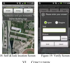
In Figure 18, when the player accepts this task, the player can see the self and scenic spot direction. And then according to text description and photograph, the player judges whether the share information is true (Agree) or false (Disagree). The player also can see self and task location to find the object easily. Figure 19 depicts the verify screen, the difference from the share mode is that we add the agree and disagree button.

Figure 16: Camera Screen Figure 17: Task assigned Screen

Figure 18: Self &Task location Screen Figure 19: Verify Screen

VI. CONCLUSION

In this paper, we propose three task assignment strategies for our mobile GWAP-based geo-tagging system. In our system, everyone could be a sharer to share local scenic spot information or switch to be a verifier to exam local task is true or false. By using the concept of game with a purpose, our main purpose is that collect the production of usable by-products through mobile game-play and these by-product are reliable and easy identification..

We analyze our system in different confidence index threshold to achieve the best performance. Also, in the real environment, we further have nine possible combination of strategies. The simulation results show that HCFA_Least is most suitable in our system. We implement our mobile geo-tagging system in Android phone and choose 24 players for experiment it in the real world.

In the future, the social network element can be added to our system. This will let the system be more interesting, and can attract more people to play with our system.

REFERENCES

[1] L. von Ahn. Games with a Purpose. IEEE Computer, 39(6):92–94, June 2006.

[2] L. von Ahn, and L. Dabbish. Designing games with a purpose. Communications of the ACM, 51(8):58–67, August 2008.

[3] M.-C. Yuen, L.-J. Chen, and I. King. A survey of human computation systems. In the 2009 International Conference on Computational Science and Engineering, 2009.

[4] E. Law and L. von Ahn. Input-agreement: A new mechanism for data collection using human computation games. In ACM CHI, 2009. [5] GWAP: http://www.gwap.com/gwap/

[6] Google Maps. http://maps.google.com/

[7] GeoTagging Flicker. http://www.flickr.com/groups/geotagging/

[8] S. Casey, B. Kirman, and D. Rowland. The gopher game: a social, mobile, locative game with user generated content and peer review. In International Conference on Advances in Computer Entertainment Technology, pages 9–16, 2007.

[9] M. Bell, S. Reeves, B. Brown, S. Sherwood, D. MacMillan, J. Ferguson, and M. Chalmers. Eyespy: Supporting navigation through play. In ACM SIGCHI, 2009.

[10] L. Grant, H. Daanen, S. Benford, A. Hampshire, A. Drozd, and C. Greenhalgh. MobiMissions: the game of missions for mobile phones. In ACM SIGGRAPH, 2007.

[11] Ling-Jyh Chen, Yu-Song Syu, Bo-Chun Wang, and Wang-Chien Lee. An Analytical Study of GWAP-based Geospatial Tagging Systems. IEEE International Conference on Collaborative Computing: Networking, Applications and Worksharing (CollaborateCom'09), Washington D.C., USA, 2009.

[12] Ling-Jyh Chen, Bo-Chun Wang, and Kuan-Ta Chen. The Design of Puzzle Selection Strategies for GWAP Systems. Journal of

Concurrency and Computation: Practice and Experience, John Wiley & Sons Ltd., volume 22, number 7, pp. 890-908, May, 2010.

[13] Ling-Jyh Chen, Bo-Chun Wang, and Wen-Yuan Zhu. The Design of Puzzle Selection Strategies for ESP-like GWAP Systems. IEEE Transactions on Computational Intelligence and AI in Games, volume 2, number 2, pp. 120-130, June, 2010.

[14] Shun-Ching Huang.A Study on Taiwan’s Consumer Confidence Index and Private Consumption Expenditure